Three-Dimensional Tomography of Coseismic Ionospheric Disturbances Following the 2018 Palu Earthquake and Tsunami from GNSS Measurements

Preliminary research analyzed the Coseismic Ionospheric Disturbances (CIDs) of the strike-slip earthquake that occurred in Palu on September 28, 2018 (Mw = 7.5) and the materialization of a TEC anomaly with an amplitude of 0.4 TECU approximately 10–15 min later. The TEC anomaly amplitude is also affected by the magnitude of the earthquake moment; therefore, 3D analysis is needed to determine the spatial distribution of the ionospheric disturbances. This research aims to analyze the ionospheric disturbance of an earthquake in 3D using the Global Navigation Satellite System (GNSS) from the Geospatial Information Agency (BIG) or InaCORS stations spread over Sulawesi, Kalimantan, West Nusa Tenggara, East Nusa Tenggara, Bali, and Java with a 30 s sampling interval using GLONASS and GPS satellites. The checkerboard accuracy test was also carried out to evaluate the reliability of the 3D tomography model. The result showed that CIDs occur to the north and south of the epicenter around the equator, following the N-S Asymmetry theory. Furthermore, the tomography results indicate the presence of dominant and positive anomaly values at an altitude of 300–500 km. This follows the characteristics of variations in the ionosphere layer, where an altitude of 300–500 km is included in the F layer. The dominant anomaly at an altitude of 300 km is in accordance with the theory of the ionosphere’s height, which experiences maximum ionization at an altitude of ∼300 km (F layer) by Chapman’s profile. We also conducted preseismic studies of ionospheric anomalies before the earthquake as an additional analysis.

Introduction

GNSS is used to estimate the ionospheric total electron content (TEC) by integrating several electron densities along the line of sight (LoS) between the receiver and the satellite (Cahyadi and Heki 2013; Jin and Su, 2020). The TEC value has been measured by various types of ionospheric disturbances caused by several phenomena, such as mine blasts (Calais et al., 1998), volcanic eruptions (Heki, 2006; Nakashima et al., 2016; Cahyadi et al., 2020), and launches of ballistic missiles (Ozeki and Heki, 2010). Research of the ionospheric electron density variation influenced by earthquakes has been conducted, and some coseismic ionospheric disturbances have been observed, which provided insights into earthquakes (Calais et al., 1998; Ozeki and Heki, 2010; Tsugawa et al., 2011; Cahyadi and Heki, 2013, 2015; Jin et al., 2014; Shah and Jin, 2015; Shah et al., 2020; Cahyadi et al., 2021, 2022).

In recent years, CID has been investigated using global navigation satellite systems (GNSS), including the global positioning system (GPS), with techniques such as GPS occultation (Okazaki and Heki, 2012) and the ground-based GNSS-total electron content (TEC) method (Cahyadi and Heki 2013, 2015). TEC corresponds to the number of electrons integrated along the line of sight (LoS) of GNSS microwave signals between satellite and ground receivers. Some CID research on the occurrences of earthquakes in Sumatra has been reported for the 2004 Sumatra-Andaman 9.1 Mw (Heki, 2006; Choosakul et al., 2009; Astafyeva et al., 2014), 2005 Nias 8.6 Mw (Hasbi et al., 2009; Cahyadi and Heki 2013), 2007 Bengkulu 8.5 Mw (Cahyadi and Heki 2013), and 2012 North Sumatra with an 8.6 Mw mainshock and 8.2 Mw aftershock (Cahyadi and Heki 2015). The strike-slip earthquakes detected in Sumatra and the 2012 South Sumatra Earthquake with 7.9 Mw, 8.6 Mw, and 8.2 Mw, respectively. Cahyadi et al. (2018) research on the CID of the 2016 West Sumatra Earthquake mainly focused on the analysis of time occurrence and the magnitude of the CID anomaly at the receiving station’s location.

Research on the 2018 Palu earthquake was previously conducted by Marchetti et al. (2020), which focused on analyzing pre-earthquake anomalies using Swarm and China Seismo-Electromagnetic Satellite (CSES). The research related to the anomalies investigation before the earthquake was also carried out by De Santis et al. (2020) using ionosonde data and Swarm satellites. The electron density observed using the ionosonde and Swarm satellites increased significantly 33 days before the earthquake. The anomaly was commonly detected using Swarm satellites and ionosondes. However, both studies did not analyze GNSS-TEC data to observe ionospheric anomalies before the earthquake. Pre-earthquake anomaly research using GNSS-TEC data was conducted by He and Heki (2016), who studied the three-dimensional spatial structure of the ionosphere’s total electron content (TEC) anomaly before the three recent major earthquakes in Chile, South America, namely the 2010 Maule earthquake (Mw 8.8), Iquique 2014 (Mw 8.2), and Illapel 2015 (Mw 8.3). He and Heki (2018) also conducted three-dimensional tomography of ionospheric electron density anomalies immediately before the 2015 Illapel Mw8.3 earthquake in Central Chile. The modeling results were in the form of a 3D model of the ionospheric disturbance at 25 min, 5 min, and 1 min before the earthquake occurred. The reconstructed anomalies are positive and negative regions distributed along the geomagnetic field lines at altitudes of ∼200 and ∼400 km. Previous studies only analyzed the ionospheric disturbance before the earthquake. Therefore, 3D tomographic modeling is required after the occurrence. It also showed that the earthquake mechanism analyzed has a thrust-fault focal mechanism. However, this present research aims to analyze earthquakes with varying focal mechanisms from He and Heki (2018), such as those with a strike-slip, namely the 2018 Palu Earthquake.

On September 28, 2018, an earthquake occurred in Palu, Sulawesi Island, Indonesia at 10:02:44 UT at 0.18° S, 119.84° E with a magnitude of Mw 7.5. The earthquake occurred as a strike-slip fault at shallow depths in the Molucca Sea microplate, part of the Sunda tectonic plate. The September 28, 2018 earthquake was preceded by a series of small to moderate earthquakes in the hours before and after the mainshock and generated a tsunami (USGS, 2020). The Indonesian Agency for Meteorology, Climatology, and Geophysics (Badan Meteorologi, Klimatologi dan Geofsika—BMKG) issued a tsunami warning for a local tsunami within minutes of the earthquake (BMKG, 2020).

Cahyadi et al. (2022) recently analyzed the CID of two earthquake cases in Indonesia, namely that of 2016 West Sumatra and 2018 Palu. The CID of the 2018 Palu Earthquake occurred ∼13 min later, followed by a tsunami 20–25 min later. However, it only analyzed disturbances in the ionosphere in 2D at an altitude of 300 km. To better investigate the phenomenon, a 3D modeling process can be employed to determine the distribution and direction of movement of ionospheric disturbances at each height of the ionospheric layer. Therefore, this paper aims to continue the research of Cahyadi et al. (2022) by analyzing the ionospheric disturbance in 3D at each ionospheric height using the 3D tomography method. This also analyzed the CID of earthquakes and electron density anomalies using InaCORS (Indonesia Continuously Operating Reference Station) and GNSS-TEC data. As an additional analysis, we also conducted a study related to preseismic anomalies from 40 days before the earthquake as an additional analysis.

Materials and Methods

STEC From GNSS Data

The GNSS stations used in this research were from the Geospatial Information Agency (BIG), or InaCORS, spread over Sulawesi, Kalimantan, West Nusa Tenggara, East Nusa Tenggara, Bali, and Java with 30 s sampling intervals including GLONASS and GPS satellites. A total of 16, 10, 10, 1, and 56 InaCORS stations are located in Sulawesi, Kalimantan, East Nusa Tenggara, West Nusa Tenggara, and Java with average distances of ∼96, ∼185, ∼87, ∼87 and ∼44 km, respectively. In total, 93 GNSS stations were used to examine the anomalies of the 2018 Palu Earthquake, as shown in Figure 1A. The condition of one-direction geometry between the epicenter and GPS receivers is shown in Figure 1B. This condition is important because it enables shallow LOS penetration with the CID wavefront.

FIGURE 1

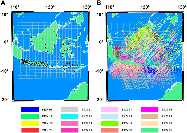
FIGURE 1. (A) The distributions of GNSS stations from InaCORS (black triangle) used in the 2018 Palu Earthquake. The yellow star marks the epicenter of the 2018 Palu earthquake with a magnitude of 7.5 Mw that occurred at 10:02:44 UT. (B) The distribution of LoS over the area blocks tomography with different colored lines used to represent each on the satellite.

A Slant TEC (STEC) value was obtained from the GNSS phase difference data conversion process between L1 (∼1.5 GHz) and L2 (∼1.2 GHz) using an ionospheric linear combination as follows:

$∆STEC=\frac{1}{40.308}\times \frac{f_1^2{f}_2^2}{\left(f_1^2{-f}_2^2\right)}\times \left({\rho }_1-{\rho }_2\right),$

where f₁ and f₂ are the carrier phase frequency, ${\mathit{\rho }}_{\mathit{1}}$ and ${\mathit{\rho }}_{\mathit{2}}$ represent the carrier phases from f₁ and f₂, respectively, and the phase difference (${\mathit{\rho }}_{\mathit{1}}-{\mathit{\rho }}_{\mathit{2}}$) is expressed with the unit of meters (Heki, 2021). This research is focused on GPS satellites 21 and 25 due to the CID’s consistent appearance, as illustrated in Figure 2A. These GPS satellites are used, and both are visible from the studied region immediately before the mainshock (10:03 UT). However, in the reconstruction of tomographic 3D modeling, satellite GPS numbers 21, 25, and all the satellites in Figure 2B will be used.

FIGURE 2

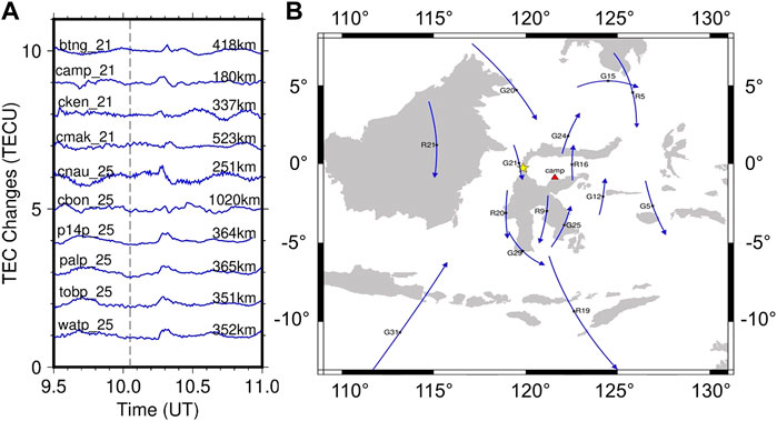
FIGURE 2. (A) Time series changes in TEC for the 2018 Palu Earthquake at 9.5–11 UT by GPS atellite 21 and 25. (B) Trajectories of SIP during the 2018 Palu Earthquake and a large yellow star indicate the epicenter’s location.

The LoS will have an intersection point with the ionosphere when the GNSS satellites transmit microwave signals in both L1 and L2 frequencies. This intersection is called an ionospheric pierce point (IPP) at an altitude of ∼300 km, and its projection onto the earth’s surface is named a sub-ionospheric point (SIP). The SIP position is calculated using the formula developed by Klobuchar (1987). This research was conducted using satellites with no threshold or null elevation angles, as indicated by the SIP position, far from the zenith station.

After determining the STEC anomaly value, it is distributed to the cube block passed by the beam (LoS) by considering its individual length. The checkerboard test model area is made the same as the LoS distribution area, as shown in Figure 1. The trajectory plotting result of GPS and GLONASS satellites in the 2018 Palu Earthquake was found at 9,5—10,5 UT, as shown in Figure 2B. The GPS satellites which orbit during an earthquake are numbers 5, 12, 15, 20, 21, 24, 25, 29, and 31, while GLONASS are numbers 5, 9, 16, 19, 20, and 21.

The one-direction geometric condition between the epicenter and the GPS receiver was not found in this case. CIDs appeared after the mainshock and were detected by GPS satellites 21 and 25 with maximum amplitudes of 0.4 TECU (Cahyadi et al., 2022). This led to changes in STEC modeled using the reference curves obtained by fitting cubic polynomials of time to the vertical TEC (VTEC) (Ozeki and Heki 2010).

Set-Up of Voxels for 3D Tomography

The input data for the calculation of the tomographic 3D block electron density anomaly are the derivative of the residual TEC (STEC) slant. The 3D blocks of ionospheric electron density were set up with the dimensions of 1 ° × 1 ° × 75 km over the Sulawesi, Kalimantan, Java, and surrounding areas, as shown in Figure 1A. The value of the STEC calculation results was distributed to the cube blocks passed through LoS by considering the length of each cube block with homogenous electron density. LoS penetrates multiple blocks, and the STEC residual can be expressed as the sum of the products of the penetration lengths and electron density anomalies of individual blocks, as shown in Figure 3.

FIGURE 3

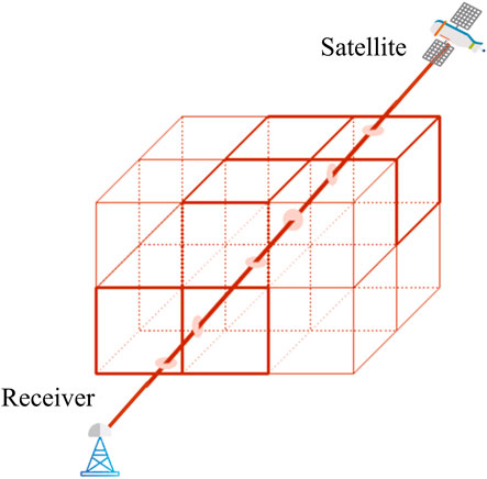
FIGURE 3. Scheme of the ionosphere divided into voxels. The basic function (δ) equals 1 for the darker cubes (i.e., those “illuminated” by the ray) and 0 otherwise.

In this case, the ionosphere is divided into voxel, therefore, the basic function is defined as follows:

$\delta \left(\lambda ,\varnothing ,h\right)=\{\begin{array}{c}1ifthecellilluminatedbytheray\\ 0otherwise\end{array}(1)$

The penetration length is the distance between the two intersections of LoS with the block surface using simple geometric calculations in Eq. 2 from Fernandez (2004). Since the research area spans only a few degrees in latitude, the Earth is considered a sphere (its fattening is neglected) with an average radius. Figure 1B shows the geometry of LoS penetrating the blocks at an altitude of 300 km.

$∆{STEC}_i={\sum }_{j=\mathit{1}}^n{A}_{ij}{x}_j+e_i(2)$

The set of equation 2 for all LoS is written in a matrix form as

$y=AX+E(3)$

where y is a vector composed of STEC anomaly ($∆{STEC}_i$), $A$ is a jacobian matrix composed of $A_{ji}$, $X$ is a vector composed of unknown parameters in the form of STEC anomaly in each block ($x$), and $E$ is an error. Value of $X$ can be estimated using the following equation:

$X={\left(A^{T}A\right)}^{-1}{A}^{T}y(4)$

Although LoS is densely distributed, they do not penetrate all the blocks, specifically above the oceanic areas. This implies a certain constraint needs to be introduced to regularize the least-squares inversion. In this situation, a continuity constraint was applied, assuming that neighboring blocks have the same electron density anomalies with a specific allowance for the difference; and also use constraints around zero (Chapman function) to calculate neighbor voxel values based on altitude. By using this method, the voxel calculation value will be more realistic, following the observations by Muafiry and Heki (2020). One block normally consists of six neighboring blocks, namely up, down, north, south, east, and south, and all these pairs were added to the normal matrix as virtual observations (Nakagawa and Oyanagi, 1982). The non-juxtaposed lock pairs were not constrained because the tolerance corresponds to the virtual data’s “observation” error and the standard deviation of the actual differences between the adjacent blocks. It is assumed that the tolerance was 0.10 in 10¹¹ electrons/m³, equivalent to 1 TECU, or 10¹⁶ electrons/m², for a penetration length of 100 km. The influence of this value on the tomography results will be discussed in the next section. Coster et al. (2013) stated that the STEC observation error was also assumed to be 0.2 TECU, a few times as large as the typical error for differential GNSS VTEC measurements, which is consistent with the post-fit STEC residuals. The resolution of 3D tomography and its accuracy will be further discussed in this research.

Result

Resolution Test

A standard way to investigate the reliability of the 3D tomography solution is through the checkerboard resolution test. While conducting the checkerboard test, the real satellite/station geometry was kept while the STEC data were synthesized. The electron density anomalies were assumed at ±0.50×10¹¹ electrons/m³, as shown in Figure 4-upper panel.

FIGURE 4

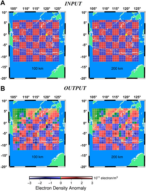
FIGURE 4. (A) The 3D pattern of electron density anomalies for the checkerboard resolution test. (B) Results of the checkerboard resolution test of the pattern.

Figure 4 (bottom panel) shows the distribution of the anomalies recovered using the synthetic data, suggesting that the spatial structures can be well resolved, with the recovered amplitudes accounting for about two-thirds of the input. Therefore, by comparing the two map views at different altitudes, the resolution at higher altitudes (200 km) was slightly worse than that at lower heights (100 km). This reflects better coverage and more penetration of LoS for lower blocks, as shown in Supplementary Figure S1 for altitude 100 km to 400 km. The figure also suggests that the resolution is higher and poorer above the land area and the ocean, respectively. The checkerboard test generally shows the high performance of the researched 3D tomography in the region of interest. Figure 4 shows that the resolution test results are poor at the left top of the bottom panel because the number of LoS distributions is scarce in that area. This is because only a few stations are used in the area, and the observed satellite objects are only GPS and GLONASS.

A second resolution test was also conducted to strengthen the tomographic modeling results by recovering a pattern consisting of a pair of positive and negative anomalies (0.6 × 10¹¹ el/m³) at low and high altitudes, respectively, on a neutral background (Figures 5A,C, as an input). The result, shown in Figures 5B,D, as an output reproduces properly, the assumed pattern of the positive anomaly is reduced to ∼2/3 the amplitude of the input model due to constraints at altitude of 300 and 400 km. Similarly, positive and negative anomalies in the latitude profile recovered properly, with only weak smears in the surrounding blocks not exceeding a few percent of the assumed anomalies.

FIGURE 5

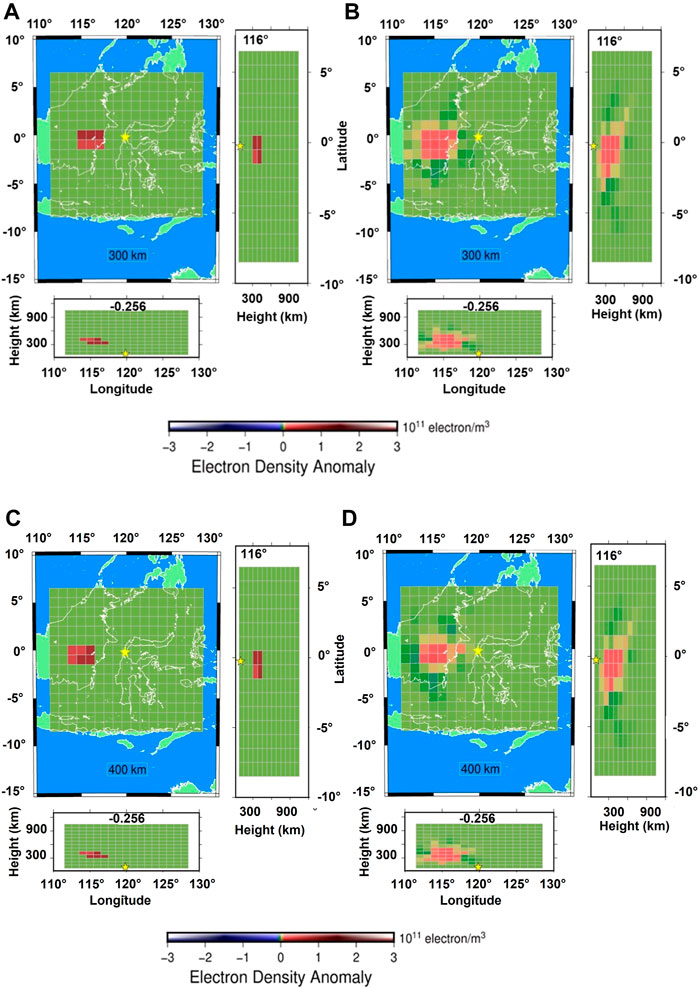
FIGURE 5. Second resolution test for a pair of positive and negative anomalies. The left and right panels are horizontal views and latitudinal profiles of the assumed pattern anomalies (A,C) and the output from the 3D tomography (B,D). On the right panel is shown a cross-section of the main profile along the longitude of 116°E. Meanwhile, the lower panel is a cross-section of the main profile along the latitude of 0.256^oS. So, the right and lower panels describes the profile in the dimensions of a given longitude and latitude, respectively. The 3D tomographic model with latitude and longitude profile formation is also used by Muafiry and Heki (2020) in describing the sporadic conditions in Japan.

Tomography Results

The results of the 3D tomography modeling are presented in the time range from when the earthquake occurred (10.03 UT) until 10.20 UT in Figures 6(A-R). In Figures 6(A-F), the ionosphere is in a normal state, as indicated by the model’s color, without an anomaly in the ionosphere. At 10.09 UT (Figure 6G), CID began to appear to the south of the epicenter, marked by a positive red anomaly value until 10.16 Figure 6(n). The range of occurrence of ionospheric disturbances is indeed a curt phenomenon (only a few minutes) shown in Figures 6(G-O). This description is in accordance with the Cahyadi et al. (2022) study, which showed CID occurred ∼13 min after the mainshock. At 10.18 UT, the ionosphere has 226 started to return to normal as shown in Figures 6(P-R).

FIGURE 6

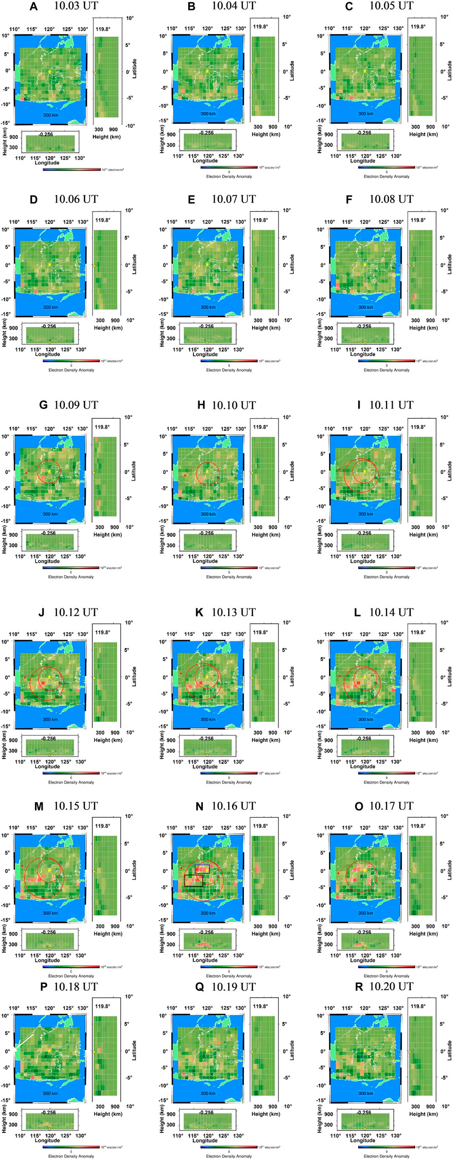
FIGURE 6. (continued).

During CID, 13 min after the earthquake (10.16 UT), positive anomaly values were found at an altitude of 300–500 km near the epicenter, as shown in Figure 7. This is in accordance with the characteristics of variations in the ionosphere layer, where an altitude of 300–500 km is included in the F layer, which has the largest ionization and electron density compared to other altitudes. Fernandez (2004) stated that the electron density is mainly concentrated at a maximum between 200 and 500 km, following the Chapman profile. The CID shown by the tomography model matches the SIP position of the GPS satellites 21 and 25, which have succeeded in observing the TEC anomaly. We also estimated the vertical profile of electron density using the IRI model (https://irimodel.org/) on September 28, 2018 and the time when the CID occurred at 10.16 UT. The modeling results show that the highest electron density is located at an altitude of 320.4 km, as shown in Supplementary Figure S2. This supports 3D tomographic modeling, which is modeled at the height of the 3rd ionospheric layer with an altitude of ∼300 km (Chapman, 1931).

FIGURE 7

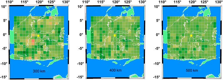
FIGURE 7. Tomography results of the 2018 Palu Earthquake at 10.16 UT in difference altitude.

Another anomaly detected by the 3D tomographic model shown in Figure 6(n) (black box) could be caused by acoustic waves generated by several earthquakes that occurred before the mainshock (Mw7.5 at 10.16 UT). The USGS (https://earthquake.usgs.gov/earthquakes/) recorded several fairly large earthquakes occurring in the 3 h to 5 min before the main earthquake. The location of the epicenters of these earthquakes can be seen in the figure (Supplementary Figure S3). Meanwhile, the ionospheric anomaly in the 3D tomography Figure 6(n) (blue box) is likely caused by the acoustic wave of the main earthquake.

We performed a statistical test using residual values from the results of 3D tomography modelling. The test was carried out by comparing the distribution results of the post-fit STEC in five epochs, as shown in Figure 8. The post-fit residual showed much smaller dispersion, and its standard deviation is similar to the assumed STEC observation errors (0.2 TECU). The results before and after modeling showed a decrease in the standard deviation value. This decrease in value indicates that the results of the 3D tomographic disturbance of the ionosphere have been well modeled.

FIGURE 8

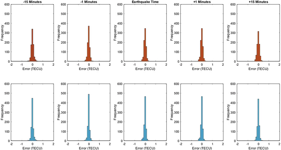
FIGURE 8. Distribution of STEC anomaly input (orange) and post-fit residue (blue).

Discussion

The 3D tomography model for the 2018 Palu Earthquake was investigated in 8 altitude layers (100–800 km), as shown in Figures 6, 7. The CID occurred ∼13 min after the mainshock. The results of tomographic processing were processed and visualized at the mainshock and when the CID was detected at intervals of every minute as shown in Supplementary Figure S4. However, 13 min after its occurrence (10.16 UT), there was an increase in electron density, which corresponds to the propagation speed of acoustic waves at an altitude of 300 km. In this study, we use the least square method to obtain the value of wave velocity that disturbs the ionosphere. The wave velocity in this research refers to Cahyadi et al. (2022) with the speed measured using GPS satellites 21 and 25 of 0.97 ± 0.191 km/s and 1.08 ± 0.039 km/s which indicates acoustic waves (Nakashima et al., 2016). Liu et al. (2020) found the speed was close to 0.3 km/s, which is a gravity wave in the 2018 Palu Earthquake, but unfortunately in this study we did not find any gravity waves. Sound velocity scales with the square root of the temperature, and the increase in velocity with altitude bends the ascending acoustic waves downward. A minimum velocity at a height of ∼100 km, caused by the temperature inversion, traps waves and lets them propagate horizontally, which is too low to disturb the ionosphere (Heki and Ping, 2005).

The value of ionospheric disturbance obtained in this study is minimal, with a maximum amplitude of 0.4 TECU. The value that is not too large is in accordance with research conducted by Cahyadi and Heki (2015), which states that earthquakes are generally not strong enough to cause disturbed electron density. The positive anomaly values were found in the 300–500 km altitude layer, where the dominant anomaly was at an altitude of 300 km. This is in accordance with the characteristics of variations in the ionosphere layer, where an altitude of ∼300 km is included in the F layer, which has the largest ionization and electron density compared to others. The CID shown by the tomographic model corresponds to the SIP position of the GPS satellites 21 and 25, which have been successful in observing the TEC anomaly. Figure 9 shows a tomographic model for each altitude (300–500 km) and the observing satellite’s SIP position (black circle).

FIGURE 9

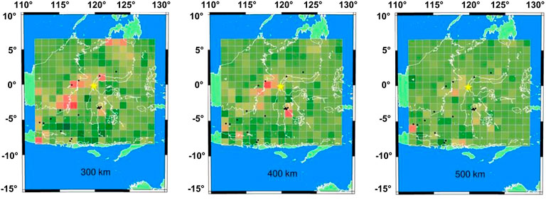
FIGURE 9. Distribution of TEC and SIP anomalies on 3D tomographic models of the 2018. Palu Earthquake at 10.16 UT (∼13 minutes after the earthquake). Black circle is the SIP where CIDs occur that are detected from GPS satellites 21 and 25.

Figure 9 aims to validate the location of the positive anomaly with the SIP position of the satellites observing the CID, namely GPS satellites 21 and 25. There is a positive anomaly (red voxel) located following the SIP position. However, red voxels do not match the SIP position as in 125^oE; 6^oN (Figure 9A). This is due to the use of the continuity constraint described in sub-chapter 2.2. While the SIP position as in 118^oE follows the green voxel; -4^oN (Figure 9A). Even though the voxel is not a block area that contains a positive anomaly, this is because the satellite detects a small anomaly value (STEC) so that the detected anomaly is not red (strong negative anomaly).

The tomography results at 10.12 UT (Supplementary Figure S4) show modeling ∼10 min after the earthquake and depict an increase in the time series (CID value). It also visualizes anomalies in the range of 10.13 UT to 10.20 UT because GNSS data were used for its analysis every minute. Conversely, the tsunami in the 2018 Palu Earthquake occurred at 10:23, which is 20–35 min later. However, by observing the CID that occurred about 13 min later, an early warning system based on observations was applied regarding the possible occurrence of a tsunami after the mainshock (BMKG, 2020).

The CID directivity of the 2018 Palu Earthquake is generally to the southwest as shown in Figure 6, according to the directivity by Heki and Ping (2005). However, there is still a diffuse motion caused by an earthquake with Mw > 5 following it, as shown in Figure 10. The series of earthquakes that occurred in Palu started with foreshocks of Mw 6.1 at 07.03 UT and Mw 5.2 at 08:25 UT. Also, this was followed by aftershocks in the next few hours, Mw 5.8 at 10.25 UT and Mw 5.0 at 21.24 UT. In addition, Figure 9 at the Mw 7.5 point shows focal mechanism solutions for the earthquake that indicate rupture occurred on either a left-lateral north-south striking fault, or along a right-lateral east-west striking fault.

FIGURE 10

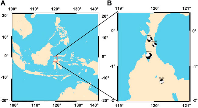
FIGURE 10. (A) Location index (window). (B) Earthquake focal mechanisms of the 28 September 2018 Palu Earthquake. Moment tensor values were obtained from the Global CMT Catalog website.

Precursor Anomaly

Marchetti et al. (2020) analyzed the presumed precursors that appeared before the 2018 Palu earthquake using the Swarm and CSES satellites, which observed changes in the ionosphere before the earthquake. These observations suggests an increase in electron density at night. We analyzed ionospheric disturbances for 40 days before the earthquake using GNSS-VTEC data to check whether there was a long-term preceismic anomaly. From the processing results, we follow the definition of ionospheric disturbance according to the observations made by Borries et al. (2015) in Equation (5), which compares the deviation value with the median value in the form of a percentage. The deviation value is obtained from the difference between the average TEC value and the median TEC value. The average TEC value with the median TEC can be seen in the table in the Supplementary Table S1.

$∆VTEC=\frac{VTE{C}_{average}-VTE{C}_{med}}{VTE{C}_{med}}\times 100\%.(5)$

From the processing results, we analyze the magnitude of the deviation that occurs in the time series as in Supplementary Figure S5. It can be said to be an anomaly if the deviation >±30% (Danilov, 2022). The deviation was found at DOY 231—234 which is Dst Index value was checked from https://wdc.kugi.kyoto-u.ac.jp/dst_provisional/. The absolute value of the Dst Index shows relatively low values < 50 nT, which means that the geomagnetic activity is relatively calm, and the resulting anomaly is likely a precursor.

There is a slight difference between the results of processing anomalies before the earthquake in this study and Marchetti et al. (2020). In the 40 days before the earthquake, the electron density observed by the Swarm and CSES satellite anomaly occurred, which was marked by a positive anomaly, while the observation method using GNSS-TEC contained negative anomalies in the same range. This difference occurs due to changes in the electron density profile of the ionosphere layer from the use of different data. Muafiry and Heki (2020) observed a short-term anomaly indicated by a nearly balanced positive and negative anomaly, indicating that the anomaly was created by electron transport in different ionospheric layers.

Conclusion

This research analyzed the 3D tomography of the ionospheric electron density anomalies of the 2018 Palu Earthquake (Mw7.5) using GNSS-TEC data observed by InaCORS spread in Sulawesi, Kalimantan, West Nusa Tenggara, East Nusa Tenggara, Bali, and Java. The CID anomaly was observed 10–15 min after its occurrence with an amplitude of 0.4 TECU. Based on the 3D tomography modeling results, we observed changes in the ionosphere layer during an earthquake until CID occurred (10.03 UT—10.20 UT). At the time of CID, i.e., ∼13 min after the earthquake (10.16 UT), the southern region of the epicenter experienced an increase in the number of electrons indicated by a positive anomaly.

The 3D model results of the 2018 Palu Earthquake are shown at an altitude of 100–800 km. The tomography results indicate the dominant anomaly value at an altitude of 300 km. This is explainable by Chapman’s Model, which experiences maximum ionization at an altitude of ∼300 km (F layer). The data shows noise near the epicenter caused by foreshocks and aftershocks a few hours before and after the mainshock. To test the reliability of the performed tomographic 3D model, we used the checkerboard test. The accuracy test results show that the lower altitude of 100 km gives better results than 200 km. This is because the area with lots/full LoS gives good accuracy test results.

Data Availability Statement

The original contributions presented in the study are included in the article/Supplementary Material; further inquiries can be directed to the corresponding author.

Author Contributions

Conceptualization: MC and IM; methodology: RR, BM, and MW; software: MP; validation: MC and BM; formal analysis: MC and RR; investigation: DA and MW; writing—original draft preparation: MC and MW; writing—review and editing: IM, B.M, and MP; visualization: DA; supervision: MC and IM; and funding acquisition: DA and BM. All authors have read and agreed to the published version of the manuscript.

Funding

This research was funded by the project scheme of the Publication Writing-IPR Incentive Program (PPHKI) 2022.

Conflict of Interest

The authors declare that the research was conducted in the absence of any commercial or financial relationships that could be construed as a potential conflict of interest.

Publisher’s Note

All claims expressed in this article are solely those of the authors and do not necessarily represent those of their affiliated organizations, or those of the publisher, the editors, and the reviewers. Any product that may be evaluated in this article, or claim that may be made by its manufacturer, is not guaranteed or endorsed by the publisher.

Acknowledgments

The authors thank the three reviewers and editor for the constructive reviews that improving the quality of the article. They are grateful to the Geospatial Information Agency (BIG) for the GNSS data and the project scheme of the Publication Writing-IPR Incentive Program (PPHKI) 2022.

Supplementary Material

The Supplementary Material for this article can be found online at: https://www.frontiersin.org/articles/10.3389/fspas.2022.890603/full#supplementary-material

References

Astafyeva, E., Rolland, L. M., and Sladen, A. (2014). Strike-slip Earthquakes Can Also Be Detected in the Ionosphere. Earth Planet. Sci. Lett. 405, 180–193. doi:10.1016/j.epsl.2014.08.024

CrossRef Full Text | Google Scholar

BMKG (2020). Indonesia of Meteorology Climatology and Geophysics. Avaliable At: https://www.bmkg.go.id/press-release/?p=gempabumi-tektonik-m7-7-kabupaten-donggala-sulawesi-tengah-pada-hari-jumat-28-september-2018-berpotensi-tsunami&tag=press-release&lang=ID (accessed on October 20, 2020).

Google Scholar

Borries, C., Berdermann, J., Jakowski, N., and Wilken, V. (2015). Ionospheric Storms-A Challenge for Empirical Forecast of the Total Electron Content. J. Geophys. Res. Space Phys. 120 (4), 3175–3186. doi:10.1002/2015ja020988

CrossRef Full Text | Google Scholar

Cahyadi, M. N., Anjasmara, I. M., Khomsin, , Yusfania, M., Sari, A., Saputra, F. A., et al. (2018). Coseismic Ionospheric Disturbances (CID) after West Sumatra Earthquake 2016 Using GNSS-TEC and Possibility of Early Warning System during the Event. AIP Conf. Proc. 1, 020019. doi:10.1063/1.5047304

CrossRef Full Text | Google Scholar

Cahyadi, M. N., Anjasmara, I. M., Muafiry, I. N., Widjajanti, N., Arisa, D., Muslim, B., et al. (2021). 3D Tomography of Ionospheric Anomalies After the 2020 Turkey Earthquake and Tsunami Using GNSS-TEC. Sci. Tsunami Hazards 40 (3), 166–177.

Google Scholar

Cahyadi, M. N., and Heki, K. (2015). Coseismic Ionospheric Disturbance of the Large Strike-Slip Earthquakes in North Sumatra in 2012: Mw Dependence of the Disturbance Amplitudes. Geophys. J. Int. 200, 116–129. doi:10.1093/gji/ggu343

CrossRef Full Text | Google Scholar

Cahyadi, M. N., and Heki, K. (2013). Ionospheric Disturbances of the 2007 Bengkulu and the 2005 Nias Earthquakes, Sumatra, Observed with a Regional GPS Network. J. Geophys. Res. Space Phys. 118 (4), 1777–1787. doi:10.1002/jgra.50208

CrossRef Full Text | Google Scholar

Cahyadi, M. N., Muslim, B., Pratomo, D. G., Anjasmara, I. M., Arisa, D., Rahayu, R. W., et al. (2022). Co-Seismic Ionospheric Disturbances Following the 2016 West Sumatra and 2018 Palu Earthquakes from GPS and GLONASS Measurements. Remote Sens. 14 (2), 401. doi:10.3390/rs14020401

CrossRef Full Text | Google Scholar

Cahyadi, M. N., Rahayu, R. W., Heki, K., and Nakashima, Y. (2020). Harmonic Ionospheric Oscillation by the 2010 Eruption of the Merapi Volcano, Indonesia, and the Relevance of its Amplitude to the Mass Eruption Rate. J. Volcanol. Geotherm. Res. 405, 107047. doi:10.1016/j.jvolgeores.2020.107047

CrossRef Full Text | Google Scholar

Calais, E., Bernard Minster, J., Hofton, M., and Hedlin, M. (1998). Ionospheric Signature of Surface Mine Blasts from Global Positioning System Measurements. Geophys. J. Int. 132 (1), 191–202.

Google Scholar

Chapman, S. (1931). The Absorption and Dissociative or Ionizing Effect of Monochromatic Radiation in an Atmosphere on a Rotating Earth Part II. Grazing Incidence. Proc. Phys. Soc. 43 (5), 483–501. doi:10.1088/0959-5309/43/5/302

CrossRef Full Text | Google Scholar

Choosakul, N., Saito, A., Iyemori, T., and Hashizume, M. (2009). Excitation of 4‐min Periodic Ionospheric Variations Following the Great Sumatra‐Andaman Earthquake in 2004. J. Geophys. Res. Space Phys. 114 (A10). doi:10.1029/2008ja013915

CrossRef Full Text | Google Scholar

Coster, A., Williams, J., Weatherwax, A., Rideout, W., and Herne, D. (2013). Accuracy of GPS Total Electron Content: GPS Receiver Bias Temperature Dependence. Radio Sci. 48 (2), 190–196. doi:10.1002/rds.20011

CrossRef Full Text | Google Scholar

Danilov, A. D. (2022). Prestorm Ionospheric Disturbances: Precursors or Q-Disturbances? Adv. Space Res. 691, 159–167. doi:10.1016/j.asr.2021.09.027

CrossRef Full Text | Google Scholar

De Santis, A., Cianchini, G., Marchetti, D., Piscini, A., Sabbagh, D., Perrone, L., et al. (2020). A Multiparametric Approach to Study the Preparation Phase of the 2019 M7. 1 Ridgecrest (California, United States) Earthquake. Front. Earth Sci. 478, 540398. doi:10.3389/feart.2020.540398

CrossRef Full Text | Google Scholar

Fernández, G. M. (2004). Contributions to the 3D Ionospheric Sounding with GPS Data. Barcelona: Universitat Politècnica de Catalunya. Ph.D. Thesis.

Google Scholar

Hasbi, A. M., Momani, M. A., Ali, M. A. M., Misran, N., Shiokawa, K., Otsuka, Y., et al. (2009). Ionospheric and Geomagnetic Disturbances during the 2005 Sumatran Earthquakes. J. Atmos. Solar-Terrestrial Phys. 71 (17-18), 1992–2005. doi:10.1016/j.jastp.2009.09.004

CrossRef Full Text | Google Scholar

He, L., and Heki, K. (2016). Three-dimensional Distribution of Ionospheric Anomalies Prior to Three Large Earthquakes in Chile. Geophys. Res. Lett. 43 (14), 7287–7293. doi:10.1002/2016gl069863

CrossRef Full Text | Google Scholar

He, L., and Heki, K. (2018). Three-Dimensional Tomography of Ionospheric Anomalies Immediately before the 2015 Illapel Earthquake, Central Chile. J. Geophys. Res. Space Phys. 123 (5), 4015–4025. doi:10.1029/2017ja024871

CrossRef Full Text | Google Scholar

Heki, K. (2006). Explosion Energy of the 2004 Eruption of the Asama Volcano, Central Japan, Inferred from Ionospheric Disturbances. Geophys. Res. Lett. 33 (14). doi:10.1029/2006gl026249

CrossRef Full Text | Google Scholar

Heki, K. (2021). Ionospheric Disturbances Related to Earthquakes. Ionos. Dyn. Appl. 323, 511–526. doi:10.1002/9781119815617.ch21

CrossRef Full Text | Google Scholar

Heki, K., and Ping, J. (2005). Directivity and Apparent Velocity of the Coseismic Ionospheric Disturbances Observed with a Dense GPS Array. Earth Planet. Sci. Lett. 236, 845–855. doi:10.1016/j.epsl.2005.06.010

CrossRef Full Text | Google Scholar

Jin, S., Jin, R., and Li, J. H. (2014). Pattern and Evolution of Seismo-Ionospheric Disturbances Following the 2011 Tohoku Earthquakes from GPS Observations. J. Geophys. Res. Space Phys. 119 (9), 7914–7927. doi:10.1002/2014ja019825

CrossRef Full Text | Google Scholar

Jin, S., and Su, K. (2020). PPP Models and Performances from Single-To Quad-Frequency BDS Observations. Satell. Navig. 1 (1), 1–13. doi:10.1186/s43020-020-00014-y

CrossRef Full Text | Google Scholar

Klobuchar, J. (1987). Ionospheric Time-Delay Algorithm for Single-Frequency GPS Users. IEEE Trans. Aerosp. Electron. Syst. AES-23 (3), 325–331. doi:10.1109/taes.1987.310829

CrossRef Full Text | Google Scholar

Liu, J. Y., Lin, C. Y., Chen, Y. I., Wu, T. R., Chung, M. J., Liu, T. C., and Hattori, K. (2020). The Source Detection of 28 September 2018 Sulawesi Tsunami by Using Ionospheric GNSS Total Electron Content Disturbance. Geosci. Let. 7 (1), 1–7.

CrossRef Full Text | Google Scholar

Marchetti, D., De Santis, A., Shen, X., Campuzano, S. A., Perrone, L., Piscini, A, ., , Di Giovambattista, R., Jin, S., Ippolito, A., Cianchini, G., Cesaroni, C., Sabbagh, D., Spogli, L., Zhima, Z., and Huang, J. (2020). Possible Lithosphere-Atmosphere-Ionosphere Coupling Effects Prior to the 2018 Mw = 7.5 Indonesia Earthquake from Seismic, Atmospheric and Ionospheric Data. J. Asian Earth Sci. 188, 104097. doi:10.1016/j.jseaes.2019.104097

CrossRef Full Text | Google Scholar

Muafiry, I. N., and Heki, K. (2020). 3D Tomography of the Ionospheric Anomalies Immediately before and after the 2011 Tohoku‐oki (Mw9. 0) Earthquake. J. Geophys. Res. Space Phys. 125 (10), e2020JA027993. doi:10.1029/2020ja027993

CrossRef Full Text | Google Scholar

Nakagawa, T., and Oyanagi, Y. (1982). Analysis of Experimental Data by Least-Squares Method. Tokyo: University of Tokyo Press. (in Japanese).

Google Scholar

Nakashima, Y., Heki, K., Takeo, A., Cahyadi, M. N., Aditiya, A., and Yoshizawa, K. (2016). Atmospheric Resonant Oscillations by the 2014 Eruption of the Kelud Volcano, Indonesia, Observed with the Ionospheric Total Electron Contents and Seismic Signals. Earth Planet. Sci. Lett. 434, 112–116. doi:10.1016/j.epsl.2015.11.029

CrossRef Full Text | Google Scholar

Okazaki, I., and Heki, K. (2012). Atmospheric Temperature Changes by Volcanic Eruptions: GPS Radio Occultation Observations in the 2010 Icelandic and 2011 Chilean Cases. J. Volcanol. Geotherm. Res. 245-246, 123–127. doi:10.1016/j.jvolgeores.2012.08.018

CrossRef Full Text | Google Scholar

Ozeki, M., and Heki, K. (2010). Ionospheric Holes Made by Ballistic Missiles from North Korea Were Detected with a Japanese Dense GPS Array. J. Geophys. Res. Space Phys. 115 (A9). doi:10.1029/2010ja015531

CrossRef Full Text | Google Scholar

Shah, M., Aibar, A. C., Tariq, M. A., Ahmed, J., and Ahmed, A. (2020). Possible Ionosphere and Atmosphere Precursory Analysis Related to Mw > 6.0 Earthquakes in Japan. Remote Sens. Environ. 239, 111620. doi:10.1016/j.rse.2019.111620

CrossRef Full Text | Google Scholar

Shah, M., and Jin, S. (2015). Statistical Characteristics of Seismo-Ionospheric GPS TEC Disturbances Prior to Global Mw≥5.0 Earthquakes (1998-2014). J. Geodyn. 92, 42–49. doi:10.1016/j.jog.2015.10.002

CrossRef Full Text | Google Scholar

Tsugawa, T., Saito, A., Otsuka, Y., Nishioka, M., Maruyama, T., Kato, H., et al. (2011). Ionospheric Disturbances Detected by GPS Total Electron Content Observation after the 2011 off the Pacific Coast of Tohoku Earthquake. Earth Planet Sp. 63 (7), 875–879. doi:10.5047/eps.2011.06.035

CrossRef Full Text | Google Scholar

USGS (2020). M 7.5 - 72 Km N of Palues. AvaliableAt: https://earthquake.usgs.gov/earthquakes/eventpage/us1000h3p4/executive#dyfi (accessed on October 20, 2020).

Google Scholar