
ORIGINAL RESEARCH article

Front. Astron. Space Sci., 09 May 2022
Sec. Space Physics
This article is part of the Research Topic Applications of Statistical Methods and Machine Learning in the Space Sciences View all 17 articles

A New Three-Dimensional Empirical Reconstruction Model Using a Stochastic Optimization Method

Xun Zhu
Xun Zhu1*Ian J. CohenIan J. Cohen1Barry H. MaukBarry H. Mauk1Romina NikoukarRomina Nikoukar1Drew L. TurnerDrew L. Turner1Roy B. Torbert,Roy B. Torbert2,3
  • 1The Johns Hopkins University Applied Physics Laboratory, Laurel, MD, United States
  • 2Physics Department, University of New Hampshire, Durham, NH, United States
  • 3Southwest Research Institute, San Antonio, TX, United States

Motivated by MMS mission observations near magnetic reconnection sites, we have developed a new empirical reconstruction (ER) model of the three-dimensional (3D) magnetic field and the associated plasma currents. Our approach combines both the measurements from a constellation of satellites and a set of physics-based equations as physical constraints to build spatially smooth distributions. This ER model directly minimizes the loss function that characterizes the model-measurement differences and the model departures from linear or nonlinear physical constraints using an efficient stochastic optimization method by which the effects of random measurement errors can be effectively included. Depending on the availability of the measured parameters and the adopted physical constraints on the reconstructed fields, the ER model could be either slightly over-determined or under-determined, yielding nearly identical reconstructed fields when solved by the stochastic optimization method. As a result, the ER model remains valid and operational even if the input measurements are incomplete. Two sets of new indices associated respectively with the model-measurement differences and the model departures are introduced to objectively measure the accuracy and quality of the reconstructed fields. While applying the reconstruction model to observations of an electron diffusion region (EDR) observed by NASA’s Magnetospheric Multiscale (MMS) mission, we examine the relative contributions of the errors in the plasma current density arising from random measurement errors and linear approximations made in application of the curlometer technique. It was found that the errors in the plasma current density calculated directly from the measured magnetic fields using a linear approximation were mostly contributed from the nonlinear configuration of the 3D magnetic fields.

Introduction

Visualization of Earth’s magnetosphere is an effective way to understand the magnetospheric environment and its associated physical processes. However, historically our exploration and understanding have been limited to either remote sensing (energetic neutral atom imaging, e.g., IMAGE, TWINS) or in-situ point-wise measurements made from satellites in space, from either single- (e.g., Geotail, Polar) or multi-satellite (e.g., THEMIS, Cluster, MMS) missions. One technique to translate discrete point-wise satellite measurements into a 3D visualization is to develop a reconstruction model that captures the fundamental magnetic field (B) and plasma field as characterized by the plasma current density (J)—measured independently from the magnetic field—in the neighborhood of the measurement domain. Introduction of magnetohydrodynamic (MHD) equations could also lead to the reconstruction of additional field variables such as plasma velocity (U) and electric field (E). It is understood that MHD is not appropriate just at the localized site of the electron diffusion region (EDR) where the X-point becomes a singularity in an ideal MHD model and the diffusion is parameterized by a bulk parameter of resistivity in a resistive MHD model (Priest, 2016). Our goal is to visualize the broader regions surrounding the EDR site. Depending on specific science problems, the magnetic and plasma fields can be reconstructed either from a set of global measurements to yield a climatological configuration covering the entire magnetosphere (e.g., Tsyganenko and Sitnov, 2007) or from a set of in-situ measurements along satellite paths to yield a localized configuration in both space and time (e.g., Dunlop et al., 1988; Dunlop et al., 2002). This paper focuses on the localized reconstruction.

Previously, there have been two categories of models for reconstructing localized fields (e.g., B and J) in Earth’s magnetosphere. The first uses the Grad-Shafranov reconstruction (GSR) technique to produce reconstruction field maps of (B, J) and U by solving a set of MHD equations where the measurements are used as boundary conditions to constrain the reconstructed field (e.g., Sonnerup and Guo, 1996; Hasegawa et al., 2004; Hasegawa et al., 2005; Sonnerup and Teh, 2008; Zhu and Lui, 2012; Sonnerup et al., 2016). The GSR technique was developed for a force-free magnetic-field configuration (e.g., Sturrock, 1994) and was mainly used to derive two-dimensional stationary and coherent MHD structure in the magnetosphere (e.g., Sonnerup and Guo, 1996). In this category of approaches, the spatial configuration of the reconstructed fields is determined by solving a full set of self-consistent MHD partial differential equations that extensively describe various physical processes relating different parameters. This reconstruction approach can effectively yield and solve a full set of physics-based model for (B, J) and U using measurements obtained by a single satellite along its trajectory as the boundary conditions.

The second category of reconstruction approaches reconstructs the field maps of (B, J) by empirically fitting a prescribed spatial configuration of the field maps to the point-wise in-situ satellite measurements forming a finite volume with multiple lines and faces in space (e.g., Dunlop et al., 1988; Dunlop et al., 2002; Torbert et al., 2020). We may call this category of techniques an “empirical reconstruction” (ER). This ER approach is especially effective and useful for reconstructing (B, J) fields from multi-satellite measurements. Unlike the GSR techniques where the spatial configuration of the fields (B, J) and U is solved from the measurements based on a full set of MHD equations, the ER models prescribe the spatial configurations of (B, J) guided by in-situ measurements and use only limited number of physical equations as constraints, such as

μ0J=×Band(1a)
B=0(1b)

to determine the model parameters. In Eq. 1a, μ0 is the permeability of free space. Note that the above two equations do not form a closed set of equations for a system. There are six individual dependent variables for four component equations. As a result, ER models heavily rely on the measurements to construct smooth fields.

Assuming a linear approximation for the spatial variation of the modeled B, Dunlop et al. (1988) introduced a curlometer technique to reconstruct the J field solely from the measured B based on one MHD equation (Eq. 1a). The authors also proposed an objective index called the “quality indicator” to measure the accuracy or quality of the reconstructed J field. In Torbert et al. (2020), an ER model for both B and J fields produced by assuming a nonlinear function for B was developed based on point-wise measurements of (B, J) from MMS and physical constraints from Eqs. 1a, b. For a reconstruction model with a nonlinear variation in B, we expect the reconstructed B and J fields to be more accurate and of higher quality than those derived from the curlometer technique, which is founded upon a linear approximation for the B field. Such an improvement is especially important near EDRs where the magnetic field lines are expected to be highly curved and the plasma field plays an important role in the localized reconnection process. Note that the ER model by Torbert et al. (2020) was developed as an evenly determined problem, i.e., the numbers of unknown parameters and constraints are equal, from the perspective of the more general data analysis technique for which an extra constraint is needed to add to the model that will affect the quality of the reconstructed fields. In addition, the quality and the factors affecting the reconstruction quality are difficult to quantify.

In this paper, we develop a new 3D ER model by using a stochastic optimization method to construct the smooth fields. This new ER model is a generalization of the previous ER models for which additional measurements and MHD equations can be flexibly introduced in the same model framework. In addition, the model effectively considers and quantifies the effects of random errors arising from uncertainties in the in-situ measurements. Furthermore, this stochastic optimization approach introduces additional flexibility into the model by allowing it to work regardless of whether the parameters considered are over- or under-defined. The central idea of the previous ER models is the utilization of the MHD Eq. 1a that derives J field from a prescribed analytic B field to fit the point-wise measurements and to perform the reconstructions. Note that Eq. 1a is derived by neglecting the displacement current in Ampere’s Law and is one of several important equations in an MHD system. The validity of Eq. 1a is based on the MHD fundamental assumption that the fields vary on the same time and length scales as the plasma parameters (Boyd and Sanderson, 2003). Two other important MHD equations similar to Eq. 1a are Ohm’s Law

E=(η/μ0)(×B)U×B(2)

which derives the electric field E from the plasma velocity U for a given B field, and Faraday’s Law of Induction, which relates the plasma resistivity (η) to the rest of the fields (Boyd and Sanderson, 2003)

Bt=B(U)+(B)U(U)B+ημ02B+η×(×B)μ0.(3)

Here, Eq. 2 plays a role similar to Eq. 1a in that an analytic E field can be derived from a prescribed analytic U field for given (B, η). Note that the plasma resistivity η can be considered a parametric measure of the particle acceleration and energy conversion near EDRs. Alternatively, it can also be considered as a phenomenological parameter to be used as a proxy to locate the EDRs of reconnection (e.g., Scudder, 2016; Yamada et al., 2016). In particular, the ultimate inclusion of this aspect of particle acceleration—and thus connection to recent MMS energetic particle observations near EDRs (e.g., Cohen et al., 2021; Turner et al., 2021)—motivated development of this new reconstruction approach.

For an ER model that only adopts one or two MHD linear equations, the problem can be solved by a traditional least-squares method that solves a set of linear algebraic equations (e.g., Dunlop et al., 1988; Dunlop et al., 2002; Denton et al., 2020; Torbert et al., 2020). When additional and, more importantly, nonlinear MHD equations such as Eqs. 2, 3 are included, a more practical approach is to solve the model parameters by directly minimizing a “loss function” that characterizes the model-measurement differences and the model departures from the above MHD equations (Eqs. 13). The new ER model introduced here solves for the reconstruction parameters by directly minimizing this loss function, which will be discussed in detail in Section 2. Note that the term “model departure” here means violation of a physical constraint—e.g., a violation of Eq. 1b in the reconstructed model. Such a violation arises either from the measurement errors on which the ER model is built or from the nature of the ER with a prescribed configuration—e.g., a linear or quadratic functional form in B field.

The new 3D ER model presented here has been built on the basis of directly minimizing the loss function L (or y) using a stochastic optimization method. For a linear system such as one using only Eqs. 1a, b, the model parameters could also be solved by the traditional least-squares method if the reconstruction is formulated in an even-determined or an over-determined problem. Comparing to the traditional least-squares method that solves a set of linear algebraic equations, this alternative method has several merits. First, the system could be nonlinear or the loss function L is not necessarily in a quadratic form with respect to the model parameters. The nonlinearity becomes unavoidable when the plasma resistivity is included in an ER model that uses MHD Eqs. 13. The loss function L, to be discussed in detail in Section 2 for the present ideal MHD ER model, has a quadratic form for which the model parameters could also be derived by solving a set of linear algebraic equations when an additional constraint is used to formulate the problem into an even-determined one (e.g., Denton et al., 2020; Torbert et al., 2020). However, our detailed discussions on how to specify and select different components of L clearly also show the flexibility of the new model that allows other constraints corresponding to the point-wise measurements of (U, E) fields and Eqs. 2, 3 to be added to the reconstruction without much change in the algorithmic structure. Second, the effect of the measurement errors is explicitly included in the reconstruction model (see Section 3.1). While by nature all parameters of stochastic algorithms are random variables, there are two sources of uncertainties in practice for a physical problem: 1) the measurements carry random errors and 2) physical relations used in the loss function constraints are not perfect. Both uncertainty sources are included in the stochastic optimization method, which gives a solution with its accuracy limited by the error term εσ in Eq. 8b. Of course, algorithmically, one may choose a very small error term or set σ0 in Eq. 8b—i.e., assuming perfect measurements and physical constraints - to recover a quasi-mathematically deterministic solution (e.g., Zhu and Spall, 2002). Finally, we adopted a simultaneous perturbation stochastic approximation (SPSA) algorithm to solve the stochastic optimization problem that makes directly minimizing the loss function efficient or practically feasible when the number of the model parameters gets large. The ability of SPSA algorithms to efficiently evaluate the loss function gradient at each iteration makes stochastic optimization a powerful tool for various applications models and simulations (e.g., Spall, 2003; Bhatnagar et al., 2013).

In Section 2, we describe how to build an ER model that includes two critical steps: 1) design of a loss function and 2) use of an efficient optimization technique to solve for the model parameters. Section 3 defines several indices that measure the accuracy and quality of the reconstruction model and presents the model results for a test case near a previously-studied EDR event (Torbert et al., 2018; Torbert et al., 2020) observed in the magnetotail by the Magnetospheric Multiscale (MMS) mission (Burch et al., 2016). Section 4 provides a few concluding remarks.

Model Description

The first step to build an ER model is to design a “loss function” based on the available measurements and a set of adopted MHD equations such as those shown in Eqs. 13. In general, an analytic and smooth specification of the field variables (B, U, η) will automatically lead to analytic and smooth functions for (J, E) fields by use of Eqs. 1a, 2. This procedure allows analytic evaluations of all modeled fields at any space-time grids to be compared with the available measurements. The loss function is defined as a collection of various constraints corresponding to the model-measurement differences and the model departures from the adopted MHD equations, such as Eqs. 13. In practice, other complementary physical equations may serve as additional constrains. For example, just as to Eq. 1b that imposes a strong constraint on the reconstructed B field, the plasma velocity U may satisfy an approximate continuity equation U=0 (Priest, 2016), which can serve as an additional constraint on the U field in addition to Eqs. 2, 3 and the point-wise U measurements.

The second step to build an ER model is to solve for the model parameters by minimizing the defined loss function. When the MHD equations are linear, such as those shown in Eqs. 1a, b, the model parameters can be derived by a traditional least-squares method that solves a set of linear algebraic equations. Alternatively, the model parameters can also be solved by directly minimizing the loss function. This approach is especially useful when the adopted MHD equations contain nonlinear components, which generally cannot be converted to a set of linear algebraic equations. In this paper, we use a stochastic optimization method called the “simultaneous perturbation stochastic approximation” (SPSA) method to directly minimize the loss function regardless of whether or not the system contains nonlinear terms (e.g., Spall, 1998a; Zhu and Spall, 2002; Spall, 2003). In addition, random errors are treated directly in the loss function and the SPSA solution procedure so that the effects of measurement uncertainties can be examined. Once the model parameters are obtained, the last step to build an ER model is to diagnose the accuracy and the quality of the reconstructed fields. Such a post-diagnostic procedure is necessary because the ER models are built on both measurements that contain random measurement errors and adopted MHD equations that do not form a closed system.

Design of the Loss Function for the Reconstruction Model for an Ideal Magnetohydrodynamic System

To demonstrate how the aforementioned three steps are implemented, we first apply this new 3D ER model to an MHD system that only contains point-wise measurements of (B, J) fields together with MHD Eqs 1a, b as has been extensively investigated by the traditional least-squares method (e.g., Denton et al., 2020; Torbert et al., 2020). This reconstruction model can be considered an ER model for an ideal MHD system because the effect of resistivity (η) is not included. Extension to a more comprehensive nonlinear ER model that uses Eqs. 13 with point-wise measurements of (B, J) and (U, E) fields and incorporates the effects of plasma resistivity contained in Eqs. 2, 3 near the EDRs will be presented in our future investigations.

Here, we follow Torbert et al. (2020) and prescribe the form of the reconstructed field by expressing the time-independent magnetic field B as a quadratic function of the spatial coordinate r by a second-order Taylor expansion of a vector field

B(r)B(r0)+[DrB(r0)](rr0)+12(rr0)T[Dr2B(r0)](rr0),(4)

where r0=(1/4)α=1:4rα is the barycenter of the tetrahedron defined at its four vertices by the locations of the four MMS spacecraft (rα(α=1,2,3,4)), with DrB(r0) and Dr2B(r0) being the first- and second-order derivatives of B at r0, respectively. The new ER model presented here is independent of the coordinate system though we have chosen to employ Geocentric Solar Ecliptic (GSE) coordinates. The terminology, notations and various manipulations of the tetrahedron geometry formed by a four-point satellite configuration have been discussed previously (e.g., Chanteur, 1998; Harvey, 1998; Robert et al., 1998; Dunlop et al., 2002). In addition to the barycenter, we may also define four face-centers (rFα=(1/3)βαrβ) and six edge-centers (rαβ=(rα+rβ)/2) of the tetrahedron that can be easily calculated from the coordinates of the vertices. In practice, the coefficients of the derivatives in Eq. 4 will be determined by the reconstruction model based on the measurements. Hence, we may define the reconstruction model by rewriting Eq. 4 into the following explicit form for the ith component of the magnetic field

Bi(r)=B0i+j=13C0i,jΔxj+12j,k=13D0i,jkΔxjΔxk,i=1,2,3,(5)

where r=(x1,x2,x3) and Δxj=xjx0,j. The resulting smooth 3D magnetic field will be determined by thirty model parameters {B0i,C0i,j,D0i,jk} constrained by the MMS measurements. Given these model parameters, the spatial derivatives of the B field and the associated divergence (B) and vorticity (×B) fields can be evaluated analytically and thus their valuations are available at any spatial point, though the measurements (B^,J^) are only available at the four vertices. Note that, physically, δ(r)B(r)=i=13Bi(r)/xi0 for any value of r. Specifically, δ(r0)=0 leads to i=13C0i,i=0 and i=13j=13D0i,ijΔxj=0 for the quadratic expression of B given in Eq. 5. Likewise, the plasma current density J can also be evaluated analytically from the modeled B field by Eq. 1a. When using these analytic expressions, the field values and constraints evaluated at barycenter, four vertices and four face centers, such as J(rFα)=JFα and δ(r0)=δ(rα)=δ(rFα)=0, are of particular importance.

Given MMS measurements at the vertices (rα) of the magnetic field (B^) from the MMS Fluxgate Magnetometer (FGM) instruments (Russell et al., 2016) and particle current density (J^) from the Fast Plasma Investigation (FPI) sensors (Pollock et al., 2016), the model parameters {B0i,C0i,j,D0i,jk} in Eq. 5 can often be derived by minimizing a loss function as defined below. Here, the loss function characterizes 1) the model-measurement differences between the modeled (B,J) and measured (B^,J^) parameters and 2) the model departures corresponding to the violation of the MHD Eqs. 1a, b. For a linear system, the minimization procedure can also be reduced to solving a set of linear algebraic equations (e.g., Menke, 1989). Depending on whether the number of the adopted constraints is smaller than, equal to, or greater than the number of model parameters, the solution derived from the least-squares method could be under-, even-, or over-determined, respectively. Previous reconstruction models have focused on the even-determined solutions of a quadratic loss function (e.g., Dunlop et al., 1988; Torbert et al., 2020), for which the measurement errors were not explicitly considered. The new ER model presented here adopts a new method that derives the model parameters by directly minimizing a generalized loss function using a stochastic optimization method that contains random measurement errors and consists of a flexible number of constraints. As a result, the solution is always programmatically feasible regardless of whether the physical constraints defined by the MHD equations are linear or nonlinear and whether the system is under-, even-, or over-determined.

The generalized loss function (L) has the following form

L=LO+wAεALA+wBεBLB+wCεCLC,(6)

where the individual components of the loss function (LO,LA,LB,LC) are given by

LO=112α=14i=13[Bi(rα)B^α,i]2,(7a)
LA=112α=14i=13[Ji(rα)J^α,i]2,(7b)
LB=19[δ2(r0)+α=14δ2(rα)+α=14δ2(rFα)]orLB=15[δ2(r0)+α=14δ2(rα)],and(7c)
LC=14α=14[μ0J(rFα)(Δrβγ×Δrβδ)(B¯βγΔrβγ+B¯γδΔrγδ+B¯δβΔrδβ)]2(7d)

with Δrβγ=(rγrβ) being the edge vector connecting the vertices rβ and rγ and B¯βγ=(B^β+B^γ)/2 being the mean magnetic field on the edge Δrβγ calculated by the measured B^ field by using a linear approximation to obtain the field along an edge, between two spacecraft measurements. In Eq. 7, we use i to denote the dimensional index ranging 1-3 and use Greek letters to denote tetrahedron points or faces ranging 1–4. The components LO and LA each consist of twelve terms or twelve constraints and represent the differences of the modeled and measured fields at the vertices rα. Thus, LO and LA correspond to the model-measurement differences in the loss function. The component LB consists of nine physical constraints, which requires minimization of δ2(r)=(B)2 at nine particular spatial points (i.e., one barycenter r0, four vertices rα and four face centers rFα). Because the measurements do not directly enter the expression, LB corresponds to the model departures or violations from the above MHD equations. LB can be replaced by LB, which neglects the face-center constraints. The component LC consists of four approximate physical constraints derived from the generic MHD equation obtained by applying Stokes’ Theorem to Ampere’s Law (μ0SJ˜dS=CB^dl) on the four tetrahedron faces, which derives the current density components normal to the tetrahedron faces (J˜) by using the linear curlometer technique from the measured B^ (Dunlop et al., 1988). A minimization between J˜ and J projecting onto the normal directions of four tetrahedron faces yields LC. Thus, LC also possesses the nature of the model-measurement differences. Note that, as previously denoted, each face-center rFα in Eq. 7d is defined by other three vertices (rβ,rγ,rδ). Specification of the weighting factors (wA,wB,wC) in Eq. 6 determines the selection of the loss function components to be included in the reconstruction model. The scaling parameters (εA,εB,εC) in Eq. 6 depend on the characteristic length scale of the tetrahedron and the dimensional factors of the loss functions. We will discuss the settings of these parameters in more detail below.

We first note the similarities and differences between LA and LC in Eqs. 6, 7. Both loss function components adopt the differences in current densities as constraints. LA is the difference between the modeled J and the measured particle current density J^ at four vertices whereas LC is the difference between the modeled J components and the current density J˜ components derived from the curlometer technique (i.e., using B^) on the four tetrahedron face-centers. When both B^ and J^ are available and include direct measurement errors of the same order, LA is more accurate to be included in the generalized loss function L than LC because the J˜ value used in LC contains additional errors due to the linear approximation assumed in the curlometer technique. On the other hand, if only B^, but not J^, is available (in which case LA will not be available) or if the errors in J^ are far greater than those in B^, then LC is preferred to LA for inclusion in L. In Denton et al. (2020), J˜ derived from the curlometer technique is used to modify the particle current density J^ to produce a composite current density, which together with the measured B^ is used to build the reconstruction model. Our approach of introducing different constraints LA and LC for different current densities J^ (measured directly by FPI) and J˜ (derived from the curlometer technique) evaluated at different spatial locations provides a clear physical significance and algorithmic flexibility.

Application of a Stochastic Optimization Algorithm to Solve for Model Parameters and Selection of Loss Function Components

In this new 3D ER model, the model parameters in Eq. 5 are solved by directly minimizing the loss function L defined in Eq. 6 using a stochastic optimization algorithm called the SPSA method (Spall, 1998a; Spall, 1998b; Spall, 2003) through an iterative procedure that also naturally incorporates the errors for the measured fields (B^,J^). A comprehensive introduction to the algorithm with detailed procedures of implementation to the current problem is presented in Supplementary Appendix A. Note that the generalized loss function L defined by Eqs. 6, 7 is in a quadratic form with respect to the model parameters {B0i,C0i,j,D0i,jk} because the MHD Eqs. 1a, b are linear. Minimization of a quadratic loss function is equivalent to solving a set of linear algebraic equations for the model parameters (e.g., Menke, 1989; Axelsson, 1996). When the model parameters are obtained by directly minimizing the loss function L the corresponding MHD system could be either linear or nonlinear. The nonlinearity occurs in our new 3D ER model when Eqs. 2, 3 are also included as additional constraints. Nonlinear systems are not unusual in various empirical models. For example, in Roelof et al. (1993), the loss function for reconstructing global magnetospheric images based on the extreme ultraviolet (EUV) and energetic neutral atom (ENA) measurements is highly nonlinear, for which the loss function can only be directly minimized. Furthermore, when the loss function contains measurements, it also contains random measurement errors. The SPSA method effectively solves problems containing random errors by including the errors in the solutions. In addition, we will show later through examples that the SPSA method can solve slightly under-determined problems that could not be solved directly by the traditional least-squares approach.

In practice, the SPSA method solves for the model parameters that minimize the following dimensionless loss function (y) with a random perturbation that characterizes the measurement errors (Supplementary Eqs. A4a, b in Supplementary Appendix A)

Lθ=L/B00and(8a)
y=Lθ+εσ,(8b)

where L is given by Eq. 6, B00 is the measured mean magnetic field (defined by Supplementary Eq. A1 in Supplementary Appendix A) used to normalize the general loss funciton L, εσ=N(0,σ2) represents a random variable having a normal distribution with zero mean and σ2 variance that characterizes the random measurement errors. The first-order SPSA algorithm is adopted to solve for the model parameters in this paper. The specifications of various model parameters including the weighting coefficients and scaling parameters in Eq. 6 and the algorithmic procedures of the recursive formulations are presented in Supplementary Appendix A. In Section 3, we will detail the application of this SPSA-based ER model to a specific EDR case using MMS measurements and discuss the relationship between the SPSA model variance σ2 in Eq. 8b and the variances of the random errors of the measured B^ and J^ fields, σB2 and σJ2, respectively. Note that Lθ in Eq. 8a is a deterministic variable whereas y in Eq. 8b is a randome variable. A stochastic optimation method such as SPSA algorithm optimizes loss functons associated with randome variables.

When all the loss function components in Eq. 6 (LO,LA,LB,LC) are included, then, the total number of constraints is thirty-seven (37). This number is greater than the number of model parameters (30) and the problem is significantly over-determined. Because LC adopts a linear approximation in the curlometer technique it is expected to introduce additional errors in the modeled fields near the reconnection regions where the field curvature is large. As a result, our default setting for the reconstruction model is to set wC=0, i.e., to not include LC in the generalized loss function L. This reduces the total number of constraints for the default setting to thirty-three (33) and thus renders the problem, i.e., solving thirty model parameters, only slightly over-determined. The model departures in the loss function component LB shown in Eq. 7c are the application of the MHD equation B=0 to nine particular points on the tetrahedron (the four vertices, the four face-centers, and the barycenter). When LB is replaced by LB that only applies B=0 to the barycenter plus four vertices, the total number of the constraints is reduced to twenty-nine (29) and the problem becomes slightly under-determined. Our numerical experiments show that the model parameters resulting from the SPSA method yield only slight and negligible (∼1–3%) differences when the problem is changed between slightly over-determined and slightly under-determined. On the other hand, the numerical solution to a set of under-determined linear algebraic equations no longer exists or cannot be calculated directly if the problem were solved by the traditional least-squares method (e.g., Menke, 1989).

To explain why using LB and LB does not lead to significantly different solutions, we first note that for an even-determined or an over-determined problem with a quadratic loss function, a unique solution can be derived either by directly solving an optimization problem or by solving a set of linear algebraic equations (e.g., Axelsson, 1996; Chong and Zak, 2001). It is also noted that for an over-determined problem, the inclusion of additional measurements or constraints may not change noticeably the existing solution if the newly added constraints are redundant (e.g., Menke, 1989). For an under-determined problem where the number of constraints is less than that of the model parameters, however, the set of linear algebraic equations becomes undetermined and one is no longer able to uniquely solve for the model parameters. Returning to the expressions of the loss functions in Eqs. 68, we note that the roles of model parameters and constraints (e.g., B vs. B^, or J vs. J^) do not show preference to one or the other. A minimized or a least-squares solution is always formally available for given numbers of model parameters and constraints regardless of their relative magnitudes. Adding four constraints of B=0 to the four tetrahedron faces is expected to be largely redundant to the already existing constraints of B=0 at the barycenter and four vertices, thus leading to only slight modifications to the model parameters. Again, it is noted that unlike (B^,J^) that are only available on the four vertices, the analytic B-field as expressed by Eq. 5 and all its derived fields such as J and B are available on any spatial point. Furthermore, in terms of the uniqueness of the solution, either the random noise term or the under-determined constraints in the loss function y in Eq. 8 could lead to the non-uniqueness of the solution. Note that the stochastic optimization algorithm minimizes the random variable y defined by Eq. 8b rather than the deterministic physical loss function Lθ defined by Eq. 8a. We will discuss this issue in more detail in the next section. From the perspective of constraint redundancy, it is also noted that given the analytic expression in Eq. 5 for B, the relation J=(×B/μ0)0 will be automatically satisfied regardless of what the model parameters are. As a result, one cannot introduce a constraint component for J similar to LB based on the redundant relation of J=0.

Results

To test our new model and to also demonstrate the third step of diagnosing the accuracy and the quality of the reconstructed fields while building an ER model, we use MMS measurements from the magnetotail EDR event of 11 July 2017. During this event, the MMS constellation traversed a reconnection region in the earthward and northward directions while remaining near the neutral plane (Torbert et al., 2018). Figure 1 shows 7 s of magnetic field (B^) and particle current density (J^) measurements starting at 22:34 UT. Since B^ and J^ are measured and processed at different sampling rates and the loss function L shown in Eq. 6 is assumed to be evaluated simultaneously, we have interpolated the measured fields onto the same time resolution with a time interval of Δt=0.0293 s, which corresponds to a sampling frequency of 34 Hz.

FIGURE 1
www.frontiersin.org

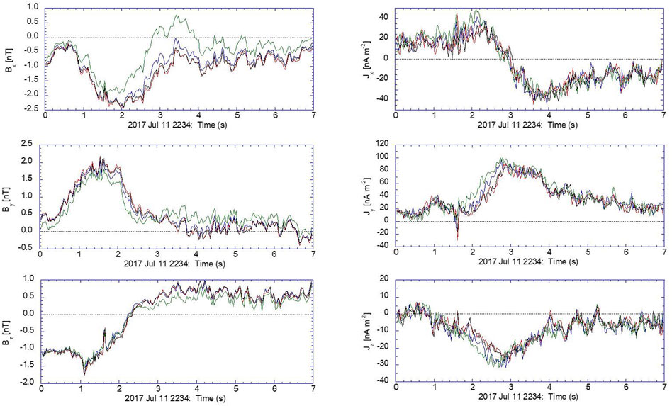
FIGURE 1. Measurements from the four MMS spacecraft (MMS1, MMS2, MMS3, MMS4) on 11 July 2017 showing (left) the measured magnetic field B^=(Bx,By,Bz) from FGM (Russell et al., 2016) and (right) particle current density J^=(Jx,Jy,Jz) from FPI (Pollock et al., 2016) in GSE coordinates.

Error Consideration and Quality Indicators

Note that the measurement errors here include uncertainties in both the instrumentation and subsequent processing of the data. However, the random errors in Eq. 8 are associated with the unbiased instrument noise. Here, we estimate the errors by directly calculating the parameter variability included in the data series. In Figure 2, we show both the means (B0,J0) and the normalized standard deviations (σB,σJ) of the magnitudes for the measured B^ and J^ fields. The averages are taken over the four spacecraft and over moving windows with widths of 7, 11, and 15 time steps, respectively. The calculated B0 is approximately equal to the characteristic value of the temporal mean of the magnetic field B00 defined in Supplementary Eq. A1. It is noted that the mean fields are not noticeably sensitive to the width of the moving window. This implies that the sampling rate of the measurements is high enough to resolve the temporal variability of the fields. It is also noted from Figure 2 that there is no systematic variation of σB with respect to B0, whereas σJ is inversely proportional to J0. The weighting factor wA in Eq. 6 is proportional to the σB2/σJ2 parameter that can be calculated from the values shown in the figure. The weighting factors (wB,wC) are prescribed to (1,0) for the default setting of the reconstruction model. Note that setting wB=1 here also means that we give no preference between the model-measurement differences L0 and the model departures LB. To set the final model parameter σ used in Eq. 8, we note that σB directly derived from the measured B^ contains both the unbiased random errors required for the construction of εσ in Eq. 8 and possibly also the biased errors associated with the parameter retrieval and data processing issues. In addition, a smaller σ in the random loss function y will yield a more numerically accurate solution, though its usefulness may be limited by the measurement errors; any numerical accuracy achieved that is higher than the measurement errors after setting σ0 does not contain additional information as the results are ultimately limited by the uncertainty in the measurements. As a result, our default setting for σ in the algorithm as shown in Eq. 8b takes a conservative value of σ=0.1σ¯B, where σ¯B is the time-averaged standard deviation of B^ as shown in Figure 2A.

FIGURE 2
www.frontiersin.org

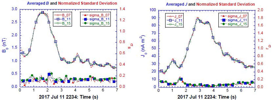
FIGURE 2. Mean and normalized standard deviation fields derived from the MMS measurements. The means and standard deviations are calculated on a moving window with a width of 7 (red), 11 (blue), and 15 (green) time steps, respectively. Panels (A) and (B) correspond to the B field and J field, respectively.

Given model parameters {B0i,C0i,j,D0i,jk}, a smooth 3D solution for (B,J) can be plotted to be visulized. But before addressing these visualizations, we begin our discussions here with evaluations of the quality factors associated with these results. In Figure 3, we show the relative differences of the fields (B,J) reconstructed at every time step based on the MMS-measured fields (B^,J^) shown in Figure 1. The indices (γB,γJ) can be considered as the normalized loss function components (LO,LA) corresponding to the model-measurement differences, which can be used as a set of accuracy indicators of the reconstruction model and are defined as:

γB=α=14i=13[Bi(rα)B^α,i]2α=14i=13B^α,i2and(9a)
γJ=α=14i=13[Ji(rα)J^α,i]2α=14i=13J^α,i2.(9b)

FIGURE 3
www.frontiersin.org

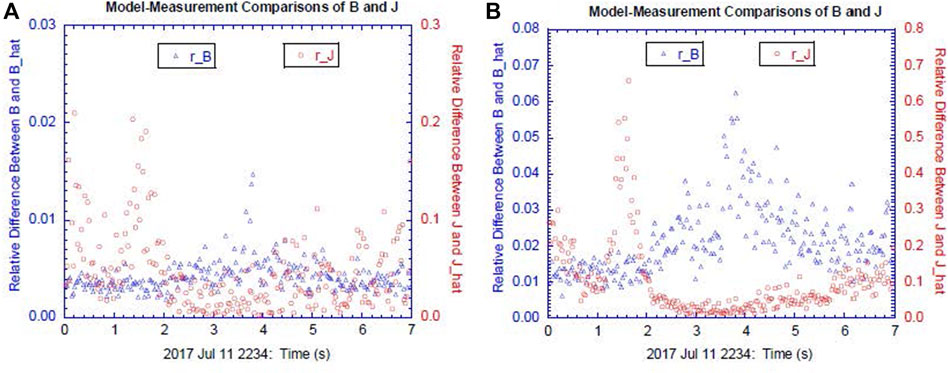
FIGURE 3. Relative differences (γB,γJ) of the reconstructed (B,J) fields based on MMS measurements shown in Figure 1. Panels (A) and (B) correspond to two cases of a standard setting of σ in Eq. 8 with σ=0.1σ¯B and an alternative setting of σ=σ¯B, respectively.

The results from a pair of reconstructions with σ=0.1σ¯B and σ=σ¯B, respectively, are presented in Figure 3. The default setting, which has a smaller measurement noise of σ=0.1σ¯B, yields a more accurate reconstruction field as characterized by smaller indices (γB,γJ). On the other hand, if the measurement noise in the loss function y amounts to σ¯B, such that σσ¯B0.1 as shown in Figure 2, then, a numerical solution of B with γB<σ¯B can be considered to be an acceptable or valid solution. Our default setting of σ=0.1σ¯B leads to a numerical solution of B with γBσ¯B, which can be considered an accurate solution. It should also be noted that because of the existence of measurement errors in B^ (i.e., σ>0), a deterministic and idealized solution with γB0 is considered to be as accurate as one with γB<σ. Figure 3 shows that far greater errors exist in the modeled current density γJ than those in the magnetic field γB. This is largely expected since the modeled current density J is a quantity derived from the prescribed B field and contains fewer free parameters and therefore is expected to lead to greater errors in J than in B. This is another reason for us to set σ so that it is much smaller than σ¯B in Eq. 8, which yields a solution also with an acceptable error in the reconstructed J field. Comparison between the two panels in Figure 3 shows that the magnitude of the errors in the reconstruction model is sensitive to the measurement errors. This feature can be further confirmed by examining γJ variation with the time-dependent measurement errors. We note from Figure 2 that σJ changes more significantly with time than σB, which leads to a significant variation in the weighting factor wA. Figure 4 shows both wA(=σB2/σJ2) and γJ for a standard setting of σ=0.1σ¯B. The figure shows a negative correlation between wA and γJ. Since errors in B^ are nearly constant, Figure 4 shows a strong positive correlation between the errors in the measured J^ and the modeled J. Overall, Figures 24 show that the accuracy of the reconstructed fields from the stochastic optimization algorithm is limited by the measurement uncertainties, with more accurate measurements unsurprisingly resulting in a more accurate solution for the reconstruction based upon those measurements.

FIGURE 4
www.frontiersin.org

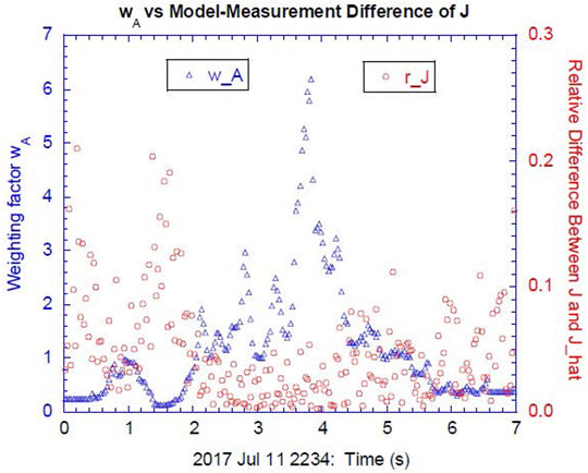
FIGURE 4. Weighting factor wA versus the relative difference γJ for the reconstructed current density J shown in Figure 3.

Unlike reconstruction models based on the GSR technique, where the reconstructed fields are mainly derived by various physical relations, the new ER model presented here is mainly data-driven, directly fitting the modeled fields to the measured fields. Since the design of the general loss function highlighted in Eqs. 6, 7 also contains a component of the model departures characterizing a few physical constraints, the validity of those constraints can be used as a measure of the quality of the ER model in addition to the two indices (γB,γJ) for measuring the accuracy of the solution. Here, one important constraint is the vanishing of the divergence of the magnetic field (B=0), which is also used as a constraint of the loss function component LB in Eq. 7. Dunlop et al. (1988) introduced an index of the ratio of the divergence to the vorticity of the magnetic field as a quality indicator to measure the robustness of the reconstructed current density J field. In Figure 5, we show the following two quality indicators Qmodel and Qcurl representing the ratio of the divergence to the vorticity of the magnetic field based on the reconstructed B field and the measured B^ field by curlometer technique, respectively. These are defined as

Qmodel=α=14(B)α2α=14i=13(×B|α,i)2and(10a)
Qcurl=[|B^||×B^|]curlometer.(10b)

FIGURE 5
www.frontiersin.org

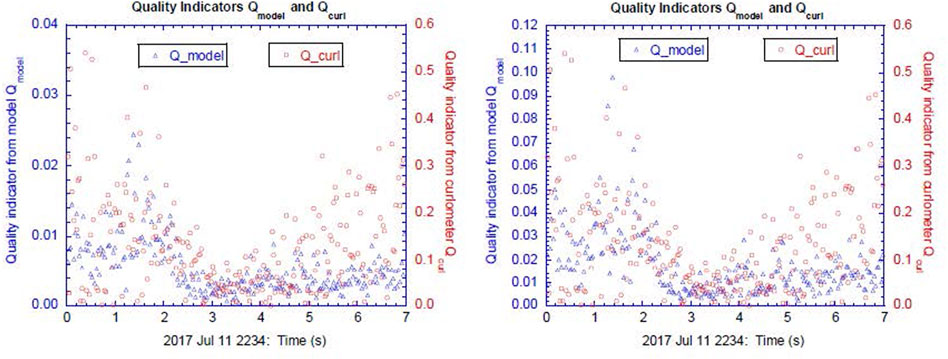
FIGURE 5. Quality indicators Qmodel and Qcurl representing the ratio of the divergence to the vorticity of the magnetic field based on the reconstructed B field and the measured B^ field by curlometer technique, respectively. The left and right panels correspond to two cases of a standard setting of σ in Eq. 8 with σ=0.1σ¯B and an alternative setting of σ=σ¯B, respectively.

In the above, Qmodel is calculated by evaluating B and ×B analytically based on the modeled B field at the four vertices, whereas Qcurl is calculated by evaluating the volume-averaged |B^| and |×B^| based on the measured B^ field following the schemes shown in Dunlop et al. (2002) and Middleton and Masson (2016). Note that Qcurl has also been used as an objective index that measures the quality of the J fields reconstructed from the curlometer technique (Dunlop et al., 2002). On the other hand, the index Qmodel defined in Eq. 10a measures the quality or robustness of both B and J fields derived from the ER model. Figure 5 shows that typically Qmodel0.01 for a standard setting of the model parameter σ=0.1σ¯B, whereas the typical values of Qcurl are much greater, Qcurl0.1. Since Qcurl is calculated directly by a linear approximation from the measured B^ field, it contains errors from both the linear approximation and measurement errors (Dunlop et al., 1988; Dunlop et al., 2002). Comparison between the two panels in Figure 5 also shows that the increase in the measurement errors by changing σ=0.1σ¯B to σ=σ¯B only increases the quality indicator Qmodel by a factor of ∼3 (note the changed scale on the ordinate between the two panels for just the “model” result, not the “curl” result). The relation of QmodelQcurl is still valid for σ=σ¯B. As a result, we can conclude based on Figure 5 that the uncertainties in the reconstructed fields based on the MMS-measured B^ near the EDR using the curlometer technique are mostly contributed by the linear approximation used in the technique. It should be pointed out that when an ER model is formulated and solved as an even-determined problem based on the traditional least-squares method, one may impose a condition of vanishing Qmodel everywhere (Qmodel0). In this case, an alternative constraint corresponding to model departures, say, a vanishing variance of the modeled B field in a particular diretion M, i.e., 2B/M2=0, needs to be introduced into the reconstruciton model (e.g., Torbert et al., 2020).

We now turn to the loss function component LC. The default setting of the weighting factors is (wB,wC)=(1,0). This means that the constraint of the precise physical relation of B=0 is fully utilized whereas the constraint of matching the modeled current components to the ones derived from the curlometer technique on the tetrahedron faces is neglected. Again, setting wB=1 here also means that we give no preference between two sets of constraints of the model-measurement differences and the model departures. Our analysis of the quality indicators (Qmodel,Qcurl) derived from the runs without LC shown in Figure 5 can be considered as a rationale for the default setting of wC=0. It is noted that the curlometer technique developed in Dunlop et al. (1988) and Middleton and Masson (2016) applies a linear approximation to the entire volume of the tetrahedron, whereas in LC the linear approximation applies only to the four individual tetrahedron faces. Hence, it is worthwhile examining quantitatively the effect of the loss function component LC on the performance of the reconstruction model. In Figure 6, we show the indices (rB,rJ) and the quality indicators (Qmodel,Qcurl) for a sensitivity run of the reconstruction model with all parameters in default settings, except wC that is set to 1. Comparing Figure 6A with Figure 3A, we find that the inclusion of LC significantly reduces the accuracy of the reconstructed fields. This is expected because the inclusion of LC not only introduces a linear approximation in the calculation of the current density J from the magnetic field B, but also enhances the degree of over-determination of the model. Both of these are expected to increase the errors of a least-squares solution. Comparing Figure 6B with Figure 5A on the modeled quality indicators Qmodel derived from different runs underscores the same conclusion—i.e., that the inclusion of LC makes the model performance worse. However, Figure 6B also shows that Qmodel is still significantly smaller than Qcurl (note the different scales), indicating that a linear approximation in a loss function component only partially affects the model performance. This sensitivity investigation of setting wC=1 also demostrates the flexibility of the new ER model that directly minimizes the general loss function with its components being able to be included or excluded without changing the model framework.

FIGURE 6
www.frontiersin.org

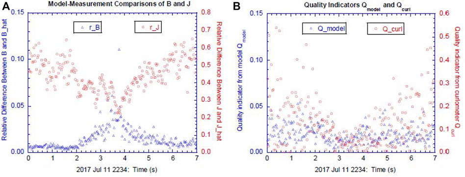
FIGURE 6. (A) Relative differences (γB,γJ) and (B) quality indicators (Qmodel,Qcurl) for a sensitivity run with weighting factors wB and wC being both set to 1: (wB,wC)=(1,1).

At this stage, it is also interesting to examine a largely under-determined setting of excluding both LB and LC in the generalized loss function L by setting (wB,wC)=(0,0) in Eq. 6. There are only twenty-four (24) constraints in LO and LA, all given by the MMS measurements, whereas the reconstruction model contains thirty (30) model parameters that need to be determined. Hence, the problem is largely under-determined and the solution cannot be uniquely solved. For a stochastic optimization, such as the one based on the SPSA method, there is no fundamental difference in the non-uniqueness of the solution either due to the lack of constraints or due to random errors in the loss function. In other words, the unknown parameters for the reconstruction model can always be formally solved by minimizing the generalized loss function y in Eq. 8. Figure 7 shows the indices (γB,γJ) and the quality indicators (Qmodel,Qcurl) for a sensitivity run of the reconstruction model that sets (wB,wC)=(0,0). We note from Figure 7A that the relative differences between the modeled and measured fields (γB,γJ) are much less than those shown in Figures 3A, 6A. However, the quality indicator Qmodel shown in Figure 7B is much greater than those derived by any approach shown above including Qcurl derived by the curlometer technique. Figure 7 shows that even though one can construct an empirical model that leads to a very good fit between the modeled and the measured fields at the prescribed spatial points, the fields may not necessarily satisfy some physical relations, such as B=0. This is due to the following two facts: 1) the fields contain errors, either in the measured field or in the modeled field derived from the measurements and 2) the numerical evaluation of the physical relation based on the discrete measurements involves a small difference between two large quantities. The divergence of a vector field contains two components of variation corresponding to variations in the magnitude and direction of the vector. For a deformation vector field that is mainly confluent-diffluent—i.e., divergence is mainly caused by the change in direction—the calculation of the divergence of the vector field generally involves a small difference of two large quantities (e.g., Holton, 2004). In this case, small errors in the B field will be greatly amplified in calculating B unless an additional constraint or assumption of B=0, or |B| being small, is explicitly included in the model or algorithm development. A similar assumption of “charge neutrality” in plasma physics is also used as an explicitly imposed constraint in developing various MHD models (e.g., Gurnett and Bhattacharjee, 2005).

FIGURE 7
www.frontiersin.org

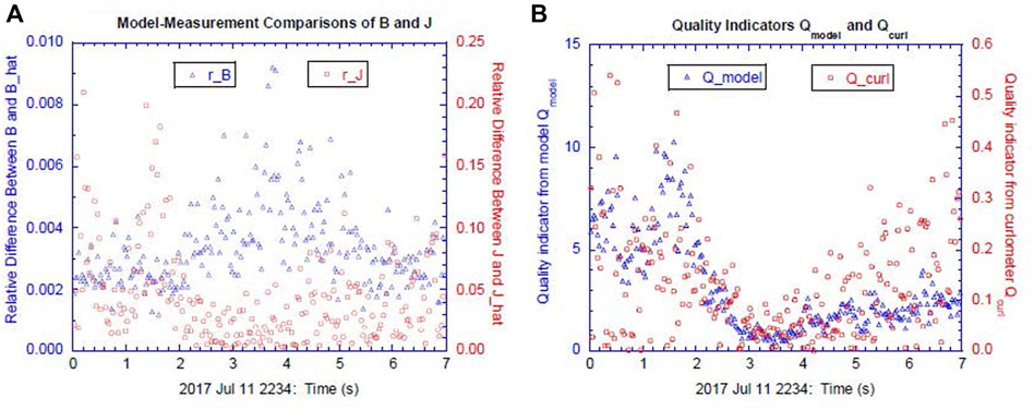
FIGURE 7. (A) Relative differences (γB,γJ) and (B) quality indicators (Qmodel,Qcurl) for a sensitivity run with weighting factors wB and wC being both set to 0: (wB,wC)=(0,0).

The other more important implication of this test run for a largely under-determined setting with only 24 constraints for a 30-parameter reconstruction model is that the current ER model can be directly applied to reconstructing fields with a set of incomplete measurements. The stochastic optimization algorithms can solve for model parameters under the same algorithmic framework regardless whether the problem is over- or under-determined. For example, for a default setting of the current ER model with 33 constraints, the algorithm can be directly applied to an incomplete set of MMS measurements if the (B^,J^) measurements from one spacecraft are not available. Under such a circumstance, the same algorithm with 27 (= 33−6) constraints will produce a reconstruction field (B,J) that fits the measured (B^,J^) at three vertices having available measurements plus B=0 being satisfied at all four vertices, all within the measurement errors. The results shown in Figure 7 also suggest that the deterioration of the reconstructed fields due to lack of the needed constraints is gradual. On the other hand, the algorithm based on the traditional least-squares method that solves a set of linear algebraic equations (e.g., Torbert et al., 2020) becomes inapplicable once the problem changes from an even- to under-determined one.

The Reconstructed Fields

We now present the reconstructed fields based on the MMS measurements shown in Figure 1. A reconstruction model can be developed in either an L-M-N coordinate system derived from the minimum variance analysis or in a fixed system, such as GSE that is used in the present reconstruction model. One purpose of adopting the L-M-N coordinate system to develop a reconstruction model is to take advantage of the ability to neglect changes in the minimum variance direction to convert a slightly under-determined problem into an even-determined one (Denton et al., 2020; Torbert et al., 2020). When the reconstructed field varies rapidly with time, the constructed L-M-N coordinate may also change accordingly. Under such a circumstance, the reconstructed fields at different time instances cannot be directly compared with each other. Our reconstruction model based on the SPSA stochastic optimization method can automatically accommodate an over-determined or under-determined setting of the model as discussed above. As a result, the fields reconstructed at different temporal instances but on the common, fixed GSE coordinate system can be directly compared.

We present the reconstructed fields in a local GSE coordinate X-Y-Z such that

(X,Y,Z)=(X,Y,Z)(X0,Y0,Z0),(11)

where X-Y-Z define the generic GSE coordinate system and (X0,Y0,Z0) = (1.373×105,2.70×104,2.32×104) km is determined by the satellite constellation, which corresponds to the GSE coordinate of the mean barycenter averaged over the measurement time shown in Figure 1. In Figure 8, we show the reconstructed B fields projected into and its magnitude |B| (=B12+B22+B32, in nT) evaluated on the X-Z plane of Y = 0 at six time instances of (a) t=1.172 s, (b) t=1.904 s, (c) t=2.636 s, (d) t=3.368 s, (e) t=4.100 s, and (f) t=4.833 s after 22:34 UT. The figure shows that both the magnetic configuration and the intensity of the magnetic field change noticeably with time. The reconnection region is characterized by a weak |B| and a reversal of the orientation (or a near anti-parallization) of the B vectors across the region. It is noted that a weak |B| also means a weak confinement to the motions of energetic electrons. This will lead to localized very fine-scale energy spectra and angular distributions that could be correlated with the remote magnetic topologies through the gyro-sounding process as revealed by the data from the Fly’s Eye Energetic Particle Spectrometer (FEEPS) onboard the MMS spacecrafts (Cohen et al., 2021; Turner et al., 2021). The development and evolvement of these two features can be easily identified in this figure. To provide a better view on the development of the reconnection region, we show in Figure 9A the superimposed B fields at two neighboring time instances of t=2.636 s and t=3.368 s on the same plot. The figure shows the development of an anti-parallel B field having a nearly opposite direction and an equal magnitude with a significantly weak B field sandwiched between the two regions at t=3.368 s and especially in the region of X>0. Though the reconstruction in the present model is under the X-Y-Z coordinate whereas the reconstruction in Torbert et al. (2020) was presented in the L-M-N coordinate, the configuration of the reconstructed B-field shown in Figure 9A is qualitatively similar to that shown in Torbert et al. (2020). Figure 9B shows the corresponding cross tail current J on the Y-Z plane of X = 0 that shows a significant intensification in its magnitude due to the development of the reconnection event.

FIGURE 8
www.frontiersin.org

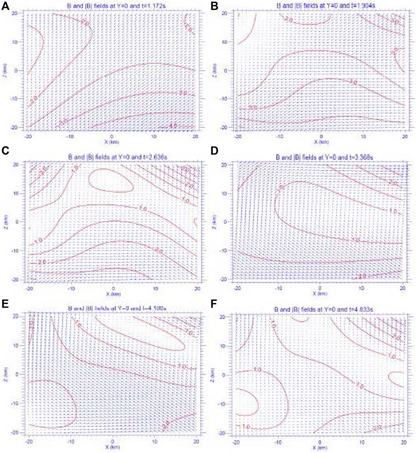
FIGURE 8. Modeled B fields projected into and its magnitude |B| (in nT) evaluated on the X-Z plane of Y = 0 at six time instances of (A) t=1.172 s, (B) t=1.904 s, (C) t=2.636 s, (D) t=3.368 s, (E) t=4.100 s, and (F) t=4.833 s after 22:34 UT on 11 July 2017.

FIGURE 9
www.frontiersin.org

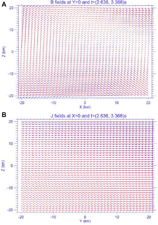
FIGURE 9. (A) Modeled B fields projected into the X-Z plane of Y = 0 at two times of t=2.636 s (blue) and t=3.368 s (red) after 22:34 UT on 11 July 2017. (B) Modeled J fields projected into the Y-Z plane of X = 0 at the same two instances as in panel (A). A significant intensification in J fields at t=3.368 s as indicated by a plot with dominant red arrows.

Conclusion

A new ER model for the 3D magnetic field and plasma current field has been developed by use of a stochastic optimization method called SPSA. This reconstruction model adopts an empirical approach by fitting the prescribed analytic functions for the magnetic and plasma fields to the point-wise measurements from a constellation of satellites with a set of physical constraints determined by the MHD equations. The fitness is defined by a general loss function that consists of the model-measurement differences and the model departures from linear or nonlinear physical constraints. The new ER model directly minimizes the loss function using a stochastic optimization method called SPSA algorithm for which the effect of the random measurement errors is also included. We presented the concrete steps of how to implement this ER model to a special case of having the MMS-measured fields (B^,J^) combined with a set of physical constraints corresponding to an ideal MHD system of Eqs. 1a, b, which has been extensively investigated by traditional least-squares method (e.g., Denton et al., 2020; Torbert et al., 2020). Most SPSA applications contain the loss functions that only involve the difference between the modeled and measured quantities (e.g., Chin, 1999; Spall, 2003). On the other hand, the constraints contained in the generalized loss function (6) include not only the model-measurement differences but also the model departures derived from the physical constraints Eqs. 1a, b, which in turn characterizes the physical robustness of the fields reconstructed by an empirical model.

We have introduced the indices (rB,rJ) in Eq. 9 that calculate the relative differences between the modeled (B,J) fields and the measured (B^,J^) fields. This set of indices (γB,γJ) provides an objective measure of the accuracy to the modeled fields. In addition, the concept of the quality indicator Qcurl introduced in Dunlop et al. (1988) has been extended to a new model quality indicator Qmodel shown in Eq. 10. This index provides an objective measure to the robustness of the modeled field in terms of its physical property of B=0. These two sets of new indices are respectively associated with the two sets of constraints of model-measurement differences and the model departures used in designing the general loss function for the new ER model. The new ER model was applied to the measurements of an EDR observed by the MMS mission (Torbert et al., 2018). By conducting various sensitivity investigations of the reconstruction model, we were able to examine the sources of the errors in the reconstructed fields previously noted by the curlometer technique. It is now found that the errors in the plasma current density calculated directly from the measured magnetic fields based on curlometer technique were mostly contributed from the linear approximation to a nonlinear configuration of the 3D magnetic fields. A more comprehensive nonlinear ER model that uses Eqs. 13 with point-wise measurements of (B, J) and (U, E) fields and effectively includes the effects of plasma resistivity contained in Eqs. 2, 3 near the EDRs will be presented in our future investigations.

Data Availability Statement

The original contributions presented in the study are included in the article/Supplementary Material, further inquiries can be directed to the corresponding author.

Author Contributions

XZ: Proposed the original idea, developed the model, and wrote the paper. IC: Provided the data, refined the idea, and revised the paper. BM: Refined the idea and revised the paper. RN: Refined the idea and revised the paper. DT: Refined the idea through various discussions. RT: Refined the idea.

Funding

This research was supported by the Magnetospheric Multiscale (MMS) mission of NASA’s Science Directorate Heliophysics Division via subcontract to the Southwest Research Institute (NNG04EB99C) and NASA Grant NNX10AB84G.

Conflict of Interest

The authors declare that the research was conducted in the absence of any commercial or financial relationships that could be construed as a potential conflict of interest.

Publisher’s Note

All claims expressed in this article are solely those of the authors and do not necessarily represent those of their affiliated organizations, or those of the publisher, the editors and the reviewers. Any product that may be evaluated in this article, or claim that may be made by its manufacturer, is not guaranteed or endorsed by the publisher.

Acknowledgments

Constructive comments on SPSA applications from James C. Spall and Richard Denton are greatly appreciated. We also thank Daniel J. Gershman and others on MMS team for the FPI current density and magnetic field measurements used in this paper. Constructive comments from two reviewers are also appreciated.

Supplementary Material

The Supplementary Material for this article can be found online at: https://www.frontiersin.org/articles/10.3389/fspas.2022.878403/full#supplementary-material

References

Axelsson, O. (1996). Iterative Solution Methods. Cambridge: Cambridge University Press, 654.

Google Scholar

Bhatnagar, S., Prasad, H. L., and Prashanth, L. A. (2013). Stochastic Recursive Algorithms for Optimization - Simultaneous Perturbation Method. New York: Springer, 302.

Google Scholar

Boyd, T. J., and Sanderson, J. J. (2003). The Physics of Plasmas. Cambridge: Cambridge University Press, 532.

Google Scholar

Burch, J. L., Moore, T. E., Torbert, R. B., and Giles, B. L. (2016). Magnetospheric Multiscale Overview and Science Objectives. Space Sci. Rev. 199, 5–21. doi:10.1007/s11214-015-0164-9

CrossRef Full Text | Google Scholar

Chanteur, G. (1998). “Spatial Interpolation for Four Spacecraft: Theory,” in Analysis Methods for Multi-Spacecraft Data. Editors G. Paschmann, and P. W. Daly (Bern, Switzerl, and Paris, France: The International Space Science InstituteEuropean Space Agency), 395–418. Chap. 12.

Google Scholar

Chin, D. C. (1999). Simultaneous Perturbation Method for Processing Magnetospheric Images. Opt. Eng. 38, 606–611. doi:10.1117/1.602104

CrossRef Full Text | Google Scholar

Chong, E. K. P., and Zak, S. H. (2001). An Introduction to Optimization. Second Edition. New York: John Wiley & Sons, 476.

Google Scholar

Cohen, I. J., Turner, D. L., Mauk, B. H., Bingham, S. T., Blake, J. B., Fennell, J. F., et al. (2021). Characteristics of Energetic Electrons Near Active Magnetotail Reconnection Sites: Statistical Evidence for Local Energization. Geophys. Res. Lett. 48, e2020GL090087. doi:10.1029/2020GL090087

CrossRef Full Text | Google Scholar

Denton, R. E., Torbert, R. B., Hasegawa, H., Dors, I., Genestreti, K. J., Argall, M. R., et al. (2020). Polynomial Reconstruction of the Reconnection Magnetic Field Observed by Multiple Spacecraft. J. Geophys. Res. Space Phys. 125, e2019JA027481. doi:10.1029/2019JA027481

CrossRef Full Text | Google Scholar

Dunlop, M. W., Balogh, A., Glassmeier, K.-H., and Robert, P. (2002). Four-point Cluster Application of Magnetic Field Analysis Tools: The Curlometer. J. Geophys. Res. 107 (A11), 1384. doi:10.1029/2001JA005088

CrossRef Full Text | Google Scholar

Dunlop, M. W., Southwood, D. J., Glassmeier, K.-H., and Neubauer, F. M. (1988). Analysis of Multipoint Magnetometer Data. Adv. Space Res. 8, 273–277. doi:10.1016/0273-1177(88)90141-x

CrossRef Full Text | Google Scholar

Gurnett, D. A., and Bhattacharjee, A. (2005). Introduction to Plasma Physics – with Space and Laboratory Applications. Cambridge: Cambridge University Press, 452.

Google Scholar

Harvey, C. C. (1998). “Spatial Gradients and the Volumetric Tensor,” in Analysis Methods for Multi-Spacecraft Data. Editors G. Paschmann, and P. W. Daly (Bern, Switzerl, and Paris, France: The International Space Science InstituteEuropean Space Agency), 307–322. Chap. 12.

Google Scholar

Hasegawa, H., Sonnerup, B. U. Ö., Dunlop, M. W., Balogh, A., Haaland, S. E., Klecker, B., et al. (2004). Reconstruction of Two-Dimensional Magnetopause Structures from Cluster Observations: Verification of Method. Ann. Geophys. 22, 1251–1266. doi:10.5194/angeo-22-1251-2004

CrossRef Full Text | Google Scholar

Hasegawa, H., Sonnerup, B. U. Ö., Klecker, B., Paschmann, G., Dunlop, M. W., and Rème, H. (2005). Optimal Reconstruction of Magnetopause Structures from Cluster Data. Ann. Geophys. 23, 973–982. doi:10.5194/angeo-23-973-2005

CrossRef Full Text | Google Scholar

Holton, J. R. (2004). An Introduction to Dynamic Meteorology. Fourth Edition. New York: Elsevier Academic Press, 535.

Google Scholar

Menke, W. (1989). Geophysical Data Analysis: Discrete Inverse Theory. Revised Edition. New York: Academic Press, 289.

Google Scholar

Middleton, H., and Masson, A. (2016). The Curlometer Technique: A Beginner’s Guide. CSA Technical Note. ESDC-CSA-TN-0001. Madrid, Spain: European Space Astronomy Centre, 19.

Google Scholar

Pollock, C., Moore, T., Jacques, A., Burch, J., Gliese, U., Saito, Y., et al. (2016). Fast Plasma Investigation for Magnetospheric Multiscale. Space Sci. Rev. 199, 331–406. doi:10.1007/s11214-016-0245-4

CrossRef Full Text | Google Scholar

Press, W. H., Teukolsky, S. A., Vetterling, W. T., and Flannery, B. P. (1992). Numerical Recipes in Fortran. The Arts of Scientific Computing. Second Edition. Cambridge: Cambridge University Press, 963.

Google Scholar

Priest, E. (2016). “MHD Structures in Three-Dimensional Reconnection,” in Magnetic Reconnection – Concepts and Applications. Editors W. Gonzalez, and E. Parker (Switzerland: Springer), 101–142. doi:10.1007/978-3-319-26432-5_3

CrossRef Full Text | Google Scholar

Robert, P., Roux, A., Harvey, C. C., Dunlop, M. W., Daly, P. W., and Glassmeier, K. H. (1998). “Tetrahedron Geometric Factors,” in Analysis Methods for Multi-Spacecraft Data. Editors G. Paschmann, and P. W. Daly (Bern, Switzerl, and Paris, France: The International Space Science InstituteEuropean Space Agency), 323–348. Chap. 13.

Google Scholar

Roelof, E. C., Mauk, B. H., and Meier, R. R. (1993). Simulations of EUV and ENA Magnetospheric Images Based on the Rice Convection Model. Proc. Spie, Instrumentation Magnetospheric Imagery 2008, 202–213.

Google Scholar

Russell, C. T., Anderson, B. J., Baumjohann, W., Bromund, K. R., Dearborn, D., Fischer, D., et al. (2016). The Magnetospheric Multiscale Magnetometers. Space Sci. Rev. 199, 189–256. doi:10.1007/s11214-014-0057-3

CrossRef Full Text | Google Scholar

Scudder, J. D. (2016). “Collisionless Reconnection and Electron Demagnetization,” in Magnetic Reconnection – Concepts and Applications. Editors W. Gonzalez, and E. Parker (Switzerland: Springer), 33–100. doi:10.1007/978-3-319-26432-5_2

CrossRef Full Text | Google Scholar

Sonnerup, B. U. Ö., and Guo, M. (1996). Magnetopause Transects. Geophys. Res. Lett. 23, 3679–3682. doi:10.1029/96gl03573

CrossRef Full Text | Google Scholar

Sonnerup, B. U. Ö., Hasegawa, H., Denton, R. E., and Nakamura, T. K. M. (2016). Reconstruction of the Electron Diffusion Region. J. Geophys. Res. Space Physics 121, 4279–4290. doi:10.1002/2016JA022430

CrossRef Full Text | Google Scholar

Sonnerup, B. U. Ö., and Teh, W.-L. (2008). Reconstruction of Two-Dimensional Coherent MHD Structures in a Space Plasma: The Theory. J. Geophys. Res. 113. doi:10.1029/2007JA012718

CrossRef Full Text | Google Scholar

Spall, J. C. (2000). Adaptive Stochastic Approximation by the Simultaneous Perturbation Method. IEEE Trans. Automat. Contr. 45, 1839–1853. doi:10.1109/tac.2000.880982

CrossRef Full Text | Google Scholar

Spall, J. C. (1998a). An Overview of the Simultaneous Perturbation Method for Efficient Optimization. Johns Hopkins APL Tech. Dig. 19, 482–492.

Google Scholar

Spall, J. C. (1998b). Implementation of the Simultaneous Perturbation Algorithm for Stochastic Optimization. IEEE Trans. Aerosp. Electron. Syst. 34 (3), 817–823. doi:10.1109/7.705889

CrossRef Full Text | Google Scholar

Spall, J. C. (2003). Introduction to Stochastic Search and Optimization: Estimation, Simulation, and Control. New York: John Wiley & Sons, 595.

Google Scholar

Spall, J. C. (1992). Multivariate Stochastic Approximation Using a Simultaneous Perturbation Gradient Approximation. IEEE Trans. Automat. Contr. 37, 332–341. doi:10.1109/9.119632

CrossRef Full Text | Google Scholar

Sturrock, P. A. (1994). Plasma Physics: An Introduction to the Theory of Astrophysical, Geophysical and Laboratory Plasmas. Cambridge: Cambridge University Press, 335.

Google Scholar

Torbert, R. B., Burch, J. L., Phan, T. D., Hesse, M., Argall, M. R., Shuster, J., et al. (2018). Electron-scale Dynamics of the Diffusion Region during Symmetric Magnetic Reconnection in Space. Science 362 (6421), 1391–1395. doi:10.1126/science.aat2998

PubMed Abstract | CrossRef Full Text | Google Scholar

Torbert, R. B., Dors, I., Argall, M. R., Genestreti, K. J., Burch, J. L., Farrugia, C. J., et al. (2020). A New Method of 3‐D Magnetic Field Reconstruction. Geophys. Res. Lett. 47, e2019GL085542. doi:10.1029/2019gl085542

CrossRef Full Text | Google Scholar

Tsyganenko, N. A., and Sitnov, M. I. (2007). Magnetospheric Configurations from a High-Resolution Data-Based Magnetic Field Model. J. Geophys. Res. 112. doi:10.1029/2007JA012260

CrossRef Full Text | Google Scholar

Turner, D. L., Cohen, I. J., Bingham, S. T., Stephens, G. K., Sitnov, M. I., Mauk, B. H., et al. (2021). Characteristics of Energetic Electrons Near Active Magnetotail Reconnection Sites: Tracers of a Complex Magnetic Topology and Evidence of Localized Acceleration. Geophys. Res. Lett. 48, e2020GL090089. doi:10.1029/2020GL090089

CrossRef Full Text | Google Scholar

Yamada, M., Yoo, J., and Zenitani, S. (2016). “Energy Conversion and Inventory of a Prototypical Magnetic Reconnection Layer,” in Magnetic Reconnection – Concepts and Applications. Editors W. Gonzalez, and E. Parker (Switzerland: Springer), 143–179. doi:10.1007/978-3-319-26432-5_4

CrossRef Full Text | Google Scholar

Zhu, X., and Lui, A. T. Y. (2012). Reconstruction of Neighboring Plasma Environment along a Satellite Path by a Barotropic Plasma Model. J. Atmos. Solar-Terrestrial Phys. 77, 46–56. doi:10.1016/j.jastp.2011.11.005

CrossRef Full Text | Google Scholar

Zhu, X., and Spall, J. C. (2002). A Modified Second-Order SPSA Optimization Algorithm for Finite Samples. Int. J. Adapt. Control. Signal. Process. 16, 397–409. doi:10.1002/acs.715

CrossRef Full Text | Google Scholar

Keywords: stochastic optimization, empirical reconstruction model, magnetospheric reconnection, simultaneous perturbation stochastic approximation, loss function

Citation: Zhu X, Cohen IJ, Mauk BH, Nikoukar R, Turner DL and Torbert RB (2022) A New Three-Dimensional Empirical Reconstruction Model Using a Stochastic Optimization Method. Front. Astron. Space Sci. 9:878403. doi: 10.3389/fspas.2022.878403

Received: 18 February 2022; Accepted: 07 April 2022;
Published: 09 May 2022.

Edited by:

Olga Verkhoglyadova, NASA Jet Propulsion Laboratory (JPL), United States

Reviewed by:

Bogdan Hnat, University of Warwick, United Kingdom
Yasuhito Narita, Austrian Academy of Sciences (OeAW), Austria

Copyright © 2022 Zhu, Cohen, Mauk, Nikoukar, Turner and Torbert. This is an open-access article distributed under the terms of the Creative Commons Attribution License (CC BY). The use, distribution or reproduction in other forums is permitted, provided the original author(s) and the copyright owner(s) are credited and that the original publication in this journal is cited, in accordance with accepted academic practice. No use, distribution or reproduction is permitted which does not comply with these terms.

*Correspondence: Xun Zhu, xun.zhu@jhuapl.edu

Disclaimer: All claims expressed in this article are solely those of the authors and do not necessarily represent those of their affiliated organizations, or those of the publisher, the editors and the reviewers. Any product that may be evaluated in this article or claim that may be made by its manufacturer is not guaranteed or endorsed by the publisher.