
95% of researchers rate our articles as excellent or good
Learn more about the work of our research integrity team to safeguard the quality of each article we publish.
Find out more
METHODS article
Front. Astron. Space Sci. , 18 May 2022
Sec. Space Physics
Volume 9 - 2022 | https://doi.org/10.3389/fspas.2022.866455
This article is part of the Research Topic Sources and Propagation of Ultra-Low Frequency Waves in Planetary Magnetospheres View all 9 articles
 H. George1*
 A. Osmane1
 E. K. J. Kilpua1
 S. Lejosne 2
 L. Turc1
 M. Grandin1
 M. M. H. Kalliokoski1
 S. Hoilijoki1
 U. Ganse1
 M. Alho1M. Battarbee1M. Bussov1M. Dubart1A. Johlander1,3T. Manglayev1K. Papadakis1
 Y. Pfau-Kempf1J. Suni1V. Tarvus1
 H. Zhou1
 M. Palmroth1,4
Radial diffusion coefficients quantify non-adiabatic transport of energetic particles by electromagnetic field fluctuations in planetary radiation belts. Theoretically, radial diffusion occurs for an ensemble of particles that experience irreversible violation of their third adiabatic invariant, which is equivalent to a change in their Roederer L* parameter. Thus, the Roederer L* coordinate is the fundamental quantity from which radial diffusion coefficients can be computed. In this study, we present a methodology to calculate the Lagrangian derivative of L* from global magnetospheric simulations, and test it with an application to Vlasiator, a hybrid-Vlasov model of near-Earth space. We use a Hamiltonian formalism for particles confined to closed drift shells with conserved first and second adiabatic invariants to compute changes in the guiding center drift paths due to electric and magnetic field fluctuations. We investigate the feasibility of this methodology by computing the time derivative of L* for an equatorial ultrarelativistic electron population travelling along four guiding center drift paths in the outer radiation belt during a 5 minute portion of a Vlasiator simulation. Radial diffusion in this simulation is primarily driven by ultralow frequency waves in the Pc3 range (10–45 s period range) that are generated in the foreshock and transmitted through the magnetopause to the outer radiation belt environment. Our results show that an alternative methodology to compute detailed radial diffusion transport is now available and could form the basis for comparison studies between numerical and observational measurements of radial transport in the Earth’s radiation belts.
Wave activity plays a central role in the dynamic evolution of electron distributions in the radiation belts. Different waves affect different electron populations, and can cause their transport (e.g. radial diffusion, Parker, 1960), enhancement (e.g. local acceleration, Reeves et al., 2013) or loss (e.g. pitch angle scattering into the upper atmosphere, Kennel and Petschek, 1966). Understanding the effect of a given wave on electron populations with a given kinetic energy, equatorial pitch angle and magneticdrift shell is an essential component in quantifying the dynamical evolution of the radiation belts and the impact that energetic particles have on satellites and communication systems.
Radial diffusion is the process by which particles move to different drift shells due to the violation of the third adiabatic invariant by time-varying electromagnetic fields (Parker, 1960). Ultralow frequency (ULF) waves are a key driver of radial diffusion in the Earth’s magnetosphere (Su et al., 2015). The ULF waves are divided into five period bands (Pc1: 0.2–5 s, Pc2: 5–10 s, Pc3: 10–45 s, Pc4: 45–150 s and Pc5: 150–600 s, Jacobs et al., 1964), with drift resonant radial diffusion of outer radiation belt electrons primarily driven by ULF Pc4 and Pc5 waves. This is because these wave periods correspond to the drift periods of energetic electrons in the outer radiation belt and can therefore efficiently violate the third adiabatic invariant of these populations. Irreversible transport across drift shells is only possible in the presence of antisymmetric (magnetic local time, MLT, dependent) fluctuations, as the symmetric component of ULF waves drives equal radial transport of all particles in a given population and hence do not contribute to radial diffusion (Northrop, 1963; Fälthammar, 1965). Studies of radial diffusion require knowledge of the global electromagnetic field fluctuations in order to capture the effect of these antisymmetric ULF waves on particle populations throughout their drift motion.
A central focus of radial diffusion studies is determining the radial diffusion coefficients, which quantify the amount of radial diffusion that a particle population undergoes in given radiation belt conditions. Various models and expressions for the radial diffusion coefficients have been developed, beginning soon after the discovery of the radiation belts (e.g., Davis and Chang, 1962) and continuing until the present day (e.g., Sandhu et al., 2021). The radial diffusion coefficient is an input to the Fokker-Planck equation that describes the time evolution of a population’s distribution function (e.g. Davis and Chang, 1962; Schulz and Lanzerotti, 1974). As the Fokker-Planck formalism is in adiabatic space, calculating radial diffusion coefficients in adiabatic coordinates allows for more efficient evaluation of the time evolution of a population undergoing radial diffusion. It additionally captures the drift motion of particles in realistic (non-dipolar) geomagnetic fields. Therefore, the appropriate coordinate to evaluate the radial diffusion coefficients over is the third adiabatic invariant (see Lejosne and Kollmann, 2020, for further discussion). The third adiabatic invariant is proportional to the magnetic flux (Φ) enclosed by the guiding center drift path of the population, which is defined as the surface integral of the normal component of the magnetic field (B) through the surface (S) bounded by the guiding center drift path, so Φ = ∬SB ⋅ dS. We define the Roederer L-star (L*) coordinate absolute values from the magnetic flux as
(Roederer, 1967). In this equation, BE is the mean equatorial magnetic field at the Earth’s surface and RE is the mean radius of the Earth. We refer to radial diffusion coefficients evaluated in terms of L* as DL*L*. Many studies (e.g. Brautigam and Albert, 2000) instead use the McIlwain L-shell coordinate that corresponds to the equatorial radial distance of the drift shell in a dipole field (McIlwain, 1961) to compute the radial diffusion coefficients, which we here refer to as DLL. L-shell is numerically equal to L* evaluated with a dipolar background field, and evaluation of a non-dipolar geomagnetic field is significantly more complex than a dipole treatment, making L-shell significantly easier to compute than L*. There is however a significant difference between radial diffusion coefficients evaluated with dipolar and non-dipolar background fields (Cunningham, 2016), particularly at large radial distances and during geomagnetically active conditions, highlighting the importance of evaluating the radial diffusion coefficients over L* rather than L-shell.
The total change in L* at a single point on the drift path after a time T is
Antisymmetric wave activity drives radial diffusion, so ΔL*(T) is MLT dependent. We must evaluate the variations driving ΔL*(T) at all MLT along the drift path in order to capture the effect that this antisymmetry has on radial diffusion. We do this by computing the average over MLT, which we do here by evaluating the fluctuations of a general, MLT-dependent factor, f (MLT), at N points along the drift path at a given time and then computing the mean across these MLT points. The drift average, represented with the brackets ⟨⟩, is therefore defined as
The drift average of the squared change in L* will eventually grow linearly over time for a population undergoing radial diffusion. The time derivative
Rigorous calculation of L* requires global knowledge of the Earth’s magnetic field, and calculating the radial diffusion coefficient according to this definition requires good resolution of the electromagnetic fields in both time and MLT. There are currently significant limitations in our ability to determine the dynamics of the electromagnetic fields, using either observational data or simulations, that hampers radial diffusion research. Radial diffusion studies using satellite measurements (e.g. Brautigam et al., 2005; Ali et al., 2016) require a statistical model of the wave fields in order to calculate the global ULF wave activity and hence DLL, as satellites only provide local measurements of the electric and magnetic fields. Stormtime ULF wave activity is highly MLT dependent, in terms of both the wave power (e.g. Zhu and Kivelson, 1991; Anderson, 1994; Sandhu et al., 2021) and the occurrence rate (e.g. Kokubun et al., 1989; Nose et al., 1998; Dai et al., 2015). The afternoon (12 – 18 MLT) median power spectral density of ULF waves is typically orders of magnitude greater than the morning (06 – 12 MLT) values in the main and recovery phases of geomagnetic storms, likely due to excitation from ring current ions (Sandhu et al., 2021). Therefore, assuming that local satellite measurements are representative of the global wave activity can over/underestimate the true driving wave activity if the satellite is in a sector that happens to have high/low ULF activity respectively, leading to flawed estimates of the radial diffusion coefficients. Additionally, there are multiple sources of ULF waves in the inner magnetosphere, so observational studies are unable to evaluate the contribution of waves from a specific source to radiation belt radial diffusion. Magnetohydrodynamic (MHD) models have been used previously to calculate the radial diffusion coefficients in combination with test particle tracing codes (e.g. Elkington et al., 2002; Huang et al., 2010; Li et al., 2017). While this approach uses a fully specified global electromagnetic field, the use of test particle tracing is computationally costly as many individual particles must be traced to evaluate the response of an entire population to a given radiation belt environment. Other radial diffusion coefficient models are fully parametrized by ground-based measurements of the geomagnetic KP index (e.g. Brautigam and Albert, 2000; Ozeke et al., 2012, 2014; Ali et al., 2016), which is computationally inexpensive but can lead to significant underestimates of stormtime radial diffusion coefficients (Li et al., 2017; Olifer et al., 2019; Sandhu et al., 2021). Each of these approaches therefore has significant drawbacks, limiting our ability to understand and to quantify the role of ULF-driven radial diffusion on the outer radiation belt electron distribution.
In this study, we present a methodology to calculate the L* time derivative from a model that provides information on the global magnetic field topology, i.e. an MHD or a hybrid model. We demonstrate this methodology on the hybrid-Vlasov Vlasiator model (von Alfthan et al., 2014; Palmroth et al., 2018) and then demonstrate the application of this to the calculation of radial diffusion coefficients. This approach calculates the L* time derivative directly from the global electromagnetic field data provided by the simulation without use of particle tracing. Therefore, this approach is not specific to a given population, unlike test particle tracing that must specify the particle energy and pitch angle or first and second adiabatic invariants (e.g. Elkington et al., 2002). Additionally, the method of drift path identification developed here is significantly computationally cheaper than the test particle tracing method. We also demonstrate how the radial diffusion of different populations in the same magnetospheric conditions can be efficiently evaluated once the driving electromagnetic fluctuations have been determined. The third adiabatic invariant time derivative is a more fundamental quantity than DL*L*, since the latter can be computed from the former, whereas the opposite is not possible. Computing DL*L* from dL*/dt with the methodology presented hereafter allows us avoid the approximations that are commonly used in quasi-linear models of radial diffusion (Osmane and Lejosne, 2021), or the ones underlying empirical estimates of the radial diffusion coefficients (Brautigam and Albert, 2000). For instance, quasi-linear theoretical estimates of DL*L* assume time and space homogeneity of the ULF fluctuations and unperturbed orbits. Our approach does not require such assumptions to be made, and one can therefore numerically compute DL*L* beyond quasi-linear theory.
The simulation used for the development of this methodology has inner magnetospheric wave activity primarily due to foreshock-transmitted ULF waves in the Pc3 frequency range. Despite the limited wave activity produced by a single wave source, this provides the opportunity to isolate the contribution of ULF waves generated in the foreshock to radial diffusion. The methodology developed here is directly applicable to MHD or hybrid simulations with longer period ULF waves and other wave sources. This methodology therefore provides an alternative method to determine the radial diffusion coefficients from fundamental properties of radiation belt particles, enhancing our ability to study radial diffusion and its role in the outer radiation belt.
The remainder of the study is presented as follows. Section 2 describes the model used in the methodology development. Section 3 discusses each step of the methodology in depth, including determining the L* coordinate, calculating the driving electromagnetic fluctuations and the final calculation of the L* time derivative. Section 4 presents the results, including calculations of the radial diffusion coefficients from the simulation run used in the methodology development, and Section 5 summarises the study.
Vlasiator is a global hybrid-Vlasov model of the plasma environment in near-Earth space (von Alfthan et al., 2014; Palmroth et al., 2018). Ions are modelled kinetically, with time evolution governed by the Vlasov equation, and electrons are treated as a massless charge-neutralising fluid. The ions are self-consistently coupled to the electromagnetic fields, which are solved by Maxwell’s equations and Ohm’s law with the Hall term included. Vlasiator is six dimensional, with three dimensions in real space and three dimensions in velocity space. The simulation used in this study does not include the third spatial dimension, and is represented in the ecliptic XY plane of the Geocentric Solar Ecliptic (GSE) coordinate system, with the Earth’s dipole moment oriented in the Z direction and the Sun in the X direction. The simulation domain in this run extends from −7 RE to 60 RE in X and ±30RE in Y, with a perfectly conducting, circular inner boundary of the magnetospheric domain with 5 RE radial distance and no dipole tilt. The solar wind flows from the + X direction, the − X and ±Y boundaries are Neumann outflow conditions and the ±Z boundaries are periodic.
The simulation used in this study represents the magnetosphere under the influence of a constant solar wind and near-radial interplanetary magnetic field. There is constant interplanetary magnetic field with magnitude of 5 nT at an angle of 5° from the Sun-Earth line, and solar wind of constant number density (n = 3.3 × 10⁶ m−3), velocity (vx = −600 km s−1) and temperature (T = 5 × 10⁵ K). The magnetic field evolution in the inner magnetosphere is significantly influenced by mid-energy ions, so the hybrid-Vlasov treatment includes contributions to the magnetospheric magnetic field that can not be evaluated with the MHD approach. We additionally note that the Hall-MHD treatment improves upon regular MHD in its ability to evaluate magnetic fields in planetary magnetospheres (e.g. Dreher and Schindler, 1997; Dorelli et al., 2015). The same Vlasiator run has been evaluated in other studies, such as Palmroth et al. (2015) and Turc et al. (2018). There is a quiet radiation belt environment with low wave activity in this simulation, which is not fully representative of the inner magnetosphere but is suitable to develop this methodology. Figure 1 shows a portion of this simulation, zoomed in to show the inner magnetosphere. The run is 685 s long and simulation outputs are written every 0.5 s. We begin our analysis 350 s after the beginning of the simulation. This time was selected as the simulation has reached a quasi-steady state with a fully formed magnetosphere, as determined by visual inspection of simulation outputs, such as the magnetic field and density. The duration of the evaluated portion of the run is thus 335 s, and the short duration is the primary reason for the low wave activity in this simulation. Waves generated in the foreshock and transmitted to the inner magnetosphere are the primary source of inner magnetospheric wave activity in this simulation, so radial diffusion here is primarily due to foreshock-transmitted ULF waves.
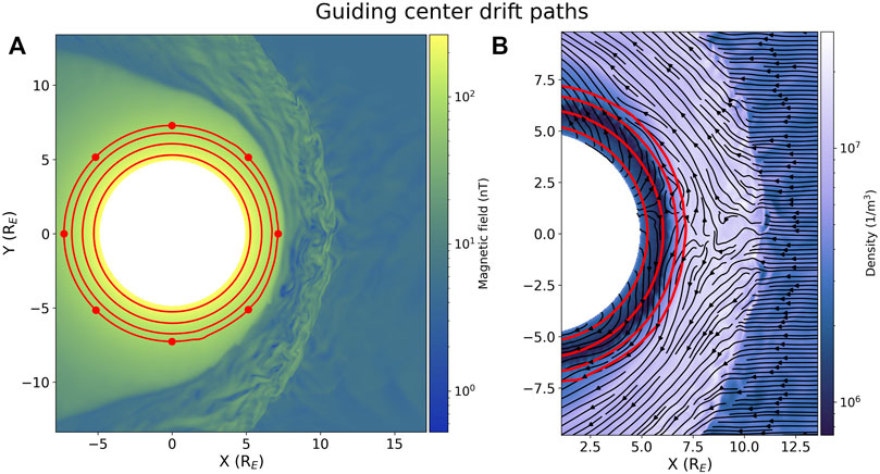
FIGURE 1. Location of the four evaluated guiding center drift paths (red lines) 400 s after the beginning of the simulation. In (A), these are plotted against the total magnetic field and the eight red dots on the outermost drift contour show the locations where the MLT dependent magnetic field time derivatives and L* time derivatives were calculated. In (B), the colour scale shows the plasma density and the black arrows show the velocity streamlines, which can be used to gauge the magnetopause location (Palmroth et al., 2003).
The methodology presented in this paper uses the global electromagnetic field data provided by Vlasiator to calculate the L* time derivative of an electron population without the use of particle tracing. The change in L* over time in the Hamiltonian formalism (Equation A.40 of Lejosne and Kollmann, 2020) is given by
which is valid for equatorial populations in the absence of electrostatic fields. The treatment of the electric field in Vlasiator, with Faraday’s Law correctly resolving the correlation between the induced electric field and time varying magnetic field fluctuations, and the reference frame utilised for the Lagrangian derivative allows for direct evaluation of dL*/dt (and subsequently DL*L*) that includes both the electric and magnetic field fluctuations. This is in contrast to the approach used in, for example, Ozeke et al. (2014); Ali et al. (2016) that separately evaluates the electric and magnetic contributions to the radial diffusion coefficients, which are assumed to be independent and then summed to give the total radial diffusion coefficient.
In this equation, the magnetic field time derivative (dB/dt) and hence dL*/dt are calculated all along the guiding center drift path. The drift averaged magnetic field time derivative, denoted by ⟨⟩φ, is the mean of the local time derivatives. The first adiabatic invariant (μ), drift period (τD) and Lorentz factor (γ) are defined by the population energy, and q is the elementary charge.
The presented methodology involves identifying a guiding center drift path (Section 3.1), determining L* by calculating the magnetic flux through the guiding center drift path (Section 3.2), calculating the magnetic field time derivative at selected magnetic local times (MLT) along this drift path (Section 3.4) and finally calculating dL*/dt for a particle population of a set energy travelling along the guiding center drift path (Section 3.5). The key application of this methodology is the calculation of the radial diffusion coefficients, which we demonstrate in Section 4.
The Vlasiator simulation run used in the methodology development presents some limitations on the populations that can be studied here, namely that the spatially 2D nature limits us to equatorial particles and that the drift period of the population must be less than the simulation duration. We therefore study ultrarelativistic equatorial populations with drift orbits in the outer radiation belt within the simulation domain, and present the L* time derivatives and preliminary radial diffusion coefficients for these populations.
The guiding center drift paths of electron populations were identified directly from magnetospheric magnetic field isocontours. Test particle tracing is an alternative approach for the identification of drift paths from simulations (as in e.g., Huang et al., 2010). The use of magnetic field isocontours for drift path identification is independent of electron energy as multiple different electron populations can drift along the same isocontour, while other test particle tracing only evaluate populations of specified energy or adiabatic invariants. As a bonus, drift path identification from magnetic field isocontours is significantly less computationally expensive than test particle tracing.
Four guiding center drift paths are presented in this manuscript to demonstrate the methodology. They correspond to the 210 nT, 140 nT, 100 nT and 80 nT magnetic field isocontours of the total magnetic field provided by Vlasiator, which were selected to be approximately evenly spaced throughout the outer radiation belt. The four isocontours remained closed loops centered on the Earth throughout the simulation and therefore represent the guiding center drift paths of trapped radiation belt populations, although care must be taken to remain sufficiently far from the magnetopause so that the gyromotion of the particle does not result in magnetopause shadowing. These drift paths correspond to L-shells of 5.28, 6.04, 6.75 and 7.27 respectively, as calculated from the median radial distance of the magnetic field isocontour averaged over time from 350 s after the beginning of the simulation until its end. The assumption that the guiding center drift path can be modelled by the magnetic isocontour holds for slowly varying magnetic fields (fluctuating on timescales significantly greater than the bounce period), so we additionally take a 10 s running average of the isocontour location to ensure that there are no rapid changes that would violate this assumption. We refer to the 10 s average of the drift path throughout the remainder of the study, not the instantaneous drift path, unless otherwise specified.
Figure 1 shows the locations of these magnetic field isocontours within the magnetosphere. Subplot 1a shows the complete drift paths within the outer radiation belt against the total magnetic field, while subplot 1b shows these in relation to the dayside plasma flow. The magnetopause location can be gauged in subplot b at locations where the streamlines diverge around the obstacle (Palmroth et al., 2003). The three innermost drift paths are firmly within the magnetosphere, as seen by the lower density region. The outermost drift path borders a region of significantly higher density and there is some sunwards plasma flow across this drift path. This means that this drift path borders the edge of the magnetosphere, skimming the boundary of the outer radiation belt environment. The 80 nT isocontour therefore represents the most distant drift path that can be studied in this simulation using this approximation. The inner boundary at 5 RE additionally restricts the range of drift path locations that can be studied in this simulation. The 210 nT isocontour, located at L-shell of 5.28, represents the innermost drift path that can be studied here, although there is still the possibility of boundary effects at this location due to the close proximity to the inner boundary. Therefore, this selection of magnetic isocontours represents the full spatial range of guiding center drift paths that could be represented in this simulation.
The average radial distance of each drift path is shown as a function of MLT in Figure 2. This was obtained by calculating the median radial distance of the instantaneous drift path in 2 min MLT bins at a given timestep of the simulation, and then taking the average value in each MLT bin throughout the simulation to obtain the time-averaged radial distance. We observe that the guiding center drift path is more distant on the dayside of the Earth than the nightside, which is due to the dayside compression and nightside stretching of the Earth’s magnetic field. The drift paths at the lowest three L-shells have a sinusoidal relationship between radial distance and magnetic local time, although the drift path represented by the 100 nT isocontour is slightly distorted from the sinusoidal relation and we see a slight asymmetry between the pre-noon and post-noon distribution. This configuration of the magnetic field isocontours is consistent with the Mead magnetospheric model, which predicts a sinusoidal relationship between radial distance and MLT along a magnetic field isocontour (Mead and Fairfield, 1975). The relationship between radial distance and MLT significantly differs at the most distant drift path (L = 7.27). Along this drift path, there is a sinusoidal relationship between radial distance and MLT until approximately local noon, after which the radial distance begins to significantly decrease. There is a significant compression of the drift path throughout the afternoon sector until dusk, when recovery begins and the drift path returns to a more distant radial location. This indicates a persistent magnetic field distortion in the afternoon sector, likely due to the asymmetric interplanetary magnetic field causing greater buildup on the dusk flank and thus compressing the magnetopause closer to the Earth in this sector. The distribution of the most distant isocontour is therefore inconsistent with the Mead model. However, as discussed earlier, this magnetic field isocontour may pass beyond the magnetopause, in which case the sinusoidal relationship between L and MLT predicted in the Mead model would not apply.
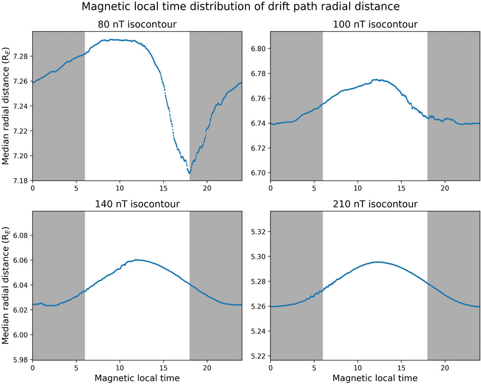
FIGURE 2. Radial distance of each guiding center drift path as a function of magnetic local time. This is taken from the median radial distance binned in 2 minute MLT bins, which is then averaged from 350 s after the beginning of the simulation until its end. The y-range is the same in each subplot but the absolute values are different. The white and grey shading represent magnetic local times corresponding to day and night respectively.
The third adiabatic invariant of a population is proportional to the magnetic flux through the surface bounded by the guiding center drift path, or equivalently the Roederer L* coordinate. Traditionally, the magnetic flux is calculated by tracing the magnetic field lines at the drift path back to the Earth’s surface and then calculating the flux through that area (Roederer, 1970; Min et al., 2013; Lejosne, 2014; Roederer and Lejosne, 2018), but this approach was not possible in this simulation due to its spatially 2D nature. We instead use an equivalent method where the magnetic flux through the drift path is calculated by summing the flux contributions of the dipole magnetic field and the deviation from the dipolar field (perturbed magnetic field, δB) provided by Vlasiator. The perturbed magnetic field was assumed to be zero within the inner boundary, i.e. that there was a purely dipolar magnetic field at r < 5 RE. The Earth’s magnetic field is approximately dipolar below 4 RE (Roederer and Zhang, 2014), so it is reasonable in the quiet radiation belt environment of this simulation to take a dipole magnetic field to 5RE and then include non-dipole magnetic field perturbations beyond this point. The dipole flux (ΦD) is calculated according to
where R was taken to be the median radial distance of the magnetic field isocontour over MLT at time t. The perturbed flux (ΦP) is calculated from the sum of the perturbed flux in the z direction in a given cell multiplied by the cell surface area (cA). We therefore define the perturbed flux as
where n is the number of cells within the drift path at a given time and δBz(t) is the z component of the perturbed magnetic field of a given cell. The total flux through the surface bounded by the magnetic field isocontour at a given time is therefore calculated as
allowing for direct calculation of the time variation of the third adiabatic invariant from the geomagnetic field. Figure 3 shows the fluxes through each of the four magnetic field isocontours as a function of time and the corresponding Roederer L* coordinates. Table 1 compares the L-shell and time-averaged L* coordinates calculated at each drift path. In each case, the variation along L* of a drift path is slightly smaller than the corresponding L-shell value (on the order of 10−2–10−1), with increasing difference between L* and L-shell with increasing radial distance, which is explained by the radiation belt conditions in this simulation that result in low levels of magnetic field distortion from the dipole configuration.
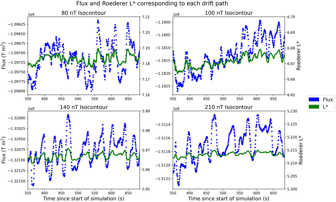
FIGURE 3. Magnetic fluxes through each of the guiding center drift paths as a function of time. The Roederer L* of a trapped population drifting along each path is calculated from the flux value at a given time. The magnetic flux corresponds to the left axis of each subplot while the right axis corresponds to the L* coordinate.
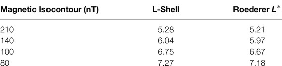
TABLE 1. L-shell and Roederer L* coordinates for the four guiding center drift paths. The L-shell and L* values are averaged over time and are given to three significant figures.
Magnetospheric wave activity in the simulation used in this study was generated primarily by foreshock waves that were transferred to the magnetosphere. Palmroth et al. (2015) found that this simulation produces compressive 30 s ULF waves in the foreshock, while Takahashi et al. (2021) found that a Vlasiator run with different solar wind conditions resulted in transmission of foreshock waves to the magnetosphere. This simulation was run with fixed solar wind parameters, so there were no variations in the solar wind that could drive magnetospheric ULF activity (as observed in e.g. Agapitov and Cheremnykh, 2013), while the geometry of the simulation meant that there was no substorm activity, which is another possible source of ULF waves (e.g. Zolotukhina et al., 2008). Therefore, transmission of foreshock generated waves across the magnetopause was the dominant source of ULF wave activity in this simulation. Foreshock waves in the simulation used in this study are predominantly in the 30–40 s range, although they are also observed at periods ranging from 15 – 55 s (Palmroth et al., 2015; Turc et al., 2018), so they encompass almost the full ULF Pc3 range and some ULF Pc4 wave activity. Takahashi et al. (2021) found that the amplitude of foreshock transmitted waves was dependent on both MLT and L-shell, with highest amplitude closest to the magnetopause and significant amplitude difference between the dayside and nightside. This damping of waves as they enter the magnetosphere would therefore translate to weaker radial diffusion in the inner magnetosphere than would occur with more driving wave activity.
We used the Morlet wavelet transform (Torrence and Compo, 1998) of the perturbed magnetic field to evaluate the wave activity present in the outer radiation belt during this simulation. We took the magnetic field data from eight equally spaced points along each drift path, which are at 3 h MLT intervals and are represented by the red dots in Figure 1A. A spectrogram of the wave activity at local noon of each drift path is shown in Figure 4, subplots a–d, as an example of the magnetospheric wave activity present in this simulation. The wavelet transform was applied to the z component of the perturbed magnetic field, which is representative of the compressional wave activity. Compressional waves are the only waves that are well represented in this simulation due to its 2D nature, as the coupling of magnetospheric fast mode waves to magnetic field line resonances require 3D treatment (see Takahashi et al., 2021, for further discussion), so these spectrograms are representative of the wave activity driving radial diffusion in this simulation. In these subplots, the wave power is represented by the colour scale, the 95% confidence interval for background wave activity (calculated according to Torrence and Compo, 1998) is shown by solid black lines, the cone of influence (COI) is represented by the black mesh and the dashed red lines show the boundaries between the ULF Pc ranges. The COI is the region of the wavelet spectrum that experiences time-domain boundary effects and is determined by the duration of the time period that the wavelet analysis is performed over, with shorter durations resulting a larger proportion of wave activity within the COI. Subplot 4E shows how long each wave period exists outside the cone of influence. Here the duration of wavelet analysis is limited by the duration of the simulation, which is such that all Pc5 activity is within the COI and Pc4 wave activity is only outside the COI for a small portion of the simulation run time. The duration of the evaluated portion of the simulation is 335 s, so waves with period
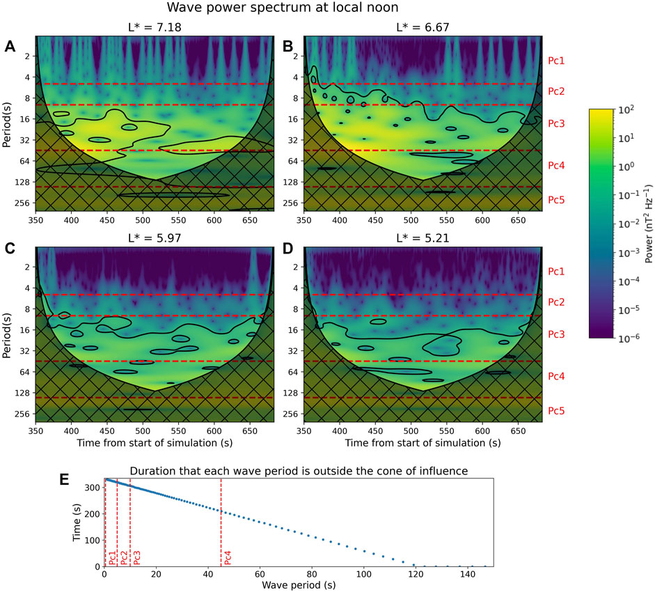
FIGURE 4. Subplots (A-D) show the wavelet power spectra calculated from the Morlet transform of perturbed magnetic field at noon on each drift path evaluated in this study. The solid black lines represent the 95% confidence interval and the black mesh shows the cone of influence in these subplots. Subplot (E) shows the duration that the wave of a given period is present in the simulation for, i.e. how long the wave is outside the cone of influence. Red dashed lines mark the periods dividing the ULF Pc ranges in each subplot.
The 95% confidence intervals indicate significant wave activity. We observe from Figure 4 that the majority of significant wave activity occurs in the Pc3 range, although there is some significant Pc2 activity. ULF Pc4 waves are also significant when they are outside the COI, although only a small proportion of these waves are present in the simulation for long enough to complete multiple cycles. There is no significant Pc1 activity, although we observe some broadband structures in the Pc1 range, particularly at the most distant drift path. The primary effect of the 10 s smoothing of the drift path location was the averaging out of some of these broadband structures, with longer period wave activity remaining unaffected. The extremely low levels of Pc1 activity (note the logarithmic scale in Subplot 4A–D) means that none of the dL*/dt analysis (presented later in Section 4) is affected by the removal of some Pc1 waves. Therefore, the Pc3 wave activity dominates for the majority of the simulation run time, with additional significant Pc4 activity for a small portion of the simulation, so the changes in L* studied here are primarily driven by ULF Pc3 wave activity. In the Earth’s magnetosphere, changes in L* are primarily due to ULF Pc5 activity, as these waves are able to cause drift-resonant diffusion of outer radiation belt populations (e.g Su et al., 2015). We here use the Pc3-dominated simulation to develop the methodology to calculate dL*/dt, which can be then applied to longer duration simulations that include the longer period waves that drive drift-resonant radial diffusion.
We then calculated the power spectral density (PSD) of the magnetic field perturbations at each MLT point along the four drift paths, excluding all data within the COI. Figure 5 shows the distribution of the mean PSD in each ULF Pc range over MLT and L*. We observe that the PSD is generally higher on the dayside than the nightside, with peak PSD occurring at or near local noon, and increasing mean PSD with increasing L*. Both of these trends are consistent with the L-shell and MLT distribution of foreshock transmitted ULF waves discussed earlier. The Pc4 PSD, however, peaks at MLT 03 at the lowest L*, which is most likely an inner boundary effect as this spatial distribution is highly inconsistent with foreshock transmitted waves. This peak occurs at period 87.2 s, which is resolved in the simulation for 94 s and so completes only one full cycle. We emphasize however that the masking of wave activity inside the COI means that the Pc4 waves are only present for a small portion of the simulation, so this unphysical peak likely does not persist for long enough to affect the rest of the analysis.
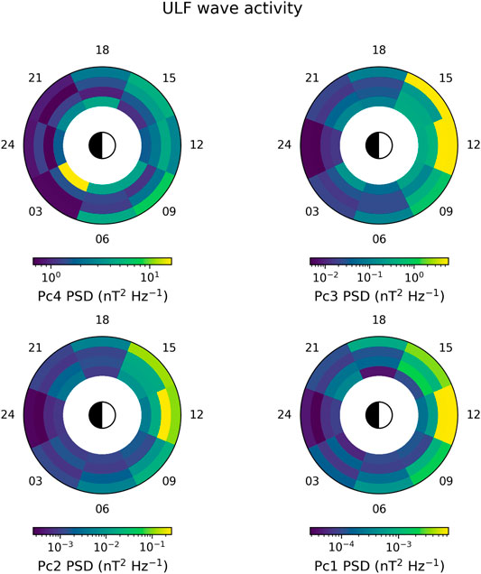
FIGURE 5. L*-MLT maps of the mean power spectral density in each ULF Pc range, as calculated from the Morlet transform of the z component of the perturbed magnetic field, excluding data inside the cone of influence. The ULF Pc5 PSD is not shown as these periods are inside the COI throughout the simulation. The MLT value is shown by the angular location of the bins, while the four radial bins represent the four drift paths. Note that the radial distances are not to scale and that the colour scale varies between subplots.
Figure 6 shows the PSD distribution as a function of wave period along each drift path. The Pc1 and Pc2 PSD is low at all periods, L* and MLT, while significant activity occurs in the Pc3 and Pc4 ranges. At MLT of 12 and 15, we observe peaks in the PSD at periods of approximately 20 and 40 s along the outer drift paths. There are larger peaks in the Pc4 range at periods of ∼ 100 s, but, as waves at these periods are only outside the COI for a short time, the Pc3 waves are the primary driver of L* fluctuations for the majority of this simulation, with Pc4 waves only driving L* fluctuations for a small portion of the simulation.

FIGURE 6. Power spectral density along the four evaluated drift paths at each evaluated magnetic local time. The PSD was calculated according to the Morlet transform of the z component of the perturbed magnetic field, and all data inside the cone of influence were excluded. The x-axes are set such that only waves that are present in the simulation for more than two cycles are shown. All subplots are shown with the same y-axes to aid comparison between MLT; peak PSD at MLT = 3 and L* = 5.21 reached 52.3 nT2 Hz−1 at period 87.2 s, which is most likely a boundary artifact.
The magnetic field time derivative was calculated at the same eight points along the drift paths as in the wave analysis, which are shown in Figure 1A. The Lagrangian derivative was used in order to include the effects of the electric field on magnetic field fluctuations, following the approach outlined in Section 4 of Lejosne (2019). This was obtained using the total time derivative
where v is the velocity of the guiding center resulting from the electric and magnetic drifts
Here, v⊥ is the initial velocity perpendicular to the magnetic field, q is the particle charge and m is the particle mass. Since the magnetic drift is perpendicular to the magnetic field gradient, the total magnetic field time derivative is
We approximate the partial magnetic field time derivative as
where N is the number of MLT points along the drift path. The magnetic and electric field data were processed in order to exclude the contributions of wave activity inside the cone of influence. As in Section 3.3, this was done by calculating the Morlet transform of the perturbed magnetic field and total electric field, masking all data inside the cone of influence, and then reconstructing the magnetic or electric field time series according to Eq. (11) of Torrence and Compo (1998). The background dipolar magnetic field from Vlasiator was then added to the reconstructed perturbed magnetic field data. This provided magnetic and electric field data with fluctuations solely caused by waves that were resolved in the simulation. The number of MLT points that need to be evaluated to properly represent the driving wave activity is contingent on the distribution of wave activity in MLT. If a simulation generated wave activity that is significantly enhanced in, for example, the dusk sector while remaining at a low level in other sectors, a significantly greater number of MLT points would be needed to correctly evaluate the wave activity that a particle experiences over its drift. Conversely, in a simulation without highly localised wave activity, such as the one used in the development of this methodology, the total wave activity over a drift orbit can be described by a lower number of MLT points. We examine the wave activity, dB/dt and dL*/dt at eight MLT points (shown in Figure 1) here to develop and demonstrate the methodology; full analysis of the effect of N on the drift averaged magnetic field derivative and subsequent impact on the radial diffusion coefficients will be evaluated in a future study.
Figure 7 shows the local magnetic field time derivative at different MLT along each drift path. The nightside magnetic field fluctuations were extremely low, with significant dB/dt first arising at dawn (MLT = 6) and fading at dusk (MLT = 18). Greatest magnetic field fluctuations occurred at MLT of 12 and 15, and dB/dt at MLT = 9 was also elevated from the dawn and dusk values. The strong Pc3 activity observed at MLT of 12 and 15 was responsible for the elevated dB/dt at these locations. However, visual inspection of this figure additionally reveals some fluctuations in the low-period Pc4 range (
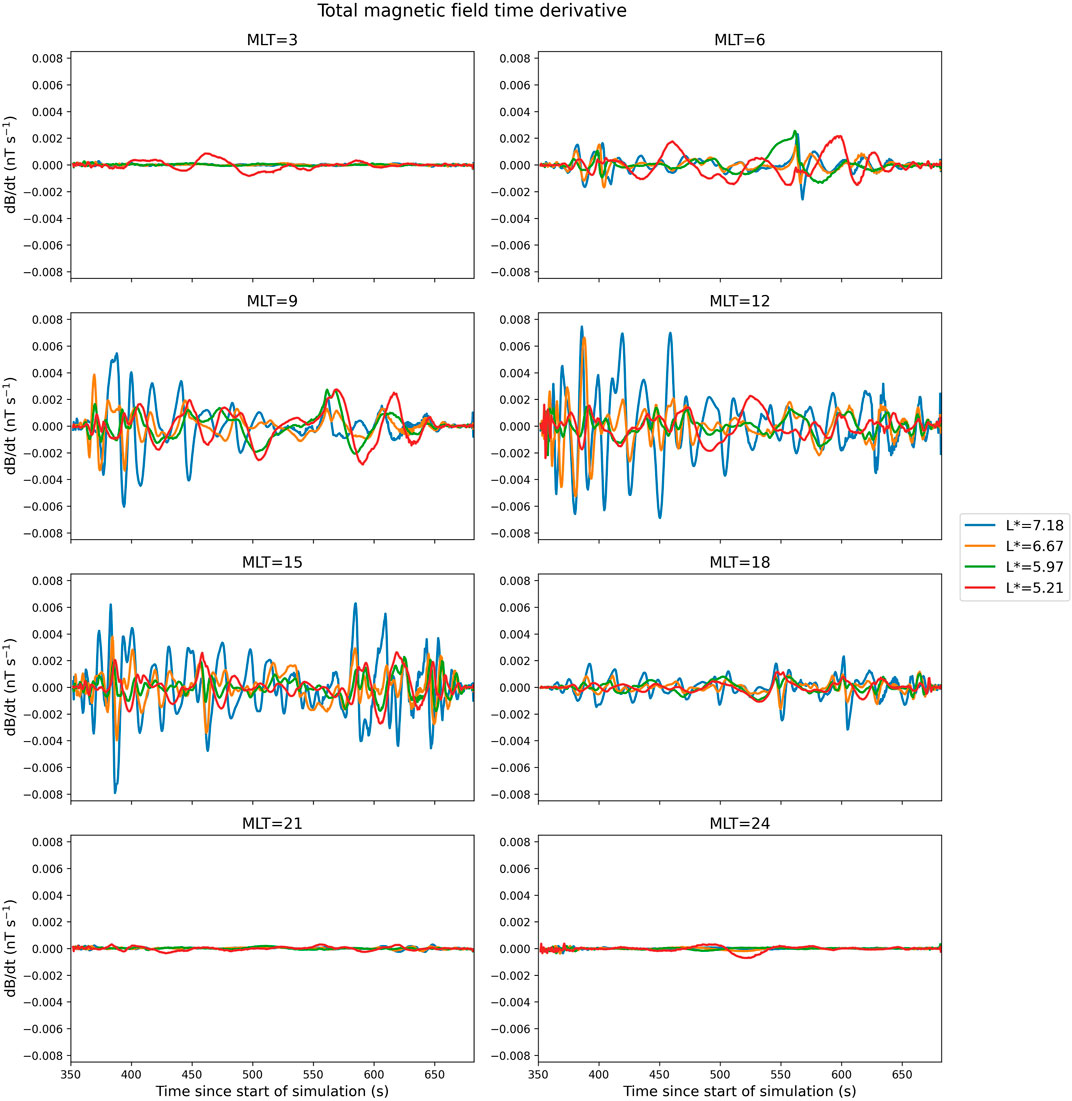
FIGURE 7. Local magnetic field time derivative at selected magnetic local times along each drift path, excluding contributions from wave activity within the cone of influence.
The drift-averaged magnetic field time derivatives are shown in Figure 8 for the four selected drift paths. The amplitude of the drift-averaged fluctuations increases with increasing L*, which is again consistent with wave activity due to foreshock-transmitted ULF waves. The majority of the fluctuations along each drift contour are in the Pc3 range, although some fluctuations occur at Pc4 periods for a short portion of the simulation, as shown by visual inspection of the figure. Fluctuations in the Pc1 and Pc2 range occur briefly at the start and end of the evaluated time period for each drift path, but this is due to all other wave activity being inside the COI at these times and therefore being excluded from the magnetic field time derivative calculations. The Pc1 and Pc2 fluctuations at these times are at significantly lower amplitudes than the longer period waves, so the drift-averaged driving is primarily again due to Pc3 wave activity.
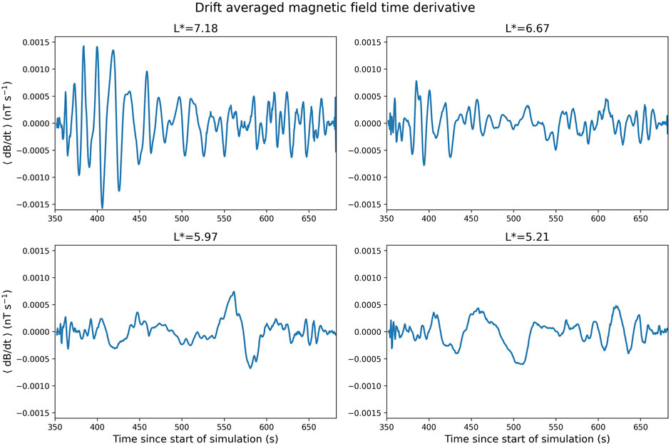
FIGURE 8. Drift averaged magnetic field time derivative along each drift path as a function of time. These are calculated from the mean of the local magnetic field time derivatives and are driven by foreshock transmitted ULF waves.
The magnetic fluxes and fluctuations obtained from Vlasiator were then used to calculate the L* time derivative for outer radiation belt electron populations travelling along the four investigated guiding center drift paths (Figure 1). The calculation of L* time derivative also requires the first adiabatic invariant (μ), drift period
In these equations, Ekin is the kinetic energy of the electron population, B is the magnetic field strength along the drift path and L is L-shell. The constant terms are electron rest energy (E0), electron charge (q), equatorial magnetic field (BE) and Earth radius (RE). The equation for Ω assumes a dipolar magnetic field, which is a valid approximation for equatorial particles sampling the geomagnetic field sustained in this simulation. Using this approach, we can evaluate the dL*/dt of any equatorial population travelling along a given drift path as long as the corresponding drift period is significantly less than the simulation duration.
We first evaluated dL*/dt using Eq. (5) for ultrarelativistic electron populations with energies of 3 MeV, examining only equatorial populations due to the spatially 2D simulation, studying the same four guiding center drift paths. Table 2 shows the population specific quantities corresponding to this energy at each drift path. We additionally note that the gyroperiod is on the order of 1–3 ms, bounce period is 0.3–0.4 s and drift period is 4–5 min for this population at L-shell of 5–7 under the dipole approximation, so the 10 s averaging of the drift path discussed in Section 3.1 is indeed between the bounce and drift period.
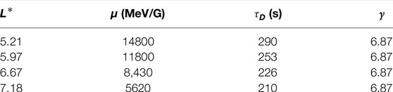
TABLE 2. Key variables for a 3 MeV electron population travelling along the selected drift paths that were used in the calculation of the L* time derivative. These values are given to three significant figures.
The time derivative of L* of the 3 MeV population at each evaluated magnetic local time along the four drift paths is shown in Figure 9. The behaviour of dL*/dt closely followed the magnetic field time derivative shown in Figure 7, as was expected, and predominantly varied at periods corresponding to the ULF Pc3 waves. There was a clear increase in dL*/dt amplitude with increasing L*, so greatest fluctuations occurred along the drift path closest to the magnetopause. There was also a significant dependence of dL*/dt on magnetic local time, with significantly greater fluctuations on the dayside than on the nightside. At the innermost three drift contours, greatest amplitude dL*/dt occurred at MLT of 12, while similarly high amplitudes occurred at MLT of 12 and 15 on the outermost drift path. The greatest dL*/dt occurred at the MLT points along each drift path where ULF Pc3 wave activity was strongest. We did not observe significant dL*/dt fluctuations at MLT = 03 on the innermost drift contour, where the large peak in ULF Pc4 wave activity occurred due to inner boundary effects. This is most likely because subtracting the local magnetic time derivative from the drift averaged derivative smoothed out the contribution of this highly localised peak. The Pc1 and Pc2 wave activity was too low at all MLTs and drift paths to violate the third adiabatic invariant, and thus, did not have significant contribution to dL*/dt. Therefore, the primary drivers of the observed variations in L* in this simulation were ULF Pc3 waves that were generated in the foreshock and transmitted to the inner magnetosphere.
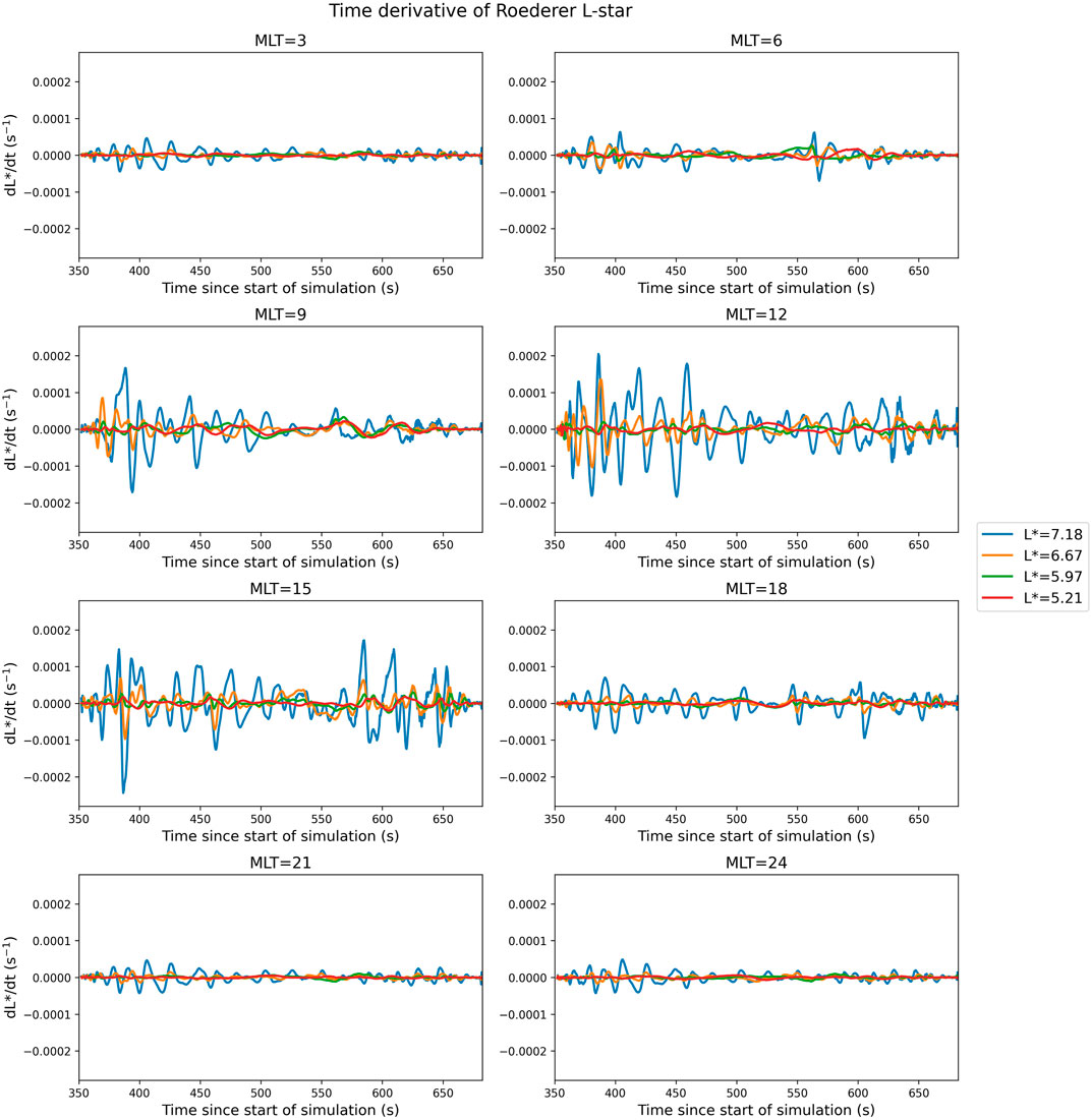
FIGURE 9. L* time derivative of a 3 MeV equatorial electron population along the four evaluated drift paths in the outer radiation belt. Changes in L* are here primarily driven by ULF Pc3 wave activity that is transmitted from the foreshock to the magnetosphere.
In order to test the key application of this methodology, we calculated the radial diffusion coefficients of a 3 MeV electron population travelling along the four drift paths. The radial diffusion coefficient is defined in terms of change in L* (Eq. (4)), which we approximate as
taking a timestep of Δt = 1 s. The DL*L* results are 1.25 × 10⁻⁶ day−1, 2.01 × 10⁻⁶ day−1, 1.0 × 10⁻⁵ day−1 and 5.68 × 10⁻⁵ day−1, in order of increasing L*. While these values are significantly lower than those reported in the literature (e.g., the Ozeke et al., 2014, model gives values on the order of 10−3–10−2 day−1 for KP = 0 at these locations), they are reasonable given the radiation belt environment and low wave activity present in the simulation. The obtained values of DL*L* increase with increasing L*;, as is expected, although further conclusions on the relationship between DL*L* and L* obtained with this methodology can not be drawn with only four data points.
A radial diffusion study using an alternative methodology was performed by Huang et al. (2010), who evaluated the radial diffusion coefficients of relativistic equatorial electrons using test particle tracing in combination with a global MHD code. The simulation with driving solar wind speed Vx = 400 km s−1 produced a mean wave amplitude of 1 nT at geosynchronous orbit and results in DL*L* on the order of 10–4 − 10–3 over the same L* range as evaluated in this study. We note that wave activity in Huang et al. (2010) had greatest PSD in the ULF Pc5 range and that these waves were primarily generated by periodic dynamic pressure variations in the driving solar wind, as opposed to the foreshock-transmitted waves present in the simulation evaluated in this study. We have driving wave activity that is of significantly lower amplitude and is in a frequency range that does not cause drift-resonant radial diffusion, so it is consistent that the DL*L* obtained in this study are approximately two orders of magnitude lower than those presented in Huang et al. (2010) at a given L*. We expect that when this methodology is applied to a simulation with both higher amplitude wave activity and wave activity in the ULF Pc4 and Pc5 range, the resulting DL*L* values will be more in line with those reported previously in the literature. Therefore, the methodology presented in this paper produces physically reasonable results for the radial diffusion coefficients in a non-dipolar geomagnetic field. Application of this methodology to simulations that provide the global magnetic field topology in near-Earth space offers a novel technique to calculate the L* time derivative and radial diffusion coefficients that provides an alternative to the test particle tracing approach.
In this study, we presented a novel methodology that uses global electric and magnetic field data provided by Vlasiator, a hybrid-Vlasov simulation of near-Earth space, to calculate the time derivative of the Roederer L* coordinate (dL*/dt) for an outer radiation belt electron population. While this methodology can also be applied to magnetohydrodynamic simulations, hybrid-Vlasov simulations give a more complete view of the magnetospheric magnetic field due to the ion-hybrid approach. This methodology uses the global field data from the Vlasiator simulation to calculate the third adiabatic invariant of a population and local and drift-averaged wave activity driving radial diffusion, in combination with population specific variables calculated from the energy of the population, to determine the more fundamental dL*/dt without the use of test particle tracing. We applied this methodology to provide a first approximation to the radial diffusion coefficients from dL*/dt for equatorial, ultrarelativistic electron population.
We developed this methodology using a simulation in the equatorial plane with a constant driving solar wind, in which radiation belt wave activity is primarily due to ULF waves that were generated in the foreshock and transmitted to the magnetosphere. This wave activity is low amplitude with most significant activity in the ULF Pc3 range, but the magnetic local time asymmetry of the ULF waves still drives radial diffusion and causes changes in L*. When accounting for these magnetospheric conditions, the radial diffusion coefficients calculated from dL*/dt obtained using this methodology are physically reasonable, although they are significantly lower than other radial diffusion coefficients reported in the literature that include ULF Pc4 and Pc5 waves and often evaluate a more active radiation belt environment.
The presented methodology to calculate the L* time derivative and its application to the calculation of the radial diffusion coefficients presents multiple avenues of future research on radial diffusion and the impact of ULF waves on radiation belt dynamics. The methodology can be applied to any simulation that provides global electromagnetic field data, so is suitable for use with both MHD and hybrid simulations. Applying this methodology to a simulation that includes ULF Pc4 and Pc5 wave activity would allow for calculation of dL*/dt and radial diffusion coefficients in a more realistic radiation belt environment. Additional driving of ULF Pc5 wave activity could be achieved with varying solar wind conditions, such as dynamic pressure fluctuations in the Pc5 period range, or substorm activity. This would allow evaluation of the role of specific wave sources to radial diffusion in the outer radiation belt. Additionally, the wave masking could be used to investigate the effect of different ULF Pc wave ranges separately. This would reveal the impact of different ULF period ranges on radial diffusion, which is otherwise difficult to achieve as the effects of lower period waves are hidden by the significantly greater effects of drift-resonant radial diffusion driven by Pc5 waves.
Finally, in addition to presenting new avenues of research into the impact of ULF wave activity on radial diffusion, this methodology allows for rapid comparison of different electron populations undergoing radial diffusion from fundamental properties of radiation belt electrons. A longer simulation would enable evaluation of electron populations at core and relativistic energies in addition to providing ULF Pc5 wave activity, while a spatially 3D simulation would allow for evaluation of non-equatorial populations, allowing for evaluation of the energy and pitch angle dependence of the radial diffusion coefficients. Therefore, as new advances are made with global simulations, the methodology outlined in this study presents new opportunities for studies on the impact of ULF waves on outer radiation belt electron populations.
Publicly available datasets were analyzed in this study. This data can be found here: http://github.com/fmihpc/vlasiator.
HG carried out the analysis and wrote the paper under the supervision of AO and EK. AO and SL assisted in theoretical understanding of radial diffusion. LT assisted with wave analysis and interpretation. UG and YP-K have made significant contributions to the simulation methods and analysis. All co-authors helped in the interpretation and visualization of the results, and read and commented on the paper.
We acknowledge The European Research Council for starting grant 200141-QuESpace, with which Vlasiator (http://helsinki.fi/vlasiator) was developed, and Consolidator grant 682068-PRESTISSIMO awarded to further develop Vlasiator and use it for scientific investigations. We gratefully also acknowledge the Finnish Center of Excellence in Research of Sustainable Space (Academy of Finland grant number 312351), and Academy of Finland grant numbers 338629, 339756, 309937, and 328893. The CSC - IT center for Science in Finland and the PRACE Tier-0 supercomputer infrastructure in HLRS/Stuttgart (grant numbers PRACE-2012061111 and PRACE-2014112573) are acknowledged as they made these results possible. EK acknowledges the European Research Council (ERC) under the European Union’s Horizon 2020 Research and Innovation Programme Project SolMAG 724391, and Academy of Finland project 310445. LT acknowledges the Academy of Finland grant 322544 and the University of Helsinki (3-year research grant 2020-2022). SL work was performed under NASA Grant Award 80NSSC18K122.
The authors declare that the research was conducted in the absence of any commercial or financial relationships that could be construed as a potential conflict of interest.
All claims expressed in this article are solely those of the authors and do not necessarily represent those of their affiliated organizations, or those of the publisher, the editors and the reviewers. Any product that may be evaluated in this article, or claim that may be made by its manufacturer, is not guaranteed or endorsed by the publisher.
We gratefully acknowledge The European Research Council, the Finnish Center of Excellence in Research of Sustainable Space and the Academy of Finland for their funding.
Agapitov, O., and Cheremnykh, O. (2013). Magnetospheric ULF Waves Driven by External Sources. Adv. Astron. Space Phys. 3, 12–19.
Ali, A. F., Malaspina, D. M., Elkington, S. R., Jaynes, A. N., Chan, A. A., Wygant, J., et al. (2016). Electric and Magnetic Radial Diffusion Coefficients Using the Van Allen Probes Data. J. Geophys. Res. Space Phys. 121, 9586–9607. doi:10.1002/2016JA023002
Anderson, B. J. (1994). “An Overview of Spacecraft Observations of 10 S to 600 S Period Magnetic Pulsations in the Earth’s Magnetosphere,” in Washington DC American Geophysical Union Geophysical Monograph Series. Washington: DC by American Geophysical Union, 81, 25–43. doi:10.1029/GM081p0025
Battarbee, M., Hannuksela, O. A., Pfau-Kempf, Y., von Alfthan, S., Ganse, U., Jarvinen, R., et al. (2021). Fmihpc/Analysator: v0.9. doi:10.5281/zenodo.4462515
Brautigam, D. H., and Albert, J. M. (2000). Radial Diffusion Analysis of Outer Radiation belt Electrons during the October 9, 1990, Magnetic Storm. J. Geophys. Res. 105, 291–309. doi:10.1029/1999JA90034410.1029/1999ja900344
Brautigam, D. H., Ginet, G. P., Albert, J. M., Wygant, J. R., Rowland, D. E., Ling, A., et al. (2005). CRRES Electric Field Power Spectra and Radial Diffusion Coefficients. J. Geophys. Res. 110. doi:10.1029/2004JA010612
Cunningham, G. S. (2016). Radial Diffusion of Radiation belt Particles in Nondipolar Magnetic fields. J. Geophys. Res. Space Phys. 121, 5149–5171. doi:10.1002/2015JA021981
Dai, L., Takahashi, K., Lysak, R., Wang, C., Wygant, J. R., Kletzing, C., et al. (2015). Storm Time Occurrence and Spatial Distribution of Pc4 Poloidal Ulf Waves in the Inner Magnetosphere: A Van allen Probes Statistical Study. J. Geophys. Res. Space Phys. 120, 4748–4762. doi:10.1002/2015JA021134
Davis, L. , and Chang, D. B. (1962). On the Effect of Geomagnetic Fluctuations on Trapped Particles. J. Geophys. Res. 67, 2169–2179. doi:10.1029/JZ067i006p02169
Dorelli, J. C., Glocer, A., Collinson, G., and Tóth, G. (2015). The Role of the Hall Effect in the Global Structure and Dynamics of Planetary Magnetospheres: Ganymede as a Case Study. J. Geophys. Res. Space Phys. 120, 5377–5392. doi:10.1002/2014JA020951
Dreher, J., and Schindler, K. (1997). Three-dimensional Hall-Mhd Simulations of Magnetopause Reconnection. Phys. Chem. Earth 22, 747–750. doi:10.1016/S0079-1946(97)00206-1
Elkington, S. R., Hudson, M. K., Wiltberger, M. J., and Lyon, J. G. (2002). MHD/particle Simulations of Radiation belt Dynamics. J. Atmos. Solar-Terrestrial Phys. 64, 607–615. doi:10.1016/S1364-6826(02)00018-4
Fälthammar, C.-G. (1965). Effects of Time-dependent Electric fields on Geomagnetically Trapped Radiation. J. Geophys. Res. 70, 2503–2516. doi:10.1029/JZ070i011p02503
Huang, C.-L., Spence, H. E., Hudson, M. K., and Elkington, S. R. (2010). Modeling Radiation belt Radial Diffusion in ULF Wave fields: 2. Estimating Rates of Radial Diffusion Using Combined MHD and Particle Codes. J. Geophys. Res. 115, n/a. doi:10.1029/2009JA014918
Jacobs, J. A., Kato, Y., Matsushita, S., and Troitskaya, V. A. (1964). Classification of Geomagnetic Micropulsations. J. Geophys. Res. 69, 180–181. doi:10.1029/JZ069i001p00180
Kennel, C. F., and Petschek, H. E. (1966). Limit on Stably Trapped Particle Fluxes. J. Geophys. Res. 71, 1–28. doi:10.1029/JZ071i001p00001
Kokubun, S., Erickson, K. N., Fritz, T. A., and McPherron, R. L. (1989). Local Time Asymmetry of Pc 4-5 Pulsations and Associated Particle Modulations at Synchronous Orbit. J. Geophys. Res. 94, 6607–6625. doi:10.1029/JA094iA06p06607
Lejosne, S. (2014). An Algorithm for Approximating the L * Invariant Coordinate from the Real-Time Tracing of One Magnetic Field Line between Mirror Points. J. Geophys. Res. Space Phys. 119, 6405–6416. doi:10.1002/2014ja020016
Lejosne, S. (2019). Analytic Expressions for Radial Diffusion. J. Geophys. Res. Space Phys. 124, 4278–4294. doi:10.1029/2019JA026786
Lejosne, S., and Kollmann, P. (2020). Radiation belt Radial Diffusion at Earth and beyond. Space Sci. Rev. 216. doi:10.1007/s11214-020-0642-6
Li, Z., Hudson, M., Patel, M., Wiltberger, M., Boyd, A., and Turner, D. (2017). ULF Wave Analysis and Radial Diffusion Calculation Using a Global MHD Model for the 17 March 2013 and 2015 Storms. J. Geophys. Res. Space Phys. 122, 7353–7363. doi:10.1002/2016JA023846
McIlwain, C. E. (1961). Coordinates for Mapping the Distribution of Magnetically Trapped Particles. J. Geophys. Res. 66, 3681–3691. doi:10.1029/JZ066i011p03681
Mead, G. D., and Fairfield, D. H. (1975). A Quantitative Magnetospheric Model Derived from Spacecraft Magnetometer Data. J. Geophys. Res. 80, 523–534. doi:10.1029/JA080i004p00523
Min, K., Bortnik, J., and Lee, J. (2013). A Novel Technique for rapidL*calculation Using UBK Coordinates. J. Geophys. Res. Space Phys. 118, 192–197. doi:10.1029/2012JA018177
Northrop, T. G. (1963). Adiabatic Charged-Particle Motion. Rev. Geophys. 1, 283–304. doi:10.1029/rg001i003p00283
Nosé, M., Iyemori, T., Nakabe, S., Nagai, T., Matsumoto, H., and Goka, T. (1998). ULF Pulsations Observed by the ETS-VI Satellite: Substorm Associated Azimuthal Pc 4 Pulsations on the Nightside. Earth Planet. Sp 50, 63–80. doi:10.1186/BF03352087
Olifer, L., Mann, I. R., Ozeke, L. G., Rae, I. J., and Morley, S. K. (2019). On the Relative Strength of Electric and Magnetic ULF Wave Radial Diffusion during the March 2015 Geomagnetic Storm. J. Geophys. Res. Space Phys. 124, 2569–2587. doi:10.1029/2018JA026348
Osmane, A., and Lejosne, S. (2021). Radial Diffusion of Planetary Radiation Belts' Particles by Fluctuations with Finite Correlation Time. ApJ 912, 142. doi:10.3847/1538-4357/abf04b
Ozeke, L. G., Mann, I. R., Murphy, K. R., Jonathan Rae, I., and Milling, D. K. (2014). Analytic Expressions for ULF Wave Radiation belt Radial Diffusion Coefficients. J. Geophys. Res. Space Phys. 119, 1587–1605. doi:10.1002/2013JA019204
Ozeke, L. G., Mann, I. R., Murphy, K. R., Rae, I. J., Milling, D. K., Elkington, S. R., et al. (2012). ULF Wave Derived Radiation belt Radial Diffusion Coefficients. J. Geophys. Res. Space Phys. 117, n/a. doi:10.1029/2011ja017463
Palmroth, M., Archer, M., Vainio, R., Hietala, H., Pfau-Kempf, Y., Hoilijoki, S., et al. (2015). ULF Foreshock under Radial IMF: THEMIS Observations and Global Kinetic Simulation Vlasiator Results Compared. J. Geophys. Res. Space Phys. 120, 8782–8798. doi:10.1002/2015JA021526
Palmroth, M., Ganse, U., Pfau-Kempf, Y., Battarbee, M., Turc, L., Brito, T., et al. (2018). Vlasov Methods in Space Physics and Astrophysics. Living Rev. Comput. Astrophys 4. doi:10.1007/s41115-018-0003-2
Palmroth, M., Pulkkinen, T. I., Janhunen, P., and Wu, C.-C. (2003). Stormtime Energy Transfer in Global MHD Simulation. J. Geophys. Res. 108. doi:10.1029/2002JA009446
Parker, E. N. (1960). Geomagnetic Fluctuations and the Form of the Outer Zone of the Van Allen Radiation belt. J. Geophys. Res. 65, 3117–3130. doi:10.1029/JZ065i010p03117
Pfau-Kempf, Y., von Alfthan, S., Sandroos, A., Ganse, U., Koskela, T., Battarbee, M., et al. (2021). Fmihpc/Vlasiator: Vlasiator 5.1. doi:10.5281/zenodo.4719554
Reeves, G. D., Spence, H. E., Henderson, M. G., Morley, S. K., Friedel, R. H. W., Funsten, H. O., et al. (2013). Electron Acceleration in the Heart of the Van Allen Radiation Belts. Science 341, 991–994. doi:10.1126/science.1237743
Roederer, J. G. (1970). Dynamics of Geomagnetically Trapped Radiation. Berlin, Heidelberg: Springer. doi:10.1007/978-3-642-49300-3
Roederer, J. G., and Lejosne, S. (2018). Coordinates for Representing Radiation belt Particle Flux. J. Geophys. Res. Space Phys. 123, 1381–1387. doi:10.1002/2017JA025053
Roederer, J. G. (1967). On the Adiabatic Motion of Energetic Particles in a Model Magnetosphere. J. Geophys. Res. 72, 981–992. doi:10.1029/JZ072i003p00981
Roederer, J. G., and Zhang, H. (2014). Dynamics of Magnetically Trapped Particles. Berlin, Heidelberg: Springer. doi:10.1007/978-3-642-41530-2
Sandhu, J. K., Rae, I. J., Wygant, J. R., Breneman, A. W., Tian, S., Watt, C. E. J., et al. (2021). ULF Wave Driven Radial Diffusion during Geomagnetic Storms: A Statistical Analysis of Van Allen Probes Observations. J. Geophys. Res. Space Phys. 126, e2020JA029024. doi:10.1029/2020JA029024
Schulz, M., and Lanzerotti, L. J. (1974). Particle Diffusion in the Radiation Belts. Berlin: Springer. doi:10.1007/978-3-642-65675-0
Su, Z., Zhu, H., Xiao, F., Zong, Q.-G., Zhou, H., Zheng, Y., et al. (2015). Ultra-low-frequency Wave-Driven Diffusion of Radiation belt Relativistic Electrons. Nat. Commun. 6, 10096. doi:10.1038/ncomms10096
Takahashi, K., Turc, L., Kilpua, E., Takahashi, N., Dimmock, A., Kajdic, P., et al. (2021). Propagation of Ultralow-Frequency Waves from the Ion Foreshock into the Magnetosphere during the Passage of a Magnetic Cloud. J. Geophys. Res. Space Phys. 126, e2020JA028474. doi:10.1029/2020JA028474
Torrence, C., and Compo, G. P. (1998). A Practical Guide to Wavelet Analysis. Bull. Amer. Meteorol. Soc. 79, 61–78. doi:10.1175/1520-0477(1998)079<0061:APGTWA>2.0.CO;2
Turc, L., Ganse, U., Pfau-Kempf, Y., Hoilijoki, S., Battarbee, M., Juusola, L., et al. (2018). Foreshock Properties at Typical and Enhanced Interplanetary Magnetic Field Strengths: Results from Hybrid-Vlasov Simulations. J. Geophys. Res. Space Phys. 123, 5476–5493. doi:10.1029/2018JA025466
von Alfthan, S., Pokhotelov, D., Kempf, Y., Hoilijoki, S., Honkonen, I., Sandroos, A., et al. (2014). Vlasiator: First Global Hybrid-Vlasov Simulations of Earth's Foreshock and Magnetosheath. J. Atmos. Solar-Terrestrial Phys. 120, 24–35. doi:10.1016/j.jastp.2014.08.012
Zhu, X., and Kivelson, M. G. (1991). Compressional ULF Waves in the Outer Magnetosphere: 1. Statistical Study. J. Geophys. Res. 96, 19451–19467. doi:10.1029/91JA01860
Keywords: radial diffusion coefficient, ULF waves, radiation belt, L-star, hybrid-Vlasov simulation, inner magnetosphere
Citation: George H, Osmane A, Kilpua EKJ, Lejosne S, Turc L, Grandin M, Kalliokoski MMH, Hoilijoki S, Ganse U, Alho M, Battarbee M, Bussov M, Dubart M, Johlander A, Manglayev T, Papadakis K, Pfau-Kempf Y, Suni J, Tarvus V, Zhou H and Palmroth M (2022) Estimating Inner Magnetospheric Radial Diffusion Using a Hybrid-Vlasov Simulation. Front. Astron. Space Sci. 9:866455. doi: 10.3389/fspas.2022.866455
Received: 31 January 2022; Accepted: 25 April 2022;
Published: 18 May 2022.
Edited by:
Yoshizumi Miyoshi, Nagoya University, JapanReviewed by:
Scot Elkington, University of Colorado Boulder, United StatesCopyright © 2022 George, Osmane, Kilpua, Lejosne , Turc, Grandin, Kalliokoski, Hoilijoki, Ganse, Alho, Battarbee, Bussov, Dubart, Johlander, Manglayev, Papadakis, Pfau-Kempf, Suni, Tarvus, Zhou and Palmroth. This is an open-access article distributed under the terms of the Creative Commons Attribution License (CC BY). The use, distribution or reproduction in other forums is permitted, provided the original author(s) and the copyright owner(s) are credited and that the original publication in this journal is cited, in accordance with accepted academic practice. No use, distribution or reproduction is permitted which does not comply with these terms.
*Correspondence: H. George, aGFycmlldC5nZW9yZ2VAaGVsc2lua2kuZmk=
Disclaimer: All claims expressed in this article are solely those of the authors and do not necessarily represent those of their affiliated organizations, or those of the publisher, the editors and the reviewers. Any product that may be evaluated in this article or claim that may be made by its manufacturer is not guaranteed or endorsed by the publisher.
Research integrity at Frontiers
Learn more about the work of our research integrity team to safeguard the quality of each article we publish.