Modern Faraday Rotation Studies to Probe the Solar Wind

For decades, observations of Faraday rotation have provided unique insights into the plasma density and magnetic field structure of the solar wind. Faraday rotation (FR) is the rotation of the plane of polarization when linearly polarized radiation propagates through a magnetized plasma, such as the solar corona, coronal mass ejection (CME), or stream interaction region. FR measurements are very versatile: they provide a deeper understanding of the large-scale coronal magnetic field over a range of heliocentric distances (especially $\approx 1.5$ to 20 R_⊙) not typically accessible to in situ spacecraft observations; detection of small-timescale variations in FR can provide information on magnetic field fluctuations and magnetohydrodynamic wave activity; and measurement of differential FR can be used to detect electric currents. FR depends on the integrated product of the plasma density and the magnetic field component along the line of sight to the observer; historically, models have been used to distinguish between their contributions to FR. In the last two decades, though, new methods have been developed to complement FR observations with independent measurements of the plasma density based on the choice of background radio source: calculation of the dispersion measure (pulsars), measurement of Thomson scattering brightness (radio galaxies), and application of radio ranging and apparent-Doppler tracking (spacecraft). New methods and new technology now make it possible for FR observations of solar wind structures to return not only the magnitude of the magnetic field, but also the full vector orientation. In the case of a CME, discerning the internal magnetic flux rope structure is critical for space weather applications.

1 Introduction

Radio remote sensing methods have provided measurements of the coronal magnetic field for decades (Mahrous et al., 2018), providing the most substantial contribution to magnetic field measurements from $\approx 1{\mathrm{R}}_{\odot }$ to 100s of R_⊙ (solar radius, R_⊙ = 695,700 km). Over the years, numerous radio-remote sensing methods have been developed to detect, in particular, the magnetic field strength and structure of the solar wind and coronal mass ejections (CMEs); such methods include: detecting gyrosynchrotron radio emission from the nonthermal particle distribution inside a CME and measuring the circular polarization of moving type IV radio bursts (Gopalswamy and Kundu, 1987; Bastian et al., 2001; Sasikumar Raja et al., 2014; Mondal et al., 2020); calculating band splitting of Type II radio bursts in the solar radio dynamic spectrum (Vršnak et al., 2004; Gopalswamy et al., 2012; Kumari et al., 2017; Mahrous et al., 2018); measuring the shock standoff distance and radius of curvature of CMEs (Gopalswamy and Yashiro, 2011; Poomvises et al., 2012); using the reconnected magnetic flux in the CME’s eruption source (Gopalswamy et al., 2018); and observing Faraday rotation (Bird et al., 1985; Howard et al., 2016; Kooi et al., 2017; Jensen et al., 2018; Kooi et al., 2021).

This review focuses on Faraday rotation (FR): the rotation of the plane of polarization when linearly polarized radiation propagates through a magnetized plasma, denoted by Δχ. FR depends on the line of sight (LOS) integration of the electron plasma density, n_e, and the LOS magnetic field, B_∥, and scales according to the squared wavelength, λ, of the radiation. B_∥ is usually represented as the dot product of the vector magnetic field, B, and the vector spatial increment along the LOS, ds, in the direction of the observer:

$\mathrm{\Delta }\chi =\left[\left(\frac{{\mathrm{e}}^3}{8{\pi }^2{ϵ}_0{\mathrm{m}}_e^2{\mathrm{c}}^3}\right){\int }_{\text{LOS}}{n}_{\mathrm{e}}\mathbf{B}\cdot \mathrm{d}\mathbf{s}\right]{\lambda }^2=\left[\mathrm{R}\mathrm{M}\right]{\lambda }^2(1)$

given in SI units. The physical constants e, ϵ₀, m_e, and c are the fundamental charge, permittivity of free space, mass of an electron, and speed of light, respectively. The constants in parentheses are termed the FR constant: C_FR = 2.631 × 10^–13 rad T⁻¹. FR observations are typically reported in terms of Δχ (in units of degrees or radians) if the observations are performed using one frequency; however, multi-frequency observations are reported in terms of the Faraday rotation measure, RM, reported in SI units of rad m⁻². For large RM magnitudes, the polarization angle can wrap through π radians several times; consequently, the true Faraday rotation can be Δχ + nπ, where n is an integer. This ambiguity can be resolved by continuous tracking of the background radio source (e.g. if the large FR signal results from dynamic events such as CMEs) or if the background source emits over a broad range of frequencies (e.g. radio galaxies or pulsars) and the receiving antenna has the necessary frequency resolution.

As a signed integration, it is important to clarify the sign convention used for FR. A positive FR contribution is made when the magnetic field component parallel to the LOS is directed from the background radio source to the observer. This is a direct consequence of the right-handed gyromotion of electrons around a magnetic field line. If B_∥ is aligned with the LOS (i.e. aligned with the wave vector), then the right-hand circularly polarized component, RCP, of the linearly polarized radiation is aligned with the magnetic field and, consequently, has a faster phase speed than the left-hand circularly polarized component, LCP, which is anti-aligned. The result is therefore a “positive” rotation. If B_∥ is directed from observer to source (anti-parallel), then the LCP component has a faster wave speed, producing a “negative” rotation.

Observations of FR require a background transmitter of at least partially linearly polarized light. Coronal FR observations have employed spacecraft transmitters as well as natural radio sources. Previous observations of coronal FR using spacecraft transmitters include Levy et al. (1969), Stelzried et al. (1970), Volland et al. (1977), Bird, (1982), Pätzold et al. (1987), Bird et al. (1992), Efimov et al. (1993), Andreev et al. (1997), Chashei et al. (1999), Efimov et al. (2000), (Bird, 2007), Jensen et al. (2013), Efimov et al. (2015a), Efimov et al. (2015b), Wexler et al. (2017), Wexler et al. (2019b), Wexler et al. (2021a). Spacecraft FR studies have several limitations, chief among these are the sporadic nature of the observations (e.g. availability of concurrent spacecraft and terrestrial radio telescope operations, and suitable spacecraft positioning), high-frequency transmitters on modern systems (limits how far out into the corona FR may be detected) and uncertainties due to using a single LOS. Some of these challenges could be resolved with a future multi-spacecraft mission that will utilize linearly polarized radio transmissions at multiple frequencies (Section 6.3).

The first attempts to detect coronal FR utilized the Crab nebula as a background source, e.g. Golnev et al. (1964), Sofue et al. (1972); Sofue et al. (1976), and Soboleva and Timofeeva (1983). Since then, coronal FR observations of natural radio sources have typically used either pulsars or extragalactic sources such as radio galaxies. Previous observations using pulsars as the background transmitter include Bird et al. (1980), Ord et al. (2007), You et al. (2012), and Howard et al. (2016). Observations utilizing extragalactic radio sources include Sakurai and Spangler (1994a), Sakurai and Spangler, (1994b); Mancuso and Spangler, (1999), Mancuso and Spangler, (2000), Spangler (2005), Ingleby et al. (2007), Mancuso and Garzelli (2013), and Kooi et al. (2014), Kooi et al. (2017), Kooi et al. (2021). The primary advantage of natural radio transmitters is their ubiquitous nature: on any given day, there are hundreds of linearly polarized sources in the sky. A secondary advantage of natural sources is that they emit linearly polarized radiation over a broad range of frequencies, providing a means to resolve nπ ambiguities in the position angle and determine the absolute FR. The primary disadvantage is that natural transmitters provide much weaker signals; consequently, many coronal FR experiments performed using natural transmitters have been done with the most sensitive telescopes in the world (e.g. the Karl G. Jansky Very Large Array, VLA, and the Robert C. Byrd Green Bank Telescope, GBT) to reduce the root-mean-square (RMS) noise and, therefore, obtain an acceptable signal-to-noise ratio (SNR).

FR can be measured in any state of solar activity (i.e. FR does not depend on the presence of outburst events such as solar flares, CMEs, or radio bursts). FR can also be used to probe a wide range of coronal distances because the signal scales as wavelength squared. At heliocentric distances $<5{\mathrm{R}}_{\odot }$, small wavelengths (a few cm) are used because the corresponding antenna beam response is less susceptible to solar interference (e.g. solar flares, active regions, the Sun itself, etc.) and because the plasma density and magnetic field strength are typically large enough to make sensitive measurements. At larger heliocentric distances, where solar interference is not necessarily an issue and the effective RM is smaller due to decreasing plasma density and magnetic field strength, larger wavelengths (10s of cm) are used. FR can be used to probe different coronal structures, from streamers to CMEs to quiescent winds, and to provide large-scale structural and magnetic field information that cannot be deduced from in situ measurements from individual spacecraft alone.

The rest of this article is laid out as follows. In Section 2, we discuss modeling methods used to distinguish between n_e and B contributions to FR. In Section 3, we discuss novel methods developed in the last 2 decades to derive the n_e contribution to FR using independent data. We discuss recent advances in applying FR methods to detecting magnetic field fluctuations and electric currents in Section 4. Major contributions to understanding the plasma structure of CMEs are reviewed in Section 5. We conclude by discussing the future of coronal FR studies in Section 6.

2 Modeling Methods for Coronal FR Analysis

Faraday rotation depends on two physical parameters of the plasma: the plasma density, n_e, and magnetic field along the line of sight, B_∥. The product of these two parameters is integrated along the LOS Eq. (1) to calculate FR; consequently, one of the most important aspects of coronal FR studies is how one distinguishes between the contributions to FR from these two plasma parameters. In practice, this is done using 1) empirical models for n_e and the vector magnetic field, B, 2) independent data for n_e (because FR contains data for B_∥), or 3) a combination of the two. The most common goal of coronal FR studies is to understand the magnetic field structure; consequently, the heuristics to modeling and interpreting FR observations is as follows:

1. Either select an empirically-determined n_e model or, if independent n_e data is available, assume a power-law dependence for n_e and calculate the fit parameters.

2. Insert the resulting n_e structure into the FR equation and assume a form for B.

3. Determine the best fit parameters for the B model using the FR data.

While FR data can certainly be used to determine n_e instead, there are numerous ways to calculate the coronal plasma density (e.g. see Bird and Edenhofer, 1990); however, there are far fewer ways to measure the coronal magnetic field at distances of $\approx 1.5-25{\mathrm{R}}_{\odot }$. In this section, we discuss modeling methods to distinguish between n_e and B contributions to FR.

2.1 Power Law Models for Coronal Plasma Density and Magnetic Field

At some level, all FR studies require a model structure for n_e and B, whether it is a model for the n_e and B structure alone, with parameters to be determined by fitting data from the current study or whether it is a full, empirically-determined model from previous studies. In the case of the corona, the model structure for n_e and B typically takes a power law form, with coefficients and power-law indices determined by fits to FR data. There are two reasons for this. The first is solar wind plasma density and magnetic field are well known to obey power law forms at distances measured by spacecraft in situ (e.g. Parker Solar Probe FIELDS measurements of the magnetic field strength from 0.13 to 0.8 AU reported in Badman et al., 2021). The second reason is more practical: power law forms for n_e and B yield mathematically tractable solutions when inserted into the FR equation.

Table 1 provides references for some of the n_e models that have been employed in FR studies over the years. There are two classes of n_e model: spherically-symmetric models and asymmetric models that separate the corona into regions of dense and tenuous plasma (i.e. coronal streamers and coronal holes). Spherically symmetric power-law models only depend on the heliocentric distance, r, taking the form:

$n_{\mathrm{e}}\left(r\right)=\sum _i{N}_i{\left(\frac{r}{{\mathrm{R}}_{\odot }}\right)}^{-{\alpha }_i}(2)$

The heliocentric distance is usually scaled by solar radius, R_⊙, to make LOS-calculations unitless and because FR measurements can cover a broad range that encompasses the middle and outer corona (i.e. 1.5–25 R_⊙). Asymmetric power-law models can also take the form of Eq. (2); however, the spherical symmetry is broken by assuming the LOS pierces coronal regions of varying densities. Mancuso and Spangler (2000) developed the asymmetrical MS (2000) model (Table 1), which separates the corona into sectors of tenuous coronal holes and dense coronal streamers. This model is illustrated in Figure 7 of Kooi et al. (2014) and further explored in Kooi and Kaplan (2020). Jensen et al. (2013) used a modified Allen-Baumbach model (TAB (1977) in Table 1, see Allen, 1947; Pottasch, 1960; Tyler et al., 1977, and details therein) that is symmetric in longitude, but decreases as heliographic latitude increases, allowing a more gradual shift from dense regions near the equator to under-dense regions near the poles.

TABLE 1

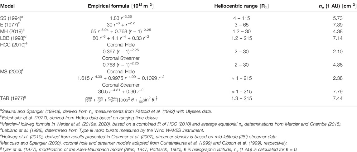
TABLE 1. Empirically-determined coronal plasma density models used in FR studies, their applicable range, and value at 1 AU. Heliocentric distance, r, is given in units of R_⊙.

If there is no independent data for n_e available, then the power-law model is usually selected according to three qualitative guidelines:

1. Heliocentric distances under consideration.

2. Morphology of the coronal structure(s) pierced by the LOS.

3. Phase of the solar cycle (e.g. solar minimum or maximum).

The range of heliocentric distances sampled by FR observations is the most relevant to selecting a power-law model with the appropriate number of terms and power indices. A single-term power law may be used if the range of heliocentric distances is narrow (e.g. 4.6–5.0 R_⊙ in Kooi et al., 2014) or if the heliocentric distance is large (e.g. for LOS beyond 15 R_⊙ in Kooi et al., 2021). Multiple-term power laws are used when the heliocentric range under consideration is large, potentially featuring a term with a large power index (α_i ≥ 6) to represent the inner corona (i.e. below 1.5 R_⊙), a term with a modest power index (2 ≤ α_i ≤ 6) to represent the middle corona out to $\approx 10{\mathrm{R}}_{\odot }$, and/or a term to match the r⁻² fall-off for solar wind out to 1 AU.

The type and variety of coronal structures occulting the LOS is important to selecting a model with the appropriate symmetry and magnitude. If the LOS primarily samples coronal holes, then a spherically-symmetric low-magnitude power law may be sufficient. If the LOS primarily samples the heliospheric current sheet, then a spherically-symmetric large-magnitude power law model may be required. For LOS that pierce a variety of regions (coronal holes, non-equatorial streamers, etc.), asymmetric power-laws are required. The coronal morphology is more important than the phase of solar cycle in selecting an appropriate n_e model for the simple reason that these models can always be re-scaled to conditions of the current solar cycle. Also, modern FR studies typically use independent n_e data to either determine the best empirical model or calculate the best power-law fit to the independent data (see Section 3). For further discussion of empirical models for coronal plasma density, see Bird and Edenhofer (1990).

Table 2 provides references for four analytic-empirical magnetic field strength models that have been used in previous FR observations. Similar to n_e, the magnetic field structure is usually assumed to follow a power-law model, with the number of terms and power indices typically determined by the range in heliocentric distances being investigated. While n_e may or may not be spherically symmetric, the magnetic field is generally assumed to break the symmetry of the corona. In simpler models, this is generally done by assuming a split-monopole form for the vector magnetic field (i.e. a neutral line separates the corona into regions of positive and negative radial magnetic flux), then using the power-law model to determine the magnetic field strength:

$\mathbf{B}\left(r\right)=\sum _i{B}_i{\left(\frac{r}{{\mathrm{R}}_{\odot }}\right)}^{-{\delta }_i}\widehat{{\mathbf{e}}_{\mathrm{r}}}(3)$

At heliocentric distances ≳ 5 R_⊙, a common form used in FR studies (see, e.g. Pätzold et al., 1987; Mancuso and Spangler, 2000; Kooi et al., 2014; Kooi and Kaplan, 2020) is a two-term power law consisting of a dipole term (∝ r⁻³) and an interplanetary magnetic field term (∝ r⁻²):

$\mathbf{B}\left(r\right)=\left[B_1{\left(\frac{r}{{\mathrm{R}}_{\odot }}\right)}^{-2}+B_2{\left(\frac{r}{{\mathrm{R}}_{\odot }}\right)}^{-3}\right]\widehat{{\mathbf{e}}_{\mathrm{r}}}(4)$

The sign of the magnetic field depends on the polarity of the split-monopole. The left image in Figure 1 illustrates such a model, divided into symmetric magnetic sectors. The symmetry lines (dashed and dotted in this figure) are determined by the location at which the LOS crosses the neutral line. If the LOS is parameterized in terms of the coordinate β, with the radio source located at β ≈ − π/2 and the receiver at β ≈ + π/2, this location is given by β_c. At β = 0, the LOS passes closest to the Sun, a distance defined as the impact parameter, R₀. In this example, taken from Kooi et al. (2014), the magnetic flux sector A is positive and the magnetic flux in sectors B, C, and D is negative. Because the geometry of this magnetic field is radial, the contribution to FR in sectors A, C, and D is negative and the contribution to FR in sector B is positive. If n_e is assumed to be spherically symmetric, then the net FR in this configuration is negative.

TABLE 2

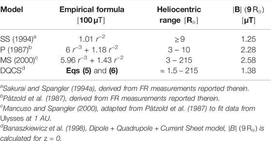
TABLE 2. Magnetic field strength models used in FR studies, their applicable range, and value at 9 R_⊙ (the approximate heliocentric distance Parker Solar Probe will reach during its closest approach in 2024). Heliocentric distance, r, is given in units of R_⊙.

FIGURE 1

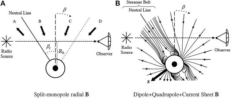
FIGURE 1. Illustrations of coronal magnetic field geometries. In (A), the solid arrows give the orientation of magnetic flux on either side of the neutral line. R₀ is the impact parameter (i.e. where the LOS passes closest to the Sun) and β_c is the location at which the LOS crosses the neutral line (with + β in the direction of the observer). The sectors A, B, C, and D represent regions of symmetry defined by the position of β_c. For the Dipole + Quadrupole + Current Sheet (DQCS) model in (B), there is still a neutral line defined by the current sheet with positive or negative flux on either side; however, the corona is no longer separated into symmetric sectors. The solid arrow gives the z-axis orientation as defined in Banaszkiewicz et al. (1998). Left image appears as Figure 1 in Kooi et al. (2014), ©AAS, reproduced with permission. Right image appears as Figure 4 in Kooi and Kaplan (2020), ©Springer, reproduced with permission.

Below $\approx 5{\mathrm{R}}_{\odot }$, higher order terms are usually necessary (e.g. a quadrupole term). More complex models may also replace the split-monopole and neutral line structure with a physical current sheet that separates the regions of positive and negative (non-radial) magnetic flux, such as the Dipole + Quadrupole + Current Sheet model (DQCS, see Banaszkiewicz et al., 1998). This is illustrated in the right image of Figure 1. This model consists of a dipole term (∝ r⁻³), a weak quadrupole term (∝ r⁻⁵), and replaces the “IMF” term in Eq. (4) with a current sheet term (again, ∝ r⁻²). In cylindrical polar coordinates (ρ and z in solar radii), the DQCS magnetic field model is given by

$\frac{B_{\rho }}{M}=\frac{3\rho z}{r^5}+\frac{15Q}{8}\frac{\rho z}{r^7}\frac{\left(4z^2-3{\rho }^2\right)}{r^2}+\frac{K}{a}\frac{\rho }{{\left[{\left(|z|+a\right)}^2+{\rho }^2\right]}^{3/2}}(5)$

and

$\frac{B_z}{M}=\frac{2z^2-{\rho }^2}{r^5}+\frac{3Q}{8}\frac{\left(8z^4+3{\rho }^4-24{\rho }^2{z}^2\right)}{r^9}+\frac{K}{a}\frac{|z|+a}{{\left[{\left(|z|+a\right)}^2+{\rho }^2\right]}^{3/2}}(6)$

where r² = ρ² + z² is the heliocentric radial coordinate. Eqs (5) and (6) appear as Eqs (1), (2) of Banaszkiewicz et al. (1998). The first, second, and third terms in Eqs (5), (6) are the dipole, quadrupole, and current sheet terms, respectively. The model parameters M = 178.9 μT, Q = 1.5, K = 1.0, and a = 1.538 were selected by Banaszkiewicz et al. (1998) so that the last closed field line intersected the Sun at 60° latitude and the magnitude of the radial magnetic field would be B_r ≈ 3.1 nT at 1 AU. Similar limits at 1 AU are used to scale the split-monopole power-law magnetic fields (e.g. Eq. (4)).

For radially-asymmetric n_e models (e.g. MS (2000) in Table 1), the densest regions (associated with the heliospheric current sheet) are mapped to the neutral line. For some models, such as TAB (1977), the density dependence on heliographic latitude is explicit; however, for models like MS (2000) that divide the corona into dense and tenuous sectors, further assumptions must be made regarding where the dense (i.e. streamer) region ends and the tenuous (i.e. hole or quiet Sun) regions begin. This was typically done either by assuming a streamer belt thickness (e.g $\approx 25$° in Bird et al., 1996; Mancuso and Spangler, 2000; Kooi et al., 2014) or determining a best fit, provided enough FR data is obtained. More recently, Gopalswamy et al. (2021b) demonstrated that the thickness can be determined using time profiles of the polarized brightness in LASCO-C2 synoptic maps.

The complexity of the n_e and B notwithstanding, the two most important parameters necessary for modeling the resulting FR are the impact parameter, R₀ (i.e. where the LOS passes closest to the Sun) and the location at which the LOS crosses the neutral line, β_c. The importance of R₀ and β_c is illuminated by calculating the FR that results assuming a simple single-term, spherically symmetric power law for n_e and a single-term split-monopole power-law for B (i = 1 in Eqs (2) and (3); the corresponding magnitude for the Faraday rotation measure, |RM|, is given by Eq. (4) in Ingleby et al. (2007):

$|\mathrm{R}\mathrm{M}|=\left[\frac{2C_{\mathrm{F}\mathrm{R}}{\mathrm{R}}_{\odot }{N}_1{B}_1}{\left({\alpha }_1+{\delta }_1-1\right){\mathrm{R}}_0^{{\alpha }_1+{\delta }_1-1}}\right]{\cos }^{{\alpha }_1+{\delta }_1-1}\left({\beta }_c\right)(7)$

It is clear that the magnitude depends inversely on R₀; however, |RM| also depends strongly on β_c. For large |β_c|, the RM is effectively zero; consequently, even if the LOS passes close to the Sun, there is still a chance of measuring a zero average contribution from the corona (the corona is constantly fluctuating with, e.g. magnetohydrodynamic (MHD) waves about the average background structure). This also demonstrates that the FR is maximum for |β_c| ≈ 0. In general, |β_c| ≈ 0 occurs when the heliographic latitude of the LOS is similar to the latitudinal position of the heliospheric current sheet (i.e. neutral line) or during times of solar maximum conditions when the heliospheric current sheet is strongly warped.

R₀ is calculated using spherical trigonometry, given the sky coordinates of the Sun and the background radio source. A reliable method to determine β_c is to project the LOS onto a potential-field source-surface (PFSS) synoptic chart for the Carrington rotation corresponding to the FR observations. Jensen (2007) found that the magnetic field values derived from PFSS solutions only vary from Faraday rotation results by a factor of 0.5–2. Synoptic charts can be obtained, for instance, from the Wilcox Solar Observatory (WSO). WSO provides three versions of these charts¹ for a given Carrington rotation:

1. “classic” version assuming the photospheric field has a meridional component and requiring an ad hoc polar field correction, with the source surface located at 2.5 R_⊙;

2. “radial” version assuming a radial field and no polar field correction, with the source surface located at 2.5 R_⊙;

3. “radial” version with the source surface located at 3.25 R_⊙.

Mancuso and Garzelli (2013) concluded that the radial version with the source surface located at 2.5 R_⊙ provides the best FR model fit during solar minimum conditions. PFSS model synoptic maps are also available² from the National Solar Observatory’s Global Oscillations Network Group (GONG, Hill, 2018) magnetograms. Details concerning this method are discussed in Mancuso and Spangler (2000) and Ingleby et al. (2007).

Figure 2 demonstrates the calculation of β_c for observations reported in Kooi et al. (2014). The left panel in Figure 2 shows the sky position of the radio source, 3C 228, in relation to the Sun. The right panel in Figure 2 demonstrates the output of an algorithm to calculate β_c. The original observations, reported in Kooi et al. (2014), were made during solar maximum conditions in 2011; consequently, the neutral line covers a broad range in heliographic latitude. By contrast, the neutral line typically covers a much smaller range during solar minimum conditions. Here, β_c ≈ − 33° can be read directly from the chart where the neutral line (dotted line) crosses the LOS (solid black line). β_c = 0° gives the heliographic latitude and Carrington longitude of the LOS position in the sky plane. Because this process involves mapping the LOS onto a sphere, LOS corresponding to large latitudes in the sky plane (i.e. the LOS in Figure 2) show significant curvature; whereas LOS at near-equatorial latitudes appear relatively flat (see, e.g., the Field 1 LOS in Figure 5 of Kooi et al., 2021).

FIGURE 2

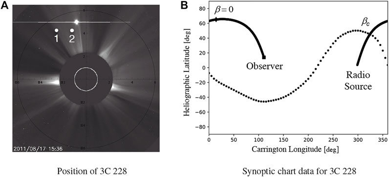
FIGURE 2. Position of radio galaxy 3C 228 during coronal FR observations on 2011 August 17 reported in Kooi et al. (2014) (A) and the LOS to 3C 228 mapped onto synoptic chart data to calculate β_c (B). Positions of 3C 228 near the beginning (“1”) and end (“2”) of the 8-h observations are plotted on a LASCO-C2 coronagraph image, along with a white circle to represent the Sun’s position. The bright source north of the LOS is Venus. In the right panel, the solid line is the projected LOS to 3C 228 in heliographic latitude and Carrington longitude. Dotted line gives the location of the magnetic neutral line as determined by the WSO radial model with source surface at 3.25 R_⊙. The solid square is the heliographic projection of the observer (Earth, β =180°), the solid diamond gives the midpoint of the LOS (β =0°), and β_c is measured where the LOS and neutral line intersect (−33°). Left image appears as Figure 3 in Kooi et al. (2014) and is publicly available at https://sohowww.nascom.nasa.gov/. Right image appears as Figure 11 in Kooi and Kaplan (2020), ©Springer, reproduced with permission.

Qualitatively, if the LOS depicted in Figure 2 was, instead, located near the heliographic equator, β_c ≈ 10° and the observed FR would be much larger than the values of −20 to +30 rad m⁻² reported in Kooi et al. (2014). Alternately, if these observations were made during solar minimum conditions when the neutral line is typically restricted to heliographic latitudes $<20$°, then β_c > 70° and, therefore, the magnitude of the FR would be dramatically reduced (e.g. Eq. (7)).

Two issues can arise using synoptic charts similar to the one in Figure 2 to calculate β_c:

1. Synoptic-chart data from two separate Carrington rotations will be available for a given set of observations.

2. The position of the neutral line (i.e. heliospheric current sheet) evolves rapidly during a single Carrington rotation.

In both cases, the evolution of the neutral line can dramatically change the value of β_c. The first issue was encountered during the aforementioned 2011 observations; Kooi et al. (2014) used synoptic data from both Carrington rotations 2,113 and 2,114 to provide a range for β_c (≈−33° to ≈ −42°), and noted that the true value likely lies somewhere within this range. The second issue was encountered during observations in 2015, reported in Kooi et al. (2021). Due to a series of dramatic CME events, the heliospheric current sheet evolved quickly over 24 h off the eastern limb of the Sun. To model this effect, Kooi et al. (2021) dynamically evolved the corresponding neutral line in synoptic chart data to match the observed motion in coronagraph images from LASCO-C2 and LASCO-C3. The maximum deviation of the neutral line position from synoptic data as well as the rate at which to evolve the neutral line were determined from coronagraph images and, therefore, subject to projection effects; in particular, there was an ambiguity in the Carrington Longitude coordinates of the evolving heliospheric current sheet. This ambiguity was resolved using the Faraday rotation observations themselves (see Figure 5 in Kooi et al., 2021, and discussion therein). Due to this position ambiguity, this method would be difficult to implement in general cases without Faraday rotation measurements or, e.g. stereoscopic white-light imaging.

2.2 Flux Rope Models for CME Plasma Density and Magnetic Field

In cases where coronal FR studies were fortunate enough to detect FR through CMEs, the primary morphology used to describe the CME structure is the flux rope. Helical flux rope magnetic field configurations have been measured in situ over generations of spacecraft missions (e.g. see discussions in Burlaga et al., 1981; Burlaga, 1988; Lepping et al., 1990; Marubashi et al., 2015; Nieves-Chinchilla et al., 2019); such configurations also explain the white-light morphology seen in space-borne coronagraphs (Chen, 1996; Gibson and Low, 1998; Gibson and Low, 2000; Gibson et al., 2006). Relative to the classical three-part structure of CMEs, most models of CMEs tend to associate the dim inner cavity with the flux rope (e.g. Low, 2001).

CME FR has been modeled using both force-free $\left(\nabla \times \mathbf{B}=\alpha \mathbf{B}\right)$ and non-force-free $\left(\mathbf{J}\times \mathbf{B}=\nabla p\right)$ magnetic flux ropes (see for instance, Hidalgo et al., 2000; Nieves-Chinchilla et al., 2016, Nieves-Chinchilla et al., 2018; Hu, 2017). As discussed in Liu et al. (2007), both types can:

1. reproduce the signs and magnitudes of CME FR;

2. produce the same variety of CME FR profiles;

3. generate similar FR profiles for a given orientation with respect to the LOS;

consequently, most CME FR observations have been interpreted using the simpler force-free flux rope structure. Jensen and Russell (2008) demonstrated that the basic profiles of previous CMR FR observations (Levy et al., 1969; Cannon et al., 1973; Bird et al., 1985) could be reproduced using a force-free flux rope. In exploring these models, both Liu et al. (2007) and Jensen and Russell (2008) came to an important conclusion: multiple LOS are necessary for resolving ambiguities in the orientation and helicity of the CME B, which we discuss further in Section 5.

The “standard” force-free flux rope used in observational FR studies is composed of a cylindrically symmetric axial and azimuthal field (e.g., see Gurnett and Bhattacharjee, 2006):

$\mathbf{B}=B_{cme}\left[J_0\left(\alpha \rho \right){\widehat{\mathbf{e}}}_{\mathbf{z}}+H{J}_1\left(\alpha \rho \right){\widehat{\mathbf{e}}}_{\mathit{\varphi }}\right](8)$

where B_cme and H are the magnitude of the axial magnetic field and helicity (H = ±1, where + is right-handed and − is left-handed). J₀ and J₁ are the zeroth- and first-order Bessel functions of the first kind, respectively. Axis-centered cylindrical coordinates are given as $\left({\widehat{\mathbf{e}}}_{\mathit{\rho }},{\widehat{\mathbf{e}}}_{\mathit{\varphi }},{\widehat{\mathbf{e}}}_{\mathbf{z}}\right)$. For a flux rope with radius R_cme, we define αR_cme ≡ 2.405, the first zero of J₀, to ensure that the axial field is zero at the surface of the flux rope. While the LOS is typically assumed to extend from source to observer for coronal FR modeling, the effective LOS length used for CME FR analysis is simply the LOS length contained within the CME flux rope structure itself. Jensen et al. (2010) explored the wide variety of possible FR profiles for flux ropes determined by their geometric orientation with respect to the LOS. Figure 3 illustrates some of these profiles, from “U” shapes to “W” shapes to “N” shapes. For more details, the coordinate system definition, and more profiles, see Jensen et al. (2010).

FIGURE 3

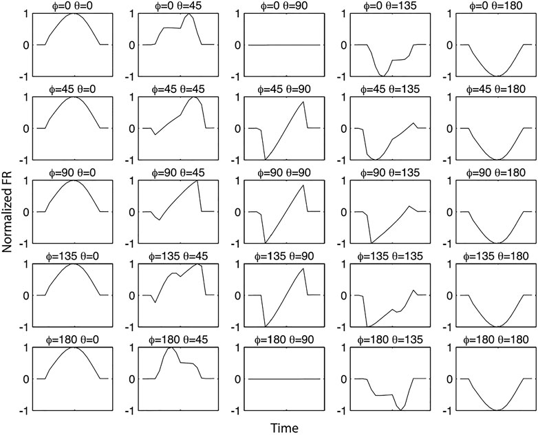
FIGURE 3. Range of possible normalized FR profiles for a magnetic flux rope configuration with right-handed helicity. ϕ and θ are spherical angles that give the orientation of the axial magnetic field vector. ϕ is the clock angle, which increases from 0° along the y-axis to 90° along the z-axis. θ is the cone angle, which is the offset angle from the y-z plane. This appears as Figure 6 in Jensen et al. (2010), ©The Authors under the Creative Commons license (https://creativecommons.org/licenses/by/2.0/), reproduced with permission.

Previous modeling efforts have assumed infinite flux rope cylinders (Kooi et al., 2017) as well as finite-length cylinders (Liu et al., 2007; Jensen and Russell, 2008; Jensen et al., 2010; Kooi et al., 2021); however, all modeling efforts thus far have treated CMEs as cylinders on the scale of the LOS that penetrates the CME, no attempts have been made to account for the CME’s curvature on global scales. This is a consequence of the sparse sampling of LOS probing a CME. Observations of CME FR are rare to begin with and only Kooi et al. (2021) have reported observations of CME FR utilizing multiple LOS. In order to measure the curvature and other fine scale attributes of CMEs, coronal FR studies need to develop the capability to measure FR simultaneously along hundreds or even thousands of lines of sight.

Liu et al. (2007) and Jensen et al. (2010) both simulated sky maps of FR through CMEs to showcase the power of multiple LOS. The left panels in Figure 4 show FR sky maps corresponding to the four configurations of the axial magnetic field and helicity that are possible for a given geometric orientation of the flux rope position in space. This figure is equivalent to assuming an FR measurement can be made for each pixel in the image (i.e. 100s or 1000s of FR measurements). If only a few LOS are available over a relatively small patch of sky, this will narrow down the possible orientations to two; e.g. if the LOS are located near θ_z = 1.5° and θ_y = 0°, then it is impossible to distinguish between the left-handed helicity with B_z pointing in the positive θ_y direction and the right-handed helicity with B_z pointing in the negative θ_y direction. Jensen et al. (2010) simulated the FR sky maps for CMEs as well as the potential interference of a sheath as they would be seen by the Murchison Widefield Array (MWA) using many LOS, at a 50-min cadence. One such example for the “Halloween Event” on 2003 October 28, is shown in the right panel of Figure 4.

FIGURE 4

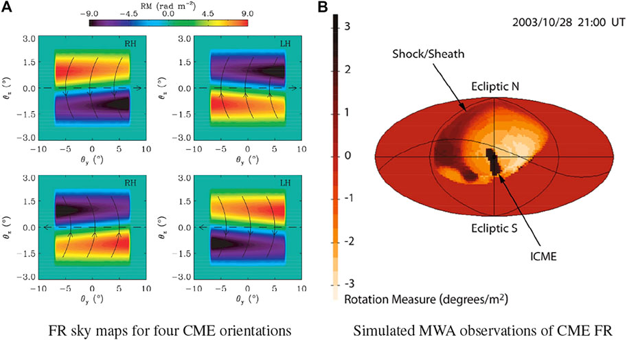
FIGURE 4. Simulated sky maps of FR for different magnetic flux rope configurations. In (A), for a given geometric orientation with respect to the LOS, there are four possible configurations for the axial magnetic field (dashed arrow) and helicity (solid curved lines), which generate a range of Faraday rotation measure (RM) values. Panel (B) shows the expected FR for a CME on 2003 October 28 as seen by the MWA. Both simulations demonstrate the powerful potential for FR observations to probe the magnetic structure of CMEs given many LOS are available. Left image appears as Figure 6 in Liu et al. (2007), ©AAS, reproduced with permission. Right image appears as Figure 11 in Jensen et al. (2010), ©The Authors under the Creative Commons license (https://creativecommons.org/licenses/by/2.0/), reproduced with permission.

Within the flux rope structure, n_e is usually assumed to be constant and is either fixed using assumptions about plasma β (e.g. in modeling from Liu et al., 2007) or solved using independent white-light data (Section 3.2 and Section 5.2). Because they observed multiple LOS sampling different regions of the CME, Kooi et al. (2021) compared three different models for n_e: constant density, thin shell, and thick shell models. The constant density and thin shell models performed equally well and provided better fits to the data than the thick shell model.

3 Using Independent Plasma Density Data to Complement FR Studies

One of the greatest steps forward for modern coronal FR studies has been to implement independent data for n_e into FR observations. We highlight here the most recent methods used to extract information about the coronal n_e to complement FR studies. Application of these methods depends primarily on the background radio source: dispersion measurements for background pulsars; Thomson scattering brightness measurements for background radio galaxies; and radio ranging and apparent-Doppler tracking for background spacecraft. Scintillation observations can also be used (Bisi et al., 2021); however, we are focusing on direct LOS measurement in this section.

3.1 Dispersion Measurements Using Pulsars

A rather underutilized method in coronal FR studies to determine n_e along the LOS involves calculating the dispersion measure, DM:

$\mathrm{D}\mathrm{M}\equiv {\int }_{\text{LOS}}{n}_{\mathrm{e}}\left(s\right)\mathrm{d}\mathrm{s}(9)$

where the LOS is the full distance from a background pulsar to the observer. Pulsars result from a highly magnetized, rapidly rotating neutron star. In essence, the radio emission is beamed out along the axis of the magnetic field and every time the star rotates, this beam passes Earth’s LOS (provided the magnetic field is not aligned with the rotational axis). Pulsars were first suggested as a background source for coronal investigations by Hollweg (1968) and Counselman et al. (1968). An important advantage to using pulsars as the background emission source is that the interval between pulses (the “off” phase of the pulsar) can be used to calibrate the background emission, including solar interference in the side lobes of the antenna (see, e.g. Bird et al., 1980).

The key feature of pulsars (and millisecond pulsars, MSPs, in particular) is that the RM and DM can be simultaneously measured. Because the DM is simply proportional to the LOS integral over plasma density, it provides the independent data necessary to disentangle the effects of n_e and B_∥ in FR observations. At distances of 5–20 R_⊙, the coronal DM can be a factor of 10³–10⁴ times smaller than the interstellar DM (e.g. You et al., 2012; Howard et al., 2016); consequently, MSPs make ideal candidates because they can be timed with a precision on the order of 100 ns (Manchester et al., 2013). For example, Madison et al. (2019) used observations of solar wind perturbations to DM toward a large number of MSPs to characterize the large-scale density structure of the solar wind (see also Tiburzi et al., 2021).

However, results for coronal FR studies using pulsars and MSPs have only been reported in three papers over the last couple decades: Ord et al. (2007), You et al. (2012), and Howard et al. (2016). In particular, You et al. (2012) exploited observations of PSR J1022 + 1001 made as part of the Parkes Pulsar Timing Array (PPTA) project to measure RM and DM at source elongations ranging from 6.2–19 R_⊙. These were used to estimate the coronal magnetic field within the context of existing coronal and solar wind models. Importantly, You et al. (2012) showed that the availability of simultaneous measurements of the DM provided strong constraints on the coronal and solar wind density models and that errors introduced by assumptions made in the absence of DM measurements were significantly greater $(\approx 50\%)$ and dominated the error budget.

3.2 Simultaneous Thomson Scattering Brightness Measurements From Space-Borne Coronagraphs

Observations of radio galaxies at offsets sufficiently close to the Sun can take advantage of space-borne coronagraphs that observe radiation from the photosphere that has been Thomson-scattered by electrons in the coronal plasma. Thomson scattering brightness, TSB, is directly related to n_e by a LOS integral weighted by a geometric function, $\mathcal{G}(\mathbf{r})$, whose form is determined by assumptions about solar limb darkening and heliocentric distance:

$\mathrm{T}\mathrm{S}\mathrm{B}={\int }_{LOS}{n}_{\mathrm{e}}\left(\mathbf{r}\right)\mathcal{G}\left(\mathbf{r}\right)dr(10)$

where r is vector heliocentric distance. The full form of $\mathcal{G}(r)$ (given as Eq. (17) in van de Hulst, 1950) is

$\mathcal{G}\left(r\right)=\left(\frac{3}{4}{\sigma }_{\mathrm{T}}{\mathrm{R}}_{\odot }{\mathrm{B}}_{\odot }\right)\left[\left(2-\frac{R_0^2}{r^2}\right)\mathcal{A}\left(r\right)+\frac{R_0^2}{r^2}\mathcal{B}\left(r\right)\right]\frac{r}{\sqrt{r^2-R_0^2}}(11)$

where σ_T, R_⊙, and B_⊙ are the Thomson scattering cross-section, solar radius, and mean surface brightness of the Sun. r is the heliocentric distance to a given point along the LOS at which scattering occurs and R₀ is the impact parameter for the LOS as before (both given here in units of R_⊙). $\mathcal{A}(r)$ and $\mathcal{B}(r)$ are geometric factors and discussed in detail in van de Hulst (1950).

$\mathcal{A}(r)$ and $\mathcal{B}(r)$ rapidly approach the limits $\mathcal{A}(r)\to 1/2r^{-2}$ and $\mathcal{B}(r)\to 0$ as r → 5 R_⊙. Redefining Eqs (10), (11) in terms of the β angle defined in Section 2.1 gives

$\mathrm{T}\mathrm{S}\mathrm{B}=\left(\frac{3{\sigma }_{\mathrm{T}}{\mathrm{R}}_{\odot }{\mathrm{B}}_{\odot }}{16R_0}\right){\int }_{-\pi /2}^{\pi /2}\left[1+{\sin }^2\left(\beta \right)\right]n_e\left(R_0,\beta \right)d\beta (12)$

Eq. (12) assumes the LOS length is the full distance from a given background radio galaxy to the observer at Earth; any contributions to the optical brightness of coronagraph images from sources other than the electron corona are either removed using model-subtraction methods (e.g. for local stars that may intersect the LOS) or negligible (e.g. from the background radio galaxy itself). If n_e has a power-law form given by Eq. (2), the corresponding TSB is

$\mathrm{T}\mathrm{S}\mathrm{B}=\sum _i\left(\frac{3{\sigma }_{\mathrm{T}}{\mathrm{R}}_{\odot }{\mathrm{B}}_{\odot }{N}_i}{8}\right)R_0^{-{\alpha }_i-1}\left(\frac{\sqrt{\pi }}{1+{\alpha }_i}\right)\frac{\mathrm{\Gamma }\left(\frac{5}{2}+\frac{{\alpha }_i}{2}\right)}{\mathrm{\Gamma }\left(2+\frac{{\alpha }_i}{2}\right)}(13)$

which is equivalent to Eq. (7) in Kooi et al. (2017). Eq. (13) can then be fitted to TSB coronagraph data for a given LOS to determine the coefficients N_i and power indices α_i.

van de Hulst (1950) developed the original method of deriving coronal n_e by inverting polarized brightness measurements. Hayes et al. (2001) then extended this method to total brightness observations. This has provided the ability to determine n_e contributions to FR using white-light coronagraphs such as the Large Angle and Spectrometric Coronagraph (LASCO; Brueckner et al., 1995) on board the Solar and Heliospheric Observatory (SOHO; Domingo et al., 1995) and the Sun-Earth Connection Coronal and Heliospheric Investigation (SECCHI; Howard et al., 2008) instrument suites on board the twin Solar TErrestrial RElations Observatory (STEREO; Kaiser et al., 2008) spacecraft. However, because the K corona (coronal electron plasma) and F corona (scattering off interplanetary dust) both contribute to the total brightness, the accuracy of deriving n_e from total brightness observations depends strongly on the accuracy of the removal of the brightness contributions from the F corona. For discussion of how this is done for coronal FR studies, see Kooi et al. (2017) and references therein.

This method has worked well in previous observations of coronal FR (e.g. Howard et al., 2016; Kooi et al., 2017, Kooi et al., 2021), but relies primarily on the SOHO LASCO coronagraphs because SOHO orbits the Sun-Earth L1 point, its observational perspective is essentially the same as a radio receiver’s on Earth; therefore, it is straightforward to map radio LOS through the LASCO coronagraph field-of-view. SOHO currently has two operational coronagraphs, C2 and C3, with a field-of-view of 1.5–6.0 R_⊙ and 3.7–30 R_⊙, respectively (Brueckner et al., 1995). As a result, FR observations of the middle and outer corona tend to use LASCO-C2 and C3, respectively.

However, care should be taken if the LOS is near the inner or outer boundary of the field-of-view. Near the inner boundary, where the K corona is brightest, most F corona subtraction methods can lead to subtraction of a portion of the K corona as well. This can be especially true if the K corona is quasi-static as is often the case during solar minimum conditions. Near the outer boundary, the TSB signal becomes noise-dominated. Most observations in the outer corona are made at heliocentric distances $<20{\mathrm{R}}_{\odot }$ and are not noise-dominated unless the LOS is located in a particularly white-light dim coronal hole. For observations near the outer boundary of the middle corona $(\approx 6{\mathrm{R}}_{\odot })$, it is usually best to calculate a radial power-law model for n_e across the C2 field-of-view similar to Hayes et al. (2001), instead of fitting the TSB data along the LOS.

3.3 Radio Ranging and Apparent-Doppler Tracking Methods

For spacecraft, radio ranging and apparent-Doppler tracking methods can be employed. These two methods provide a measure of the Total Electron Content, TEC, of the coronal plasma:

$\mathrm{T}\mathrm{E}\mathrm{C}\equiv {\int }_{\mathrm{L}\mathrm{O}\mathrm{S}}{n}_{\mathrm{e}}\left(s\right)\mathrm{d}\mathrm{s}(14)$

While similar in form to the DM in Eq. (9), the TEC specifically refers to the column density of electrons in the corona, whereas the DM includes not only the corona, but also the interstellar medium.

Radio ranging (also known as Differenced Ranging Versus Integrated Doppler, DRVID), measures the group delay time required to send a wave packet from the spacecraft to the observer. The group delay time, Δt, for a signal with angular frequency ω is directly related to the TEC by

$\mathrm{\Delta }t=\frac{S}{\mathrm{c}}+\frac{q_{\mathrm{e}}^2}{2{\omega }^2\mathrm{c}{ϵ}_0{\mathrm{m}}_e}\mathrm{T}\mathrm{E}\mathrm{C}(15)$

where c, q_e, ϵ₀, and m_e are the physical constants representing the speed of light, electron charge, permittivity of free space, and electron mass, respectively. S ≡∫_LOSds is the effective length of the LOS; consequently, the time delay added to the signal due the dispersive coronal plasma is represented by the second term. This appears as Eq. (7) in Jensen et al. (2016). Beyond providing a direct measurement of the TEC, radio ranging can also be used to study fractional electron density fluctuations (see, e.g. Woo et al., 1995).

The apparent-Doppler tracking method relies on measuring the frequency, independent of Doppler motion that results from the spacecraft traveling dS/dt, of a transmitted signal through a gradient in n_e. For a given frequency, f, the frequency shift, Δf, is effectively given by the time derivative of Eq. (15):

$\frac{\mathrm{\Delta }f}{f}=-\frac{1}{\mathrm{c}}\frac{\mathrm{d}S}{\mathrm{d}\mathrm{t}}+\frac{q_{\mathrm{e}}^2}{2{\omega }^2\mathrm{c}{ϵ}_0{\mathrm{m}}_e}\frac{\mathrm{d}}{\mathrm{d}\mathrm{t}}\mathrm{T}\mathrm{E}\mathrm{C}(16)$

This appears as Eq. (11) in Jensen et al. (2016). This technique works best when there are multiple frequencies available. For two or more frequencies, the spacecraft Doppler motion can be removed via subtraction because it contributes equally to all frequencies. The remaining frequency-dependent fluctuations are therefore a result of the plasma. Simultaneously measuring the absolute TEC with ranging also provides a more accurate measure of the TEC within the exact Fresnel space as the signal when tracking the changes in TEC with these frequency fluctuations. If only one frequency is available, though, JPL/NAIF SPICE ephemeris³ calculations can be used to eliminate the expected spacecraft motion, with much less accuracy.

Jensen et al. (2016) explored both methods for measuring TEC as a function of time using the Cassini spacecraft as the background radio source. In this case, the uplink frequency was a monochromatic sinusoidal signal at 7.2 GHz and Cassini broadcast at two, phase-locked sinusoidal signals of 8.4 and 32 GHz. Having successfully demonstrated the efficacy of these methods for measuring TEC, Jensen et al. (2018) later applied these techniques to FR observations of a CME observed on 2013 May 10 using the MErcury Surface, Space ENvironment, GEochemistry, and Ranging (MESSENGER) spacecraft (see Section 5.1). Ranging and apparent-Doppler methods will also be used to measure the TEC coinciding with FR measurements made by the Faraday Effect Tracker of Coronal and Heliospheric structures (FETCH) instrument as part of the Multiview Observatory for Solar Terrestrial science (MOST: Gopalswamy et al., 2021a) mission concept discussed in Section 6.3.

4 Modern Contributions to Understanding the Corona

While numerous FR experiments over the last few decades have continued to return estimates for the large-scale magnetic field, we focus our discussion here on two truly novel methods that have been developed to use FR to probe coronal magnetic field fluctuations and electric currents.

4.1 FRF and Faraday Screen Depolarization Implications for Wave-Turbulence Heating

One of the most active areas of research in modern solar physics is identifying the mechanism(s) responsible for heating the corona to temperatures over a million kelvin. FR observations can provide unique insights into models for coronal heating mechanisms and, in particular, can provide constraints on models of wave-dissipation heating. Wave-dissipation models usually assume that wavelike oscillations within the corona (e.g. Alfvén waves) are damped out, typically by invoking turbulence, and the wave power is translated into energy that can heat the corona and drive solar wind acceleration. In wave-dissipation models, the wave flux density required is around 200–500 W m⁻² (Hollweg et al., 2010).

Measurement of FR fluctuations (FRF) is one of the few methods available for detecting and providing estimates for the wave power within the corona. Perturbations in n_e or magnetic field structure can, in principle, produce wavelike structures detectable in the variance of FR measurements. Simultaneous observations of FRF and electron content variations (Hollweg et al., 1982), as well as comparisons of experimental results with theoretical models (Chashei and Shishov, 1983; Chashei and Shishov, 1984; Chashei and Shishov, 1986) indicate that magnetic field fluctuations dominate the variance. Consequently, the term that dominates the variance in RM is given by:

$⟨\delta {\mathrm{R}\mathrm{M}}^2⟩\approx C_{\text{FR}}{\int }_{LOS}{n}_{\mathrm{e}}^2⟨\delta B_{\parallel }^2⟩L_{B_{\parallel }}\mathrm{d}\mathrm{s}(17)$

where $⟨\delta B_{\parallel }^2⟩$ is the variance in B_∥ amplitude and $L_{B_{\parallel }}$ is the auto-correlation scale length (see Hollweg et al., 1982, for details).

Eq. (17) is the basis for estimating the amplitude and form of the RMS magnetic field fluctuations, ${⟨\delta B_{\parallel }^2⟩}^{1/2}$, using direct measurements of FRF. While Eq. (17) may appear simple in form, the exact forms for n_e, $⟨\delta B_{\parallel }^2⟩$, and $L_{B_{\parallel }}$ are unknown. As mentioned in Section 2, models for these values are assumed if independent information is not available. Typically, the corona is assumed to be spherically symmetric and the quantities are assumed to vary as power laws in heliocentric distance.

The auto-correlation scale length for the magnetic field, $L_{B_{\parallel }}$, is one of the most difficult quantities to estimate in Eq. (17). Hollweg et al. (1982) assumed that the Alfvén waves were generated by perturbing magnetic flux tubes at the photosphere. As such, they approximate $L_{B_{\parallel }}$ as the mean spacing between flux tubes (e.g. see Spruit, 1981), which is a function of the background magnetic field. Mancuso and Spangler (1999) used the same assumption as Hollweg et al. (1982), as well as estimating $L_{B_{\parallel }}$ based on their measured auto-correlation time and a range of values for the solar wind. They suggested that $L_{B_{\parallel }}$ might be underestimated by a factor of 5–10, which implies that they (along with Hollweg et al., 1982) may have overestimated ${⟨\delta B_{\parallel }^2⟩}^{1/2}$ by the same factor. Wexler et al. (2020) used a correlation length of 10,000 km in middle-corona studies of radio frequency fluctuations, and 5,000 km in an earlier study of FRF below 2 R_⊙ (Wexler et al., 2017). The matter needs further study.

Once estimates for the amplitude $\delta B_{\parallel }\equiv {⟨\delta B_{\parallel }^2⟩}^{1/2}$ and the correlation length have been determined, the wave flux density for Alfvén waves can be calculated as

$F_{\mathrm{A}}=\frac{1}{{\mu }_0}\delta B_{\parallel }^2{V}_{\mathrm{A}}(18)$

in W m⁻², where µ₀ is the permeability of free space and V_A is the Alfvén wave speed. After demonstrating that FRF were associated primarily with fluctuations in the magnetic field, Hollweg et al. (1982) concluded that the wave flux density associated with their FRF measurements was large enough to drive coronal heating through turbulent dissipation. Efimov et al. (1993), Andreev et al. (1997), Jensen and Russell (2008), and Hollweg et al. (2010) similarly concluded that the FRF detected using Helios as the background radio source were consistent with coronal magnetic field fluctuations of sufficient amplitudes to power the solar wind. Limited FRF data over the 1.63–1.89 R_⊙ range (Wexler et al., 2017) suggested an Alfvén wave energy flux of only 7 W m⁻², while similar analysis in stronger magnetic field regions at similar coronal heights revealed energy fluxes in the 35–49 W m⁻² range (Wexler, 2020). When comparing such FRF studies, the spectral range under study needs to be considered. Since the FRF power spectrum has a negative power law index, extension far into the sub-mHz range will produce a much larger RMS δB_∥ and thus higher wave energy flux, but at the risk of detecting slowly-evolving large-scale structure rather than MHD oscillations.

FRF measurements using natural radio sources (i.e. radio galaxies), have only provided upper limits for turbulent wave-dissipation models. Sakurai and Spangler (1994a) calculated the wave flux at the coronal base to be $<160$ W m⁻² and Mancuso and Spangler (1999) inferred a wave flux that ranges from 24 to 230 W m⁻². These observations place restrictions on the low frequency Alfvén waves (of order a few mHz) seen in the corona, but these waves may or may not be directly correlated with the high frequency ($\approx 1-100$s of Hz) Alfvén waves thought to be associated with heating the corona. Spangler and Mancuso (2000) developed a possible method for examining these high frequency waves through the observation of Faraday screen depolarization. The basic idea is that the antenna beam used to observe an extended radio source through the corona (or any medium) has a finite footprint on this region roughly proportional to the product of the beam’s half-width and the distance to the region. A high level of high frequency Alfvén waves in the corona could produce many regions of uncorrelated FRF within the beam’s footprint, reducing the net polarization detected at the receiver. Spangler and Mancuso (2000) argued that depending on the exact properties of the high frequency wave dissipation models employed, a detectable depolarization of $\approx 5-20\%$ should result; however, they found no detectable depolarization.

More recent observations also showed no detectable depolarization of extended radio sources (e.g. see Spangler and Spitler, 2005; Spangler and Whiting, 2009). These observations were primarily focused on constraining the amplitude and outer scales of turbulent dissipation processes: turbulence with an amplitude of δB/B ≈ 0.2–0.3 should have an outer scale on the order of the beam footprint (1000 − 2000 km) and turbulence with a larger amplitude of δB/B ≳ 0.5 should have an outer scale much smaller than the beam footprint ($<200$ km). While restrictive, these values agree well with limits suggested by some turbulent wave-dissipation models (e.g. see Hollweg et al., 2010).

4.2 DFR Measurements of Coronal Electric Currents

Electric currents are ubiquitous in the corona, from the large scales of the heliospheric current sheet (HCS, see, e.g., Wilcox and Ness, 1965; Gleeson and Axford, 1976; Koskela et al., 2018) to the smaller scales of current filaments and turbulent current sheets generated by reconnection events (see, e.g., Vaiana et al., 1973; Habbal and Withbroe, 1981; Büchner, 2006; Spangler, 2007). The dissipation of electric currents has also been suggested as a possible mechanism for coronal heating (see, e.g., Heyvaerts and Priest, 1984). Spangler (2007) adapted a method of measuring the magnitudes of coronal currents using differential Faraday rotation (DFR). This method had been previously employed by Brower et al. (2002) and Ding et al. (2003) to measure the internal currents in a laboratory plasma (the Madison symmetric torus, MST, reversed-field pinch, RFP, at the University of Wisconsin, see Prager, 1999) without perturbing the plasma with a physical probe.

DFR is defined as the difference between FR along two or more closely spaced LOS. If the background radio source provides two LOS, e.g. a radio double with Hotspot A and Hotspot B, then the differential Faraday-rotation measure, ΔRM, is defined by

$\mathrm{\Delta }\mathrm{R}\mathrm{M}\equiv {\mathrm{R}\mathrm{M}}_{\mathrm{A}}-{\mathrm{R}\mathrm{M}}_{\mathrm{B}}(19)$

If a “rotation-measure Amperian loop” is set up as in Figure 5, then ΔRM can be well approximated by the sum of all four contributions because the contributions from RM₂ and RM₄ are negligible:

1. the path length of integration for RM₂ and RM₄ is very small because the two LOS are, by definition, closely spaced;

2. the integration paths for RM₂ and RM₄ are considered to be far from the Sun and, consequently, the coronal contribution to n_e and magnetic field will be inconsequential.

FIGURE 5

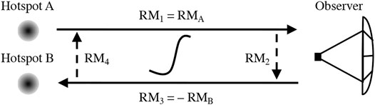
FIGURE 5. Differential Faraday-rotation measurement geometry for a background radio source that provides two LOS (solid arrows): Hotspot A and Hotspot B. The dashed arrows represent the two LOS (with negligible RM) necessary to complete the “rotation-measure Amperian loop.” The curved line enclosed by the loop represents a coronal current detected with this measurement. This appears as Figure 1 in Kooi and Kaplan (2020), ©Springer, reproduced with permission.

Therefore ΔRM can be computed as a closed-loop integration:

$\mathrm{\Delta }\mathrm{R}\mathrm{M}={\mathrm{R}\mathrm{M}}_1+{\mathrm{R}\mathrm{M}}_2+{\mathrm{R}\mathrm{M}}_3+{\mathrm{R}\mathrm{M}}_4=C_{\text{FR}}{\oint }_{\text{LOS}}{n}_{\mathrm{e}}\mathbf{B}\cdot \mathrm{d}\mathbf{s}(20)$

If the region where the measured ΔRM is dominated by a relatively uniform n_e (given by ${\bar{n}}_{\mathrm{e}}$), then Ampere’s law gives the relation between DFR and the current, I_enc, enclosed by the “rotation-measure Amperian loop” in Figure 5 (Spangler, 2007). In SI units:

$\mathrm{\Delta }\mathrm{R}\mathrm{M}\approx C_{\text{FR}}{\bar{n}}_{\mathrm{e}}{\oint }_{\text{LOS}}\mathbf{B}\cdot \mathrm{d}\mathbf{s}=C_{\text{FR}}{\bar{n}}_{\mathrm{e}}{\mu }_0{I}_{\text{enc}}(21)$

where µ₀ is the permeability of free space and C_FR = 2.631 × 10^–13 rad T⁻¹.

DFR results using the radio galaxy 3C 228 as a background radio source were reported by Spangler (2007) and Kooi et al. (2014). 3C 228 is a double radio source with strongly polarized northern and southern hotspots (see Figure 2 in Kooi et al., 2014), permitting DFR measurements along two LOS separated by 46″ on the sky (with a corresponding physical distance of $\approx \mathrm{33,000}\mathrm{k}\mathrm{m}$ in the corona). Spangler (2007) detected ΔRM corresponding to current magnitudes of 0.23–2.5 GA at heliocentric distances of 5.2–6.7 R_⊙. Kooi et al. (2014) measured slightly larger values of 2.6–4.1 GA at heliocentric distances of 4.6–5.0 R_⊙. Spangler (2007) and Kooi et al. (2014) both concluded that the magnitude of the currents detected were insufficent for coronal heating unless the true resistivity in the corona exceeds the Spitzer value by several orders of magnitude.

Spangler (2007) also modeled the expected DFR due to coronal current filaments with a Z-pinch structure (Gurnett and Bhattacharjee, 2006), which is a solution to the mechanical equilibrium requirement that

$\mathbf{J}\times \mathbf{B}-\nabla p=0(22)$

where J and B are the vector current density and magnetic field and p is the plasma pressure. The Z-pinch structure is an unstable equilibrium solution, so it is entirely possible for these filaments to form in turbulent plasmas like the corona and propagate along with the solar wind, then disappearing only to reform further upstream or downstream in the solar wind. In particular, Spangler (2007) found that the error between the true value for the magnitude of the current filament and the value estimated from Eq. (21) was only 37%, supporting the credibility of this remote-sensing method.

More recently, Kooi and Kaplan (2020) investigated the expected DFR associated with the large-scale HCS and found that the HCS DFR depended strongly on the impact parameter, R₀, and the location where the LOS intercepts the HCS, β_c, but was rather insensitive to the small offset between the two LOS. Kooi and Kaplan (2020) also showed that the HCS accounted for up to 10–20% of the observed ΔRM reported by Spangler (2007) and that the small bias in DFR measurements detected on all three days reported in Spangler (2007) and Kooi et al. (2014) was fully consistent with the expected contribution from the HCS. The most important conclusion reported in Kooi and Kaplan (2020), though, was that DFR measurements can provide a more accurate probe of the difference between coronal magnetic field models compared to single LOS measurements of FR alone, especially at heliocentric distances $<5{\mathrm{R}}_{\odot }$. Consequently, future observations of DFR could provide a deeper understanding of the inner- and middle-corona magnetic-field structure.

5 Modern Contributions to Understanding CMEs

One of the greatest achievements of modern FR studies has been the measurement of the magnetic field strength and structure of CMEs. The orientation of the magnetic field is crucial to determining the strength and duration of geomagnetic storms when a CME impacts the Earth. The two radio remote-sensing methods that have been most successful in measuring the internal magnetic field of CMEs are measurements of gyrosynchrotron radio emission from the nonthermal particle distribution inside a CME (Bastian et al., 2001; Mondal et al., 2020) and measurements of FR through a CME. The primary restriction to measurement of gyrosynchrotron radio emission is that it becomes weak and, therefore, difficult to detect at heliocentric distances ≳ 5 R_⊙. FR measurements of CMEs, by contrast, have been made over a much larger range: 4.3–19.5 R_⊙. Table 3 summarizes important results from published FR studies of CMEs.

TABLE 3

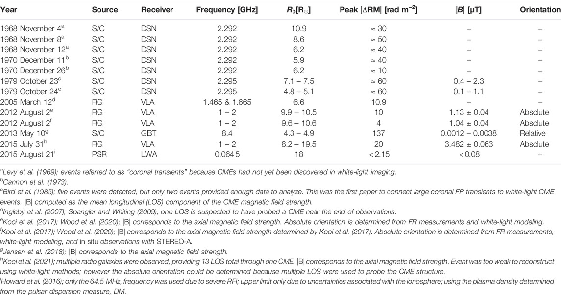
TABLE 3. Results from FR studies of coronal mass ejections. S/C, RG, and PSR are spacecraft, radio galaxy, and pulsar background radio sources, respectively.

5.1 Inferring CME Magnetic Field Strength From FR Observations

Most historical observations of CME FR utilized spacecraft as the background linearly polarized radio source because spacecraft provide strong, reliable signals with known properties; consequently, it was straightforward to rule out systematic effects that might appear as a “transient” signal in early coronal FR experiments. These early experiments (e.g. Levy et al., 1969; Cannon et al., 1973; Bird et al., 1985) are discussed in Pätzold and Bird (1998), Jensen and Russell (2008), and Kooi et al. (2017), Kooi et al. (2021). As Table 3 demonstrates, there was a sizeable gap between the 1979 observations reported in Bird et al. (1985) and the next suspected observation of CME FR in 2005. During this period, there were major developments in ground-based radio interferometry (e.g. creation and development of the VLA), improvements to computational techniques for modeling CMEs and their flux rope structure, and new generations of white-light coronagraph imagers (e.g. onboard SOHO and STEREO spacecraft). However, during this period, there was an increasingly heavy reliance on circularly polarized transmitters for communications with spacecraft; consequently, the 2000s not only marked a new era in understanding CMEs and detecting FR, but also marked the beginning of an era relying heavily on natural radio sources as the background linearly polarized pilot light.

The first CME FR observation using a natural radio source was serendipitous in nature: while performing a coronal FR observing campaign with the VLA at dual frequencies of 1465 and 1665 MHz, the outer loop of a CME approached LOS to two extragalactic radio sources (J2335–015 and J2337-025: Ingleby et al., 2007; Spangler and Whiting, 2009). Coronagraph images from LASCO-C2 suggested that the outer loop did not quite cross these LOS; however, the FR for one of the two sources (J2337-025) monotonically increased with time near the end of the observing session: increasing by $\approx 26$° (RM ≈ 10.9 rad m⁻²). Spangler and Whiting (2009) concluded there must be an MHD precursor associated with the CME ahead of the outer loop (e.g. shock or sheath region).

The first successful campaign to definitively detect CME FR using natural radio sources was reported in Kooi et al. (2017). This was the first observational campaign to use the recently upgraded VLA to hunt for CME FR. Kooi et al. (2017) used a constellation of radio galaxies surrounding the Sun, hoping to improve the likelihood that at least one LOS would probe an emerging CME. On 2012 August 2, three LOS were occulted by CMEs erupting in quick succession from the Sun; two of the CMEs produced well-defined FR profiles, ranging in values of +3 to −10 rad m⁻² at a heliocentric distance of $\approx 10{\mathrm{R}}_{\odot }$. Kooi et al. (2017) modeled these two events using a constant density force-free magnetic flux rope model and, using simultaneous white-light coronagraph measurements of TSB (see Section 3.2), calculated plasma densities of 6.9 – 21.4 × 10⁹ m⁻³ and axial magnetic field strengths of $\approx 1\mu$T.

Figure 6 shows the TSB and FR time series for a radio double that provided two closely-spaced LOS (Hot Spots 1 and 2). Near the start of the observations, the only contribution to the TSB and FR was the quiescent corona, then the leading edge of a CME (LE-1) crossed the LOS at 15:42 UT. Kooi et al. (2017) modeled the TSB and FR assuming that two CMEs occulted the source, with the leading edge of the second CME’s flux rope (LE-2) crossing the LOS near 18:30 UT. The dotted, dashed, and dash-dotted lines represent the coronal contribution, the first CME’s contribution, and the second CME’s contribution, respectively. While Kooi et al. (2017) could infer n_e and the axial field strength, they could only determine the CME’s helicity relative to the axial field direction; they could not determine the absolute geometric orientation. This was done later by Wood et al. (2020) and will be discussed further in the next section.

FIGURE 6

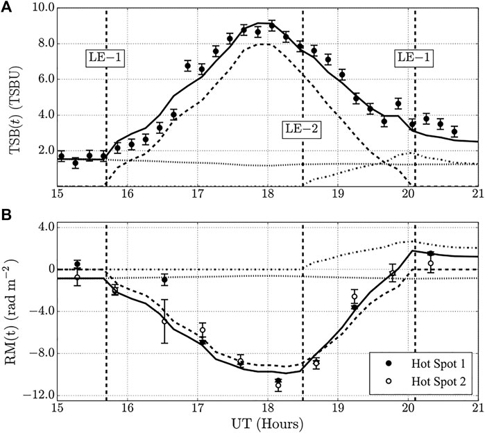
FIGURE 6. Thomson-scattering brightness (TSB, (A)) and Faraday rotation measure (RM, (B)) through CMEs using a radio galaxy as the background radio source, as reported in Kooi et al. (2017). The 2012 August 2 event was modeled assuming occultation by two CMEs; LE-1 is the leading edge of the first CME and LE-2 is the leading edge of the second. LE-1 at 15:42 UT and 20:06 UT mark the beginning and ending of occultation by the first CME, respectively. The dotted, dashed, and dash-dotted lines represent the coronal contribution, the first CME’s contribution, and the second CME’s contribution, respectively. The solid black line gives the combined effect. The radio source provided two closely-spaced LOS labeled as Hot Spots 1 and 2. These data correspond to values reported for 2012 Aug. 2^e,f in Table 3. This appears as Figure 10 in Kooi et al. (2017), ©Springer, reproduced with permission.

The only modern observation of CME FR using a spacecraft as the background transmitter was reported in Jensen et al. (2018): the LOS to the MESSENGER spacecraft was occulted by a CME on 2013 May 10. These observations were unique for three reasons. First, the downlink signal from MESSENGER is strongly circularly polarized; panel A in Figure 7 shows the fractional circular polarization prior to occultation by the CME is ≳ 99%; consequently, unlike the era of the Pioneer and Helios missions, detecting this spacecraft’s signal is like detecting a $\approx 10\%$ linearly polarized natural radio source. As panel B shows, though, the GBT was sensitive enough to accurately measure the relatively small linear polarized signal. The second important aspect of this study is that it was the first to use the apparent-Doppler tracking method in Jensen et al. (2016) to determine the change in total electron content (ΔTEC, Figure 7D) to estimate n_e inside the CME.

FIGURE 7

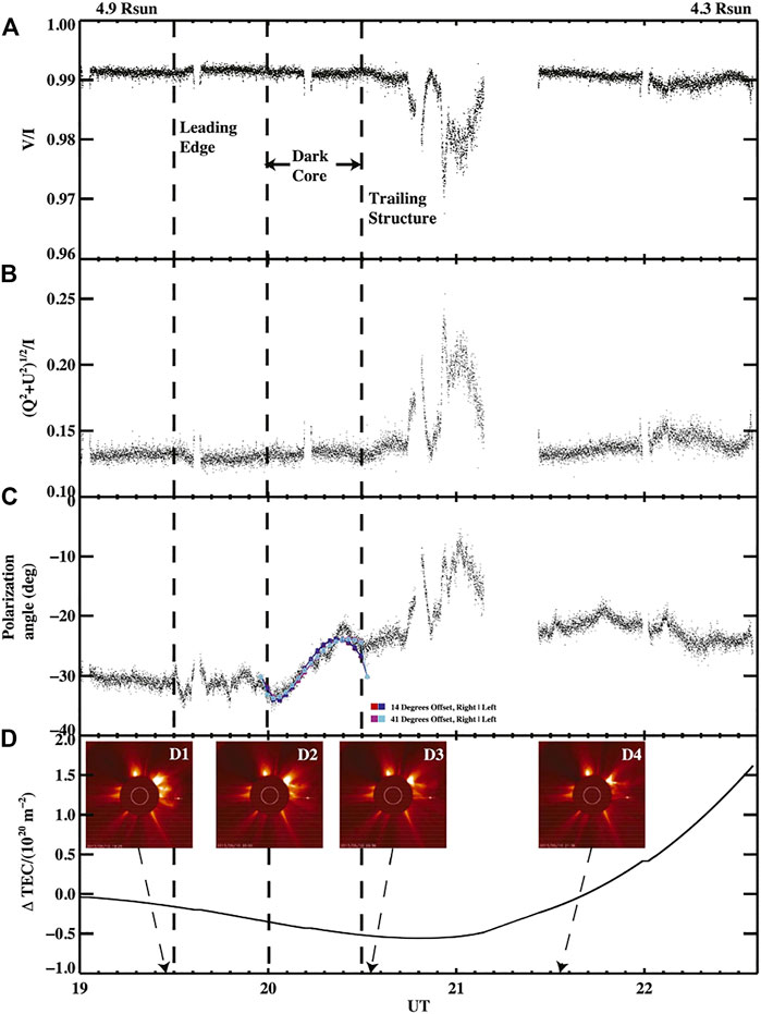
FIGURE 7. Observations of CME FR using a spacecraft as the background radio source. Panels (A) and (B) are the fractional circular and linear polarizations of the MESSENGER signal, respectively; panel (C) is the polarization angle showing the FR, with force-free magnetic flux rope fits to the “Dark Core” are overlaid in color; panel (D) is the change in TEC as determined from the apparent-Doppler tracking method (Section 3.3). White-light images from SOHO LASCO-C2 at the time periods shown are provided. Range in R₀ is shown at the top. These data correspond to values reported for 2013 May 10^g in Table 3. This appears as Figure 2 in Jensen et al. (2018), ©AAS, reproduced with permission.

Finally, while these observations did detect a characteristic flux rope profile associated with the dark inner core of the CME and infer a magnetic field strength for the axial field, they also detected a complex radio response coinciding with the trailing structure behind the flux rope. The circular polarization decreases during this period, with a corresponding increase in linear polarization that suggests mode conversion between the two was occurring. The polarization angle also experienced significant rotation during this period, similar in scale to the FR due to the flux rope structure. After eliminating receiving system bias due to spontaneous events (e.g radio bursts), Jensen et al. (2018) demonstrated that a reconnection region could reproduce these effects through an increase of the energy of the propagating LCP wave mode and, therefore, concluded that this never before seen behavior was likely due to plasma mode conversion as a result of reconnection behind the CME.

Currently, there is only one published detection of CME FR using pulsars as a background radio source. Howard et al. (2016) detected a relatively weak CME FR signal, observing pulsar PSR B0950 + 08 with the Long Wavelength Array (LWA-1: Taylor et al., 2012). They derived values for the CME n_e using both the DM and TSB (the top and middle panels of Figure 8, respectively); the cadence of white-light measurements is greater (four per hour instead of one), but the DM provides a much more sensitive measurement of the CME’s n_e structure. Unfortunately, as much as $\approx 50\%$ of the FR signal was ionospheric in origin; therefore, Howard et al. (2016) only calculated upper limits for the magnetic field strength along the LOS and did not attempt to model the CME plasma structure. The value reported in Table 3 (2015 August 21ⁱ) corresponds to the upper limit for |B| inferred using the n_e determined with the DM.

FIGURE 8

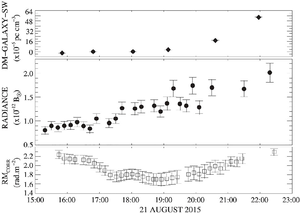
FIGURE 8. Observations of CME FR using a pulsar. Top, middle, and bottom panels give the dispersion measure (DM), radiance (i.e. TSB), and FR, respectively, due strictly to the corona and CME. At these heliocentric distances $(\approx 18{\mathrm{R}}_{\odot })$, the coronal DM is a factor of $\approx 10^4$ smaller than the interstellar DM and the coronal RM is comparable to the ionospheric RM. These data correspond to values reported for 2015 August 21ⁱ in Table 3. This appears as Figure 7 in Howard et al. (2016), ©AAS, reproduced with permission.

5.2 FR Measurements of CME Magnetic Field Orientation

A critical step towards using FR studies to enhance our understanding of space weather and, eventually, improve space weather forecasting is determining the absolute geometric orientation of CMEs (in particular, its orientation with respect to Earth’s magnetic field). It has only been within the last few years that CME FR experiments have been able to achieve this. Wood et al. (2020) was the first study to use FR to determine the absolute orientation of CMEs. Wood et al. (2020) used white-light coronagraph data from SOHO, STEREO-A, and STEREO-B to reconstruct the three-dimensional structure for two CME events discussed in Kooi et al. (2017). The left panel of Figure 9 shows the reconstruction of the two CMEs on 2012 August 2 and their positions in relation to LOS to background radio sources represented by the red and orange arrows. The blue arrow shows the line from the Sun to STEREO-A which was impacted by the northernmost CME, providing the first-ever event in which a CME’s properties could be constrained by white-light coronagraph observations, in situ spacecraft measurements, and radio FR observations.

FIGURE 9

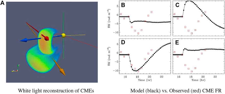
FIGURE 9. Reconstructed 3D magnetic flux rope structures of two CMEs that erupted off the western limb of the Sun given in heliocentric Earth ecliptic (HEE) coordinates (A) and the model FR (black data) for the four possible magnetic field orientations corresponding to the southern CME in panels (B–E). The blue arrow points from the Sun in the direction of STEREO-A, which was impacted by the northern CME. The red and orange arrows point from the Earth in the direction of background radio sources used in FR observations reported in Kooi et al. (2017). The axes are color-coded to match the HEE coordinate axes in the bottom-left corner. In panels (B–E), the FR measurements (red data) clearly favor the magnetic field orientation in (D). The left panel and right panels appear as Figures 4, 10, respectively, in Wood et al. (2020), ©AAS, reproduced with permission.

The southern CME was constrained using only the stereoscopic imaging and FR data. The stereoscopic imaging provided the necessary orientation information for this CME. Applying the elliptic-cylindrical analytical flux rope model from Nieves-Chinchilla et al. (2018), Wood et al. (2020) narrowed down the magnetic field orientation to four possibilities (i.e. two potential orientations for each of the axial and azimuthal field components). The FR data reported in Kooi et al. (2017) was then used to identify the correct magnetic orientation and magnitude. The right panel in Figure 9 shows the four potential orientations given the white-light geometry of this CME, similar to Figure 4. In this case, orientation (D) provides the best match to the FR data. The n_e and magnetic field strength determined from this white-light reconstruction was within a factor of 2–3 of the values reported by Kooi et al. (2017).

Kooi et al. (2021) presented the first study to determine the CME magnetic field strength and orientation using multiple LOS. These were also the first observations to utilize the VLA’s “triggered” observing mode to remotely probe CMEs. The advantage of the triggered observing mode is that one can observe a constellation of natural radio sources with LOS certain to probe the triggering CME event. Triggering observations at the sudden appearance of a CME is the only way to guarantee there are multiple LOS probing different regions of the CME.

Applying the frozen-in flux theorem, Kooi et al. (2021) scaled the n_e and axial magnetic field strength and performed a fit to the TSB and FR data across all LOS simultaneously. Figure 10 shows the TSB (A) and FR (B) for one of the sources occulted by two legs of the CME, along with the model fits. This CME was very weak in white-light images and, therefore, it was impossible to generate a reliable white-light reconstruction for this event. The CME’s boundaries (i.e. leading edges) could be determined through white-light difference imaging, though, and so the relative positions of the LOS with respect to the CME’s structure could still be determined. Kooi et al. (2021) tested three n_e models for the CME: constant density, thin shell, and thick shell (the black solid, red solid, and red dashed lines, respectively, in Figure 10). The constant density and thin shell models performed equally well and provided better fits to the data than the thick shell model, which tended to underpredict the magnitude of the FR response.

FIGURE 10

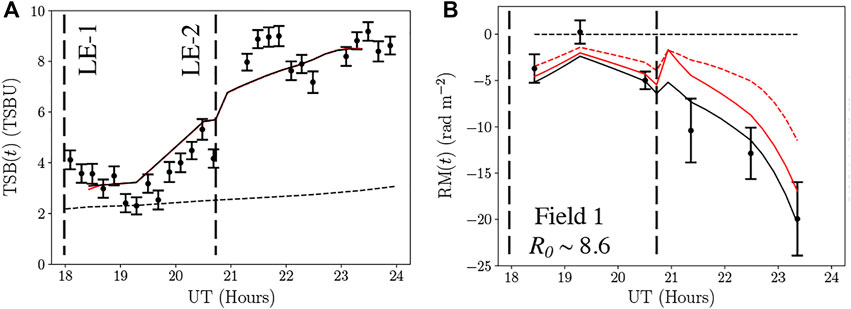
FIGURE 10. Thomson-scattering brightness (TSB, (A)) and Faraday rotation measure (RM, (B)) through a CME using a radio galaxy as the background radio source, as reported in Kooi et al. (2021). These data correspond to one of the thirteen LOS used to probe this CME. The 2015 July 31 event was modeled assuming one CME: LE-1 corresponds to the leading edge of the CME’s northern (in heliographic latitude) leg and LE-2 corresponds to the leading edge of the southern leg. The black dashed line corresponds to the coronal contribution. The black solid, red solid, and red dashed lines correspond to the constant density, thin shell, and thick shell CME n_e models. These data correspond to values reported for 2015 July 31^h in Table 3. This appears as Figure 9 in Kooi et al. (2021), ©Springer, reproduced with permission.

Kooi et al. (2021) is a good example of the power of multiple LOS and is indicative of the potential for multi-LOS observations using current and future observatories that can image large regions of the sky. In just under a decade, CME FR observations have gone from one LOS to 10+; future ground-based instruments will soon open up the ability to image 10s, 100s, and eventually, 1000s of LOS. Even with one LOS, Kooi et al. (2017) and Wood et al. (2020) together showcase the promise of combining white-light reconstructions of CME morphology with radio FR observations.

These studies of CMEs erupting on or near the solar limb also set the stage for future observations of Earth-directed CMEs. The next major step towards using Faraday rotation as a space weather forecasting method is demonstrating that Faraday rotation can retrieve the magnetic field orientation of these Earth-directed CMEs. Modern radio interferometers such as the VLA can reach the necessary sensitivities (typically a few 10s μJy beam⁻¹ for radio galaxies with linear polarization intensities P > 5 mJy beam⁻¹, e.g. see Kooi et al., 2021) within minutes; consequently, future facilities could potentially generate sky maps similar to those simulated in Figure 4 every few minutes or faster, especially with further development of automated polarization calibration data reduction pipelines.

6 The Future of Coronal Faraday Rotation Studies

Taken together, the studies presented in this review provide a promising look ahead at what might soon be accomplished with the next generation of FR experiments. In this section, we discuss current and future instruments and methods that will benefit and, in turn, be enhanced by FR studies.

6.1 Opportunities for Improvement in Ground-Based FR Observations

6.1.1 The Potential for New Radio Transmitters

Fundamentally, there are two means of improving ground-based FR experiments: using better background radio sources and developing better receivers to detect radio sources. Here, we discuss the former, delineating between spacecraft and natural sources. Improving spacecraft signals to, in turn, improve prospects for future FR observations is simple: equip spacecraft with linearly polarized radio communication systems. As discussed in previous sections (e.g. Section 5.1), recent space missions have chosen circularly polarized radio transmitters to communicate with Earth. While the most sensitive telescopes can still detect residual linear polarization within these signals (e.g. the GBT, as discussed in Jensen et al., 2018), it is imperative that the next generation of spacecraft - in particular, spacecraft that will regularly be in conjunction with the Earth-Sun line - be equipped with linear transmitters if we are ever to repeat and improve upon the FR successes of, e.g., the Pioneer or Helios missions.

Further, the two biggest flaws of using spacecraft transmitters must be redressed: one or two downlink frequencies and one LOS. The former is simple to improve: equip spacecraft with multi-frequency downlink antennas, ideally broadcasting over the range of 2–12 GHz. While the frequencies could remain discrete in nature, they should be phase-locked similar to Cassini to remove systematic effects (e.g. see Jensen et al., 2016). With a range of frequencies available, such spacecraft could easily be tracked and provide sensitive FR measurements over a broad range of heliocentric distances: S-band (2–4 GHz) could be used to probe the outer corona $(>6{\mathrm{R}}_{\odot })$, C- and X-bands (4–8 and 8–12 GHz, respectively) could be used to probe the middle corona (1.5 < r < 6 R_⊙), and Ku-band and higher ($>12$ GHz) could be used to probe the inner corona $(<1.5{\mathrm{R}}_{\odot })$.

The second flaw in spacecraft transmitters is that one spacecraft provides one LOS. The remedy is similarly straightforward, though more expensive to implement: future missions should be flown using multiple spacecraft flying in formation. Monitoring these satellite constellations during conjunctions would provide the same benefits of FR observations of extended radio galaxies:

1. FR could be observed over multiple (downlink) frequencies;

2. satellite constellations would provide multiple LOS, but with the added benefit of each LOS providing a much stronger signal than those typical for radio galaxies extended on the sky;

3. satellite constellations would provide multiple, closely-spaced LOS to detect electric currents using DFR methods (Section 4.2).

Constellations of multi-frequency satellites with linearly polarized transmitters could also be tracked by simpler radio telescopes or telescope networks like the NASA Deep Space Network (DSN) on a regular basis. As Table 3 demonstrates, most modern observations of, e.g., CME FR have to be done with extremely powerful, specialized radio telescopes or interferometers, such as the VLA or GBT. These are very competitive, PI-driven instruments and are, therefore, best used to test new methods for FR observations; they are not designed to be solar observatories. Satellite clusters such as this would allow us to move towards ground-based tracking of coronal FR on a daily or near-daily basis, similar to what was done during the Helios mission decades ago.

Daily FR observations using a satellite swarm combined with rapid white-light reconstruction methods could be used in a similar fashion to Wood et al. (2020), returning the absolute orientation of CMEs bound for Earth; this would be an important step forward for space weather forecasting. Similarly, the sensitive measurements of reconnection behind the CME observed by Jensen et al. (2018) offer a tantalizing preview of the new science that could be explored combining FR campaigns with satellites transmitting at multiple frequencies.

Satellite swarms would not entirely replace the role of natural radio sources. A number of current and future radio telescopes are designed to image large regions of the sky (e.g. the MWA, a precursor instrument to the Square Kilometre Array, SKA, has a field of view of hundreds of square degrees). While there are important challenges to overcome, chief among them understanding the instrument’s polarization properties and mitigating ionospheric effects on these scales, these instruments will likely be able to take full advantage of the natural linearly polarized emitters on the sky. There are hundreds of suitable natural radio sources within, e.g., 20 R_⊙ of the Sun on any given day; consequently, these instruments should one day be able to generate FR maps of the corona or CMEs, using sparse tomography methods perhaps, similar to the MWA maps simulated by Jensen et al. (2010). Once FR tomography methods can be realized, more advanced methods to distinguish between n_e and B_∥ contributions will be required. There are already new methods being developed to provide time-dependent, three-dimensional reconstructions of the solar wind using observations of coronal Thomson scattering or interplanetary scintillation (see Jackson et al., 2020, and references therein).

Soon, there will likely be even more natural radio sources deemed suitable for coronal FR experiments. Natural radio sources are identified and selected based on their known polarization properties, which are usually determined from data collected during sky surveys. For instance, most of the radio galaxies used in coronal FR experiments with the VLA are sources studied as part of the NRAO VLA Sky Survey (NVSS: Condon et al., 1998), performed at 1.4 GHz and covering the sky north of a declination of −40°. The recently upgraded VLA is currently performing a new survey, the VLA Sky Survey (VLASS: Lacy et al., 2020), at frequencies of 2–4 GHz, again covering the whole sky visible to the VLA. The survey is being performed across three epochs; the first observations began in September 2017, and the last observations will finish in 2024. Further, the VLA Low-band Ionosphere and Transient Experiment (VLITE: Polisensky et al., 2016; Helmboldt et al., 2019) is operating as a commensal system on 18 of the 27 VLA antennas, providing simultaneous observations at 320–384 MHz as part of the VLA Commensal Sky Survey (VCSS). Both VLASS and VCSS will provide a wealth of new data and, potentially, a wealth of new sources at these frequencies.

6.1.2 Improvements in Ground-Based Receivers

In the past two decades, the hardware for older radio telescopes have been significantly upgraded. The VLA, which was formally dedicated in 1980, was recently upgraded through the Expanded VLA (EVLA) project and renamed the Karl G. Jansky Very Large Array in 2012. As a result, the maximum instantaneous bandwidth and the continuum sensitivity have improved by factors of 80 and 10, respectively. Most solar FR observations with the VLA have been made using the L-, S-, and C-band receivers. Historical VLA observations (i.e. prior to 2012) were restricted to two simultaneous observing frequencies; however, since the upgrade, the VLA is now capable of providing the full 1–2 GHz at L-band, the full 2–4 GHz at S-band, and the full 4–8 GHz at C-band.

Within the next two decades, two new major radio telescopes are expected to become operational: the Square Kilometre Array and the Next Generation Very Large Array. The Square Kilometre Array⁴ (SKA), will eventually use thousands of dishes and up to a million low-frequency antennas, co-hosted across two continents: South Africa’s Karoo region will host the core of the high and mid frequency dishes (SKA-mid) and Australia’s Murchison Shire will host the low-frequency antennas (SKA-low). The system will be built across two phases. At the end of phase 1, the low-frequency SKA1-low will cover frequencies of 50 − 350 MHz using ≈131,000 antennas spread across 512 stations and the mid-frequency SKA1-mid will cover frequencies of 350 MHz to 15.3 GHz using 197 dishes. Together, SKA-low and SKA-mid will provide an unprecedented view of the southern radio sky.

The Next Generation Very Large Array⁵ (ngVLA) is a similarly ambitious project to deploy radio dishes across the United States of America, Puerto Rico, the U.S. Virgin Islands, Canada, and northern Mexico, observing at frequencies of $\approx 1.2-116$ GHz. Unlike the current VLA, the ngVLA will not be reconfigurable; instead, the ngVLA will consist of three fundamental subarrays: the Main Interferometric Array consisting of 214 antennas 18 m in diameter, the Short Baseline Array (SBA) consisting of 19 antennas 6 m in diameter, and the Long Baseline Array (LBA) consisting of 30 antennas, again, 18 m in diameter. In principle, the ngVLA can be operated in combinations of these subarrays or subsets of these subarrays depending on the science goals. The SKA and ngVLA are scheduled to begin routine science operations in the late 2020s and mid-2030s, respectively. While neither instrument is designed to be a solar telescope, they will be crucial to developing the future generation of radio remote-sensing methods (e.g. see Bastian, 2018), much as the GBT and VLA have been used in recent years to develop and test methods such as apparent-Doppler tracking and DFR.

6.2 Coordinating FR Campaigns With Current and Future Missions

As an integrated LOS measurement that depends on the product of n_e and B_∥ along the LOS, improvements in our ability to assess the n_e contribution will similarly provide improvements in our ability to infer magnetic field structure from FR observations. While future implementation of satellite swarms with multi-frequency linearly polarized transmitters for solar missions will no doubt improve our understanding of the n_e for satellite-based FR programs (e.g. using ranging and apparent-Doppler tracking methods, Section 3.3), future studies using natural background sources will require alternative methods. Section 3.2 discussed the application of white-light coronagraph TSB data from the SOHO LASCO and STEREO SECCHI instruments to previous FR studies. Newer spacecraft-borne suites such as the Wide-field Imager for Solar PRobe (WISPR: Vourlidas et al., 2016) onboard the Parker Solar Probe (PSP: Fox et al., 2016) and the upcoming Polarimeter to Unify the Corona and Heliosphere⁶ (PUNCH, PI: Craig DeForest) mission have the potential to advance current techniques to determine n_e in FR studies.

WISPR provides a unique opportunity for enhanced understanding of coronal plasma in FR studies. By itself, WISPR’s inner telescope could provide insights into the morphology of the plasma structures upstream from radio LOS probing the coronal plasma. Future FR studies, though, should strive to develop methods of running LOS through the WISPR field-of-view in order to gain more detailed information about the specific density enhancements along the LOS. WISPR has so far provided an unparalleled view of coronal phenomena such as CMEs, substreamers, or even magnetic islands (Howard et al., 2019); using WISPR to understand the density variations these structures introduce to complementary FR observations will dramatically improve FR studies of magnetic field fluctuations.

PSP’s rapid orbital speed, particularly near each perihelion, creates the potential for a novel science capability: detailed tomographic reconstruction of the corona in the vicinity of the spacecraft. In consecutive WISPR images near perihelion, the relative motion of the spacecraft (with respect to the coronal features that WISPR images) produce perspective changes which dominate scene changes. If WISPR tomography research progresses to the point that near-perihelion datasets can yield inversions of the K corona, then we can leverage these coronal reconstructions to obtain detailed information on density enhancements local to PSP and gain insight on plasma structures that occulted the LOS. For these reasons, we recommend future observing campaigns using, e.g., the GBT or VLA should be coordinated with PSP perihelion events. WISPR can provide contextual data for ground-based FR observations of the solar wind and, in turn, FR observations can provide contextual data on the large-scale magnetic structures that are measured in situ by the FIELDS instrument onboard PSP (Bale et al., 2016).

The upcoming NASA small explorer mission PUNCH, scheduled to launch in 2023, will observe both visible light and its linear polarization using four satellites whose single coronagraph and three wide-field imagers will remain in Sun-synchronous, low-Earth orbit. PUNCH seeks to understand the evolution of coronal structures into solar wind and the evolution of young, transient solar wind features themselves. The sensitivity of the imagers to polarized brightness will enable 3D localization of solar wind features. Future FR experiments should leverage this 3D information on heliospheric structures to gain a deeper understanding of the features probed by the LOS. PUNCH is designed to image the corona-to-wind transition region, 6–80 R_⊙, every 4 minutes and will provide mosaic images of the corona out to 180 R_⊙ three times per orbit. This is a factor of three improvement in cadence over, e.g., LASCO, which has been used in recent FR studies discussed in this paper. Observations such as Howard et al. (2016) and Kooi et al. (2017, 2021) have laid a foundation for implementing coronagraph data into FR studies; expanding these methods to include data from the PUNCH mission will likely revolutionize the white-light component of coronal FR investigations using extragalactic radio sources.

6.3 Implementing FR Capabilities in Future Space Missions

The concept of building FR capabilities into future space missions has been around for at least a few decades. Pätzold et al. (1995) proposed the Solar Corona Sounders (SCS) mission consisting of two spacecraft located near Lagrange point L3, transmitting at 2.3 GHz and 8.4 GHz for continuous radio sounding of the corona. The orbits they proposed would provide two LOS with solar impact parameters 3–5 R_⊙ and 10–13 R_⊙. However, coronal FR missions that rely on ground-based receivers will always be severely limited by the Earth’s ionosphere.

The ionosphere is another magnetized medium through which the radio signal propagates en route to ground-based receiving telescopes. As a result, the ionosphere introduces direction- and time-dependent effects over a range of physical (≲ 100 km to ≳ 1000 km) and temporal (≲ min to ≳ hour) scales. These effects produce, among other things, an ionospheric phase delay (∝ ν⁻¹) and ionospheric FR, which is typically within the range of 2–6 rad m⁻² at mid-latitudes (Oberoi and Lonsdale, 2012); consequently, at heliocentric distances ≳ 20 R_⊙ the magnitude of ionospheric FR becomes comparable, if not larger than typical values of coronal FR. Further complicating matters are the fluctuations in ionospheric FR, which can be misinterpreted as coronal fluctuations. For these reasons, accurate ionospheric mitigation techniques are critical to coronal FR observations. While there are many methods for modeling or mitigating ionospheric effects, the simplest way to remove this restriction is to observe coronal FR using receivers located on spacecraft well outside the Earth’s ionosphere.

An instructive example is the Multiview Observatory for Solar Terestrial science mission concept (MOST: Gopalswamy et al., 2021a). The primary goal of MOST is to understand the magnetic coupling between the solar interior and the heliosphere. The mission concept includes four spacecraft: two large spacecraft deployed at Sun-Earth Lagrange points L4 and L5 and two smaller spacecraft, one ahead of L4 and the other behind L5. These large spacecraft will host a suite of ten instruments, seven remote-sensing and three in situ instruments, to provide wide-ranging imagery and time series data to improve understanding of the solar drivers and the heliospheric responses as a system, as well as identify and track 3D magnetic field structures (both transient and quiescent) in the inner heliosphere (Gopalswamy et al., 2021a). The suite of instruments will include:

1. Magnetic and Doppler Imager (MaDI) to investigate surface and subsurface magnetism by exploiting the combination of helioseismic and magnetic-field measurements in the photosphere;

2. Inner Coronal Imager in EUV (ICIE) to study large-scale structures such as active regions, coronal holes and eruptive structures by capturing the magnetic connection between the photosphere and the corona to $\approx 3{\mathrm{R}}_{\odot }$;

3. Hard X-ray Imager (HXI) to image the non-thermal flare structure;

4. White-light Coronagraph (WCOR) to seamlessly study transient and quiescent large-scale coronal structures extending from the ICIE field of view;

5. Faraday Effect Tracker of Coronal and Heliospheric structures (FETCH), hosted on all four spacecraft, is a novel radio package to determine the magnetic field structure and plasma column density, and their evolution within 0.5 AU;

6. Heliospheric Imager with Polarization (HIP) to track solar features beyond the WCOR field of view, study their impact on Earth, and provide important context for FETCH;

7. Radio and Plasma Wave instrument (M/WAVES) to study electron beams and shocks propagating into the heliosphere via passive radio emission;

8. Solar High-energy Ion Velocity Analyzer (SHIVA) to determine spectra of electrons, and ions from H to Fe at multiple spatial locations and use energetic particles as tracers of magnetic connectivity;

9. Solar Wind Magnetometer (MAG) to characterize magnetic structures at 1 AU;

10. Solar Wind Plasma Instrument (SWPI) to characterize plasma structures at 1 AU.

Of these instruments, FETCH will, for the first time, perform spacecraft-to-spacecraft FR measurements of the solar wind. FETCH will consist of four transmitter/receiver instruments onboard the four MOST spacecraft. The four LOS provided by the four spacecraft will enable space-based FR studies to probe magnetic field structure and CME evolution at solar impact parameters $<0.5\mathrm{A}\mathrm{U}$. Cummer et al. (2001, 2003), Zhai and Cummer (2006), and Zhai et al. (2011) successfully demonstrated the first spacecraft-to-spacecraft FR using the Radio Plasma Imager instrument (RPI; Reinisch et al., 2000) onboard the Imager for Magnetopause-to-Aurora Global Exploration (IMAGE; Burch, 2000) as the transmitter and the WAVES instrument (Bougeret et al., 1995) onboard Wind as the receiver. They measured FR through the Earth’s magnetosphere over distances of $\le 15{\mathrm{R}}_{\mathrm{E}}$ (≈ 95,700 km). The distance between MOST spacecraft will be $\approx 2\mathrm{A}\mathrm{U}$ ($\approx 300$ million km), which is three orders of magnitude greater than the IMAGE-Wind experiment LOS.

Because FETCH will return FR data for solar wind plasma upstream from both the Earth and satellites orbiting L1, FETCH has the potential to enhance space weather forecasting capabilities (Jensen et al., 2021). FETCH will also provide unique insights into solar wind phenomena such as stream interaction regions or co-rotating interaction regions (Wexler et al., 2021b). 2D FR analysis will be possible with the FETCH configuration: plasma parcels sampled on any particular path are discretely different from each other; consequently, signals sent to/from the same spacecraft simultaneously, due to light time delay (e.g., $\approx 12$ minutes between L4 and L5), pass through different plasma structures. Wood et al. (2020) showcases the power of combining white light morphological imaging, in situ measurements, and FR observations to better understand CME structures with even one radio LOS. FETCH’s four LOS combined with imagers such as HIP and WCOR will likely revolutionize our understanding of the solar wind plasma upstream from Earth.

6.4 Enhancing FR Observations Through Machine Learning

Machine learning (ML) algorithms provide a method for training computers to detect patterns, classify data, make predictions, or simulate new data (Fluke and Jacobs, 2020). The two main categories of ML are supervised learning and unsupervised learning. Supervised ML algorithms determine a mapping between input (e.g. a set of features) and output (e.g. a target variable) using training examples (Baron, 2019). The supervisor providing the input-output example oversees the learning process by providing “labels” for the data, but not an a priori model for the data; model generation is the task of the ML algorithm. Unsupervised algorithms learn complex relationships without the need for labels or examples and, thus, without any guidance from a supervisor.

Within solar astronomy, ML has been used to classify solar flares, CME productivity, and photospheric features as well as CME arrival time prediction (e.g. the supervised Support Vector Machine, SVM, Algorithm: Liu et al., 2018). ML constitutes a vast and deep reservoir of tools to detect inconspicuous relationships in data sets, provide new insights, generate and adapt models, and predict and forecast outcomes for new observational data. Supervised ML algorithms would greatly enhance FR studies of CMEs. As Figure 3 demonstrates, different orientations of the CME flux rope produce a wide variety of FR profiles; consequently, one of the most challenging aspects of interpreting CME FR profiles is determining the correct orientation.

Two subdivisions within supervised learning - classification and regression - should be explored to determine which is best suited to determining CME orientation. Classification learning assigns discrete labels or classes to objects in the data using a training set; the algorithm identifies correlation between the objects and classes and then assigns new data to the most likely category. In this case, different classes would represent different flux rope orientations. Regression learning exhibits many similar traits to classification; the difference lies in the assignment. While classification sorts objects into classes, regression assigns continuous numerical values to each object (Baron, 2019). In this case, regression methods could be trained to assign cone and clock angles (see Jensen et al., 2010, for details) based on FR profiles. For future missions like MOST, a combination of white light morphology and ML enhanced FR analysis could potentially rapidly determine the orientation of CMEs upstream from Earth, before impact. This would be a powerful new tool for space weather forecasting.

7 Summary

Faraday rotation is a proven method for characterizing the magnetic field strength and structure of the corona and, over the last decade, has developed into a powerful tool for probing the plasma structure of CMEs. FR observations are versatile: they can be used to understand the large-scale coronal magnetic field, measure magnetic field fluctuations, and detect electric currents. In the last two decades, the sensitivity of magnetic field measurements using FR have been enhanced by the development of new methods to provide independent information for n_e: application of the dispersion measure for background pulsars; implementation of coronagraph Thomson scattering brightness measurements for background radio galaxies; and radio ranging and apparent-Doppler tracking for background spacecraft. FR methods are now at the stage where they can be used to probe reconnection events trailing behind CMEs and, critical to space weather applications, determine the absolute orientation of a CME’s magnetic field, by using multiple lines of sight or combining FR observations with white light imaging methods and in situ measurements. Future solar missions involving satellite swarms should be designed with linearly polarized spacecraft transmitters for complementary ground-based FR observations or should directly incorporate spacecraft-to-spacecraft FR measurements in their mission design (e.g. MOST).

Author Contributions

JK was responsible for the organization of this article and contributed to all sections. DW was also responsible for the article’s organization and made major contributions to Sections 1, 2, 4, and 6. EJ also made major contributions to Sections 1, 3, 5, and 6. MK made major contributions to Sections 1, 2, and 6. TC and BW made contributions to Sections 5 and 6. LW, LJ, SF, NG, and WM made contributions to Sections 1 and 6. AP made contributions to Sections 2 and 6.

Funding

Basic research at the U.S. Naval Research Laboratory (NRL) is supported by 6.1 base funding. The National Solar Observatory (NSO) is operated by the Association of Universities for Research in Astronomy (AURA), Inc., under cooperative agreement with the National Science Foundation.

Conflict of Interest

The authors declare that the research was conducted in the absence of any commercial or financial relationships that could be construed as a potential conflict of interest.

Publisher’s Note

All claims expressed in this article are solely those of the authors and do not necessarily represent those of their affiliated organizations, or those of the publisher, the editors and the reviewers. Any product that may be evaluated in this article, or claim that may be made by its manufacturer, is not guaranteed or endorsed by the publisher.

Acknowledgments

The authors wish to thank the MOST FETCH team for providing useful feedback concerning the topics and ideas presented in this paper. The authors are also grateful for the time and effort both reviewers put into this article. Their thorough reviews and insights greatly improved the presentation and clarity of this work.

Footnotes

¹Details can be found at wso.stanford.edu

²https://gong2.nso.edu/products/mainView/table.php?configFile=configs/mainView.cfg

³https://naif.jpl.nasa.gov/naif/spiceconcept.html

⁴https://www.skatelescope.org/

⁵https://ngvla.nrao.edu/

⁶https://punch.spaceops.swri.org/

References

Allen, C. W. (1947). Interpretation of Electron Densities from Corona Brightness. Monthly Notices R. Astronomical Soc. 107, 426–432. doi:10.1093/mnras/107.5-6.426

CrossRef Full Text | Google Scholar

Andreev, V. E., Efimov, A. I., Samoznaev, L. N., Chashei, I. V., and Bird, M. K. (1997). Characteristics of Coronal Alfven Waves Deduced from HELIOS Faraday Rotation Measurements. Solar Phys. 176, 387–402. doi:10.1023/A:1004965310604

CrossRef Full Text | Google Scholar

Badman, S. T., Bale, S. D., Rouillard, A. P., Bowen, T. A., Bonnell, J. W., Goetz, K., et al. (2021). Measurement of the Open Magnetic Flux in the Inner Heliosphere Down to 0.13 AU. Astron. Astrophys. 650, A18. doi:10.1051/0004-6361/202039407

CrossRef Full Text | Google Scholar

Bale, S. D., Goetz, K., Harvey, P. R., Turin, P., Bonnell, J. W., Dudok de Wit, T., et al. (2016). The FIELDS Instrument Suite for Solar Probe Plus. Space Sci. Rev. 204, 49–82. doi:10.1007/s11214-016-0244-5

PubMed Abstract | CrossRef Full Text | Google Scholar

Banaszkiewicz, M., Axford, W. I., and McKenzie, J. F. (1998). An Analytic Solar Magnetic Field Model. Astron. Astrophys. 337, 940.

Google Scholar

Baron, D. (2019). Machine Learning in Astronomy: a Practical Overview. arXiv e-prints, arXiv:1904.07248. doi:10.48550/arXiv.1904.07248

CrossRef Full Text | Google Scholar

Bastian, T. S. (2018). “ngVLA Observations of the Solar Wind,” in Science with a Next Generation Very Large Array. Editor E. Murphy (San Francisco: 517 of Astronomical Society of the Pacific Conference Series), 87.

Google Scholar

Bastian, T. S., Pick, M., Kerdraon, A., Maia, D., and Vourlidas, A. (2001). The Coronal Mass Ejection of 1998 April 20: Direct Imaging at Radio Wavelengths. Astrophys. J. Lett. 558, L65–L69. doi:10.1086/323421

CrossRef Full Text | Google Scholar

Bird, M. K. (2007). Coronal Faraday Rotation of Occulted Radio Signals. Astronomical Astrophysical Trans. 26, 441–453. doi:10.1080/10556790701595236

CrossRef Full Text | Google Scholar

Bird, M. K. (1982). Coronal Investigations with Occulted Spacecraft Signals. Space Sci. Rev. 33, 99–126. doi:10.1007/BF0021325010.1007/bf00213250

CrossRef Full Text | Google Scholar

Bird, M. K., and Edenhofer, P. (1990). “Remote Sensing Observations of the Solar Corona,”. Editors R. Schwenn, and E. Marsch (Berlin Heidelberg: Springer-Verlag), 13–97. doi:10.1007/978-3-642-75361-9_2

CrossRef Full Text | Google Scholar

Bird, M. K., Pätzold, M., Edenhofer, P., Asmar, S. W., and McElrath, T. P. (1996). Coronal Radio Sounding with Ulysses: Solar Wind Electron Density Near 0.1AU during the 1995 Conjunction. Astron. Astrophys. 316, 441–448.

Google Scholar

Bird, M. K., Schrüfer, E., Volland, H., and Sieber, W. (1980). Coronal Faraday Rotation during Solar Occultation of PSR0525 + 21. Natur.e 283, 459–460. doi:10.1038/283459a0

CrossRef Full Text | Google Scholar

Bird, M. K., Volland, H., Efimov, A. I., Levy, G. S., Seidel, B. L., and Stelzried, C. T. (1992). “Coronal Alfvén Waves Detected by Radio Sounding During the Solar Occultations of the Helios Spacecraft,” in Solar Wind Seven Colloquium. Editors E. Marsch, and R. Schwenn, 147–150. doi:10.1016/b978-0-08-042049-3.50032-6

CrossRef Full Text | Google Scholar

Bird, M. K., Volland, H., Howard, R. A., Koomen, M. J., Michels, D. J., and Sheeley, N. R. (1985). White Light and Radio Sounding Observations of Coronal Transients. Solar Phys. 98, 341–368. doi:10.1007/BF00152465

CrossRef Full Text | Google Scholar

Bisi, M. M., Pacini, A., Aguilar-Rodriguez, E., Tokumaru, M., Gonzalez-Esparza, A., Jackson, B., et al. (2021). “A Ground-Based Heliospheric Observatory for Space Weather: The Worldwide Interplanetary Scintillation (IPS) Stations (WIPSS) Network,” in 43rd COSPAR Scientific Assembly, 2370.43.

Google Scholar

Bougeret, J. L., Kaiser, M. L., Kellogg, P. J., Manning, R., Goetz, K., Monson, S. J., et al. (1995). Waves: The Radio and Plasma Wave Investigation on the Wind Spacecraft. Space Sci. Rev. 71, 231–263. doi:10.1007/BF00751331

CrossRef Full Text | Google Scholar

Brower, D. L., Ding, W. X., Terry, S. D., Anderson, J. K., Biewer, T. M., Chapman, B. E., et al. (2002). Measurement of the Current-Density Profile and Plasma Dynamics in the Reversed-Field Pinch. Phys. Rev. Lett. 88, 185005. doi:10.1103/physrevlett.88.185005

PubMed Abstract | CrossRef Full Text | Google Scholar

Brueckner, G. E., Howard, R. A., Koomen, M. J., Korendyke, C. M., Michels, D. J., Moses, J. D., et al. (1995). The Large Angle Spectroscopic Coronagraph (LASCO). Solar Phys. 162, 357–402. doi:10.1007/BF00733434

CrossRef Full Text | Google Scholar

Büchner, J. (2006). Locating Current Sheets in the Solar Corona. Space Sci. Rev. 122, 149–160. doi:10.1007/s11214-006-8213-z

CrossRef Full Text | Google Scholar

Burch, J. L. (2000). IMAGE mission Overview. Space Sci. Rev. 91, 1–14. doi:10.1007/978-94-011-4233-5_1

CrossRef Full Text | Google Scholar

Burlaga, L. F. (1988). Magnetic Clouds and Force-free fields with Constant Alpha. J. Geophys. Res. 93, 7217. doi:10.1029/ja093ia07p07217

CrossRef Full Text | Google Scholar

Burlaga, L., Sittler, E., Mariani, F., and Schwenn, R. (1981). Magnetic Loop behind an Interplanetary Shock - Voyager, Helios, and IMP 8 Observations. J. Geophys. Res. 86, 6673. doi:10.1029/JA086iA08p06673

CrossRef Full Text | Google Scholar

Cannon, A. R., Stelzried, C. T., and Ohlson, J. E. (1973). Faraday Rotation Observations During the 1970 Pioneer 9 Solar Occultation. Deep Space Netw. Prog. Rep. 16, 87–93.

Google Scholar

Chashei, I. V., Bird, M. K., Efimov, A. I., Andreev, V. E., and Samoznaev, L. N. (1999). Five-minute Magnetic Field Fluctuations in the Solar Wind Acceleration Region. Solar Phys. 189, 399–412. doi:10.1023/A:1005223531849

CrossRef Full Text | Google Scholar

Chashei, I. V., and Shishov, V. I. (1983). Solar Wind Turbulence in the Acceleration Region. Sov. Astron. 27, 346.

Google Scholar

Chashei, I. V., and Shishov, V. I. (1984). The Turbulence in the Solar Atmosphere and in the Interplanetary Plasma. Sov. Astron. 28, 279–284.

Google Scholar

Chashei, I. V., and Shishov, V. I. (1986). Origin of Low-Frequency Alfven Waves in the Solar Wind. Sov. Astron. 30, 322–326.

Google Scholar

Chen, J. (1996). Theory of Prominence Eruption and Propagation: Interplanetary Consequences. J. Geophys. Res. 101, 27499. doi:10.1029/96JA02644

CrossRef Full Text | Google Scholar

Condon, J. J., Cotton, W. D., Greisen, E. W., Yin, Q. F., Perley, R. A., Taylor, G. B., et al. (1998). The Nrao Vla Sky Survey. Astron. J. 115, 1693–1716. doi:10.1086/300337

CrossRef Full Text | Google Scholar

Counselman, I., Charles, C., and Shapiro, I. I. (1968). Scientific Uses of Pulsars. Science 162, 352–355. doi:10.1126/science.162.3851.352-a

PubMed Abstract | CrossRef Full Text | Google Scholar

Cranmer, S. R., van Ballegooijen, A. A., and Edgar, R. J. (2007). Self-consistent Coronal Heating and Solar Wind Acceleration from Anisotropic Magnetohydrodynamic Turbulence. Astrophys. J. Supp. 171, 520–551. doi:10.1086/518001

CrossRef Full Text | Google Scholar

Cummer, S. A., Green, J. L., Reinisch, B. W., Fung, S. F., Kaiser, M. L., Pickett, J. S., et al. (2003). Advances in Magnetospheric Radio Wave Analysis and Tomography. Adv. Space Res. 32, 329–336. doi:10.1016/S0273-1177(03)90271-7

CrossRef Full Text | Google Scholar

Cummer, S. A., Reiner, M. J., Reinisch, B. W., Kaiser, M. L., Green, J. L., Benson, R. F., et al. (2001). A Test of Magnetospheric Radio Tomographic Imaging with IMAGE and WIND. Geophys. Res. Lett. 28, 1131–1134. doi:10.1029/2000gl012683

CrossRef Full Text | Google Scholar

Ding, W. X., Brower, D. L., Terry, S. D., Craig, D., Prager, S. C., Sarff, J. S., et al. (2003). Measurement of Internal Magnetic Field Fluctuations in a Reversed-Field Pinch by Faraday Rotation. Phys. Rev. Lett. 90, 035002. doi:10.1103/PhysRevLett.90.035002

PubMed Abstract | CrossRef Full Text | Google Scholar

Domingo, V., Fleck, B., and Poland, A. I. (1995). The SOHO Mission: an Overview. Solar Phys. 162, 1–37. doi:10.1007/bf00733425

CrossRef Full Text | Google Scholar

Edenhofer, P., Lueneburg, E., Esposito, P. B., Martin, W. L., Zygielbaum, A. I., Hansen, R. T., et al. (1977). Time Delay Occultation Data of the Helios Spacecraft and Preliminary Analysis for Probing the Solar corona. J. Geophys. Z. Geophys. 42, 673–698.

Google Scholar

Efimov, A. I., Chashei, I. V., Shishov, V. I., and Bird, M. K. (1993). Faraday-rotation Fluctuations during Radio Occultation of the Circumsolar Plasma. Astron. Lett. 19, 57.

Google Scholar

Efimov, A. I., Lukanina, L. A., Rogashkova, A. I., Samoznaev, L. N., Chashei, I. V., Bird, M. K., et al. (2015a). Coronal Radio Occultation Experiments with the Helios Solar Probes: Correlation/Spectral Analysis of Faraday Rotation Fluctuations. Solar Phys. 290, 2397–2408. doi:10.1007/s11207-015-0687-y

CrossRef Full Text | Google Scholar

Efimov, A. I., Lukanina, L. A., Rogashkova, A. I., Samoznaev, L. N., Chashei, I. V., Bird, M. K., et al. (2015b). Faraday-rotation Fluctuations from Radio-Sounding Measurements of the Circumsolar Plasma Using Polarized Signals from the HELIOS-1 and HELIOS-2 Space Probes. Astron. Rep. 59, 313–326. doi:10.1134/S1063772915040022

CrossRef Full Text | Google Scholar

Efimov, A. I., Samoznaev, L. N., Andreev, V. E., Chashei, I. V., and Bird, M. K. (2000). Quasi-Harmonic Faraday-Rotation Fluctuations of Radio Waves When Sounding the Outer Solar Corona. Astron. Lett. 26, 544–552. doi:10.1134/1.1306991

CrossRef Full Text | Google Scholar

Fluke, C. J., and Jacobs, C. (2020). Surveying the Reach and Maturity of Machine Learning and Artificial Intelligence in Astronomy. WIREs Data Mining Knowledge Discov. 10, e1349. doi:10.1002/widm.1349

CrossRef Full Text | Google Scholar

Fox, N. J., Velli, M. C., Bale, S. D., Decker, R., Driesman, A., Howard, R. A., et al. (2016). The Solar Probe Plus Mission: Humanity’s First Visit to Our Star. Space Sci. Rev. 204, 7–48. doi:10.1007/s11214-015-0211-6

CrossRef Full Text | Google Scholar

Gibson, S. E., Fludra, A., Bagenal, F., Biesecker, D., del Zanna, G., and Bromage, B. (1999). Solar Minimum Streamer Densities and Temperatures Using Whole Sun Month Coordinated Data Sets. J. Geophys. Res. 104, 9691–9700. doi:10.1029/98JA02681

CrossRef Full Text | Google Scholar

Gibson, S. E., Foster, D., Burkepile, J., de Toma, G., and Stanger, A. (2006). The Calm before the Storm: The Link between Quiescent Cavities and Coronal Mass Ejections. Astrophys. J. 641, 590–605. doi:10.1086/500446

CrossRef Full Text | Google Scholar

Gibson, S. E., and Low, B. C. (1998). A Time-Dependent Three-Dimensional Magnetohydrodynamic Model of the Coronal Mass Ejection. Astrophys. J. 493, 460. doi:10.1086/305107

CrossRef Full Text | Google Scholar

Gibson, S. E., and Low, B. C. (2000). Three-dimensional and Twisted: An MHD Interpretation of On-Disk Observational Characteristics of Coronal Mass Ejections. J. Geophys. Res. 105, 18187. doi:10.1029/1999JA000317

CrossRef Full Text | Google Scholar

Gleeson, L. J., and Axford, W. I. (1976). An Analytic Model Illustrating the Effects of Rotation on a Magnetosphere Containing Low-Energy Plasma. J. Geophys. Res. 81, 3403–3406. doi:10.1029/JA081i019p03403

CrossRef Full Text | Google Scholar

Golnev, V. I., Pariiskii, I. N., and Soboleva, N. S. (1964). Polarization Observations of the Occultation of the Crab Nebula by the Solar corona at 6.3 Cm. Izv. Glav. Astr. Obs. Pulkovo 23, 22–24.

Google Scholar

Gopalswamy, N., Akiyama, S., Yashiro, S., and Xie, H. (2018). Coronal Flux Ropes and Their Interplanetary Counterparts. J. Atmos. Sol.-Terr. Phys. 180, 35–45. doi:10.1016/j.jastp.2017.06.004

CrossRef Full Text | Google Scholar

Gopalswamy, N., Kucera, T. A., Leake, J. E., MacDowell, R. J., Wilson, L. B., Kanekal, S. G., et al. (2021a). “The Multiview Observatory for Solar Terrestrial Science (MOST),” in AGU Fall Meeting Conference Abstracts. AGU Fall Meeting Conference Abstracts. SH12A–07.

Google Scholar

Gopalswamy, N., Newmark, J., Yashiro, S., Mäkelä, P., Reginald, N., Thakur, N., et al. (2021b). The Balloon-Borne Investigation of Temperature and Speed of Electrons in the Corona (BITSE): Mission Description and Preliminary Results. Solar Phys. 296, 15. doi:10.1007/s11207-020-01751-8

CrossRef Full Text | Google Scholar

Gopalswamy, N., and Kundu, M. R. (1987). Simultaneous Radio and white Light Observations of the 1984 June 27 Coronal Mass Ejection Event. Solar Phys. 114, 347–362. doi:10.1007/BF00167350

CrossRef Full Text | Google Scholar

Gopalswamy, N., Nitta, N., Akiyama, S., Mäkelä, P., and Yashiro, S. (2012). Coronal Magnetic Field Measurement from EUV Images Made by the Solar Dynamics Observatory. Astrophys. J. 744, 72. doi:10.1088/0004-637X/744/1/72

CrossRef Full Text | Google Scholar

Gopalswamy, N., and Yashiro, S. (2011). The Strength and Radial Profile of the Coronal Magnetic Field from the Standoff Distance of a Coronal Mass Ejection-Driven Shock. Astrophys. J. Lett. 736, L17. doi:10.1088/2041-8205/736/1/L17

CrossRef Full Text | Google Scholar

Guhathakurta, M., Fludra, A., Gibson, S. E., Biesecker, D., and Fisher, R. (1999). Physical Properties of a Coronal Hole from a Coronal Diagnostic Spectrometer, Mauna Loa Coronagraph, and LASCO Observations during the Whole Sun Month. J. Geophys. Res. 104, 9801–9808. doi:10.1029/1998JA900082

CrossRef Full Text | Google Scholar

Gurnett, D. A., and Bhattacharjee, A. (2006). Introduction to Plasma Physics. New York: Cambridge University.

Google Scholar

Habbal, S. R., and Withbroe, G. L. (1981). Spatial and Temporal Variations of EUV Coronal Bright Points. Solar Phys. 69, 77–97. doi:10.1007/BF00151257

CrossRef Full Text | Google Scholar

Hayes, A. P., Vourlidas, A., and Howard, R. A. (2001). Deriving the Electron Density of the Solar Corona from the Inversion of Total Brightness Measurements. Astrophys. J. 548, 1081–1086. doi:10.1086/319029

CrossRef Full Text | Google Scholar

Helmboldt, J. F., Kooi, J. E., Ray, P. S., Clarke, T. E., Intema, H. T., Kassim, N. E., et al. (2019). The VLA Low-Band Ionosphere and Transient Experiment (VLITE): Ionospheric Signal Processing and Analysis. Radio Sci. 54, 1002–1035. doi:10.1029/2019RS006887

CrossRef Full Text | Google Scholar

Heyvaerts, J., and Priest, E. R. (1984). Coronal Heating by Reconnection in DC Current Systems - A Theory Based on Taylor’s Hypothesis. Astron. Astrophys. 137, 63–78.

Google Scholar

Hidalgo, M. A., Cid, C., Medina, J., and Viñas, A. F. (2000). A New Model for the Topology of Magnetic Clouds in the Solar Wind. Solar Phys. 194, 165–174. doi:10.1023/A:1005206107017

CrossRef Full Text | Google Scholar

Hill, F. (2018). The Global Oscillation Network Group Facility—An Example of Research to Operations in Space Weather. Space Weather 16, 1488–1497. doi:10.1029/2018SW002001

CrossRef Full Text | Google Scholar

Hollweg, J. V., Bird, M. K., Volland, H., Edenhofer, P., Stelzried, C. T., and Seidel, B. L. (1982). Possible Evidence for Coronal Alfven Waves. J. Geophys. Res. 87, 1. doi:10.1029/JA087iA01p00001

CrossRef Full Text | Google Scholar

Hollweg, J. V., Cranmer, S. R., and Chandran, B. D. G. (2010). Coronal Faraday Rotation Fluctuations and a Wave/Turbulence-Driven Model of the Solar Wind. Astrophys. J. 722, 1495. doi:10.1088/0004-637X/722/2/1495

CrossRef Full Text | Google Scholar

Hollweg, J. V. (1968). Solar Coronal Effects on Pulsar Signals. Nature. 220, 771–772. doi:10.1038/220771a0

CrossRef Full Text | Google Scholar

Howard, R. A., Moses, J. D., Vourlidas, A., Newmark, J. S., Socker, D. G., Plunkett, S. P., et al. (2008). Sun Earth Connection Coronal and Heliospheric Investigation (SECCHI). Space Sci. Rev. 136, 67–115. doi:10.1007/s11214-008-9341-4

CrossRef Full Text | Google Scholar

Howard, R. A., Vourlidas, A., Bothmer, V., Colaninno, R. C., DeForest, C. E., Gallagher, B., et al. (2019). Near-Sun Observations of an F-corona Decrease and K-corona fine Structure. Nature 576, 232–236. doi:10.1038/s41586-019-1807-x

PubMed Abstract | CrossRef Full Text | Google Scholar

Howard, T. A., Stovall, K., Dowell, J., Taylor, G. B., and White, S. M. (2016). Measuring the Magnetic Field of Coronal Mass Ejections Near the Sun Using Pulsars. Astrophys. J. 831, 208. doi:10.3847/0004-637X/831/2/208

CrossRef Full Text | Google Scholar

Hu, S. Q. (2017). The Grad-Shafranov Reconstruction in Twenty Years: 1996-2016. Sci. China Earth Sci. 60, 1466–1494. doi:10.1007/s11430-017-9067-2

CrossRef Full Text | Google Scholar

Ingleby, L. D., Spangler, S. R., and Whiting, C. A. (2007). Probing the Large-Scale Plasma Structure of the Solar Corona with Faraday Rotation Measurements. Astrophys. J. 668, 520. doi:10.1086/521140

CrossRef Full Text | Google Scholar

Jackson, B. V., Buffington, A., Cota, L., Odstrcil, D., Bisi, M. M., Fallows, R., et al. (2020). Iterative Tomography: A Key to Providing Time- Dependent 3-D Reconstructions of the Inner Heliosphere and the Unification of Space Weather Forecasting Techniques. Front. Astron. Space Sci. 7, 76. doi:10.3389/fspas.2020.568429

CrossRef Full Text | Google Scholar

Jensen, E. A., Bisi, M. M., Breen, A. R., Heiles, C., Minter, T., and Vilas, F. (2013). Measurements of Faraday Rotation Through the Solar Corona During the 2009 Solar Minimum with the MESSENGER Spacecraft. Solar Phys. 285, 83–95. doi:10.1007/s11207-012-0213-4

CrossRef Full Text | Google Scholar

Jensen, E. A., Frazin, R., Heiles, C., Lamy, P., Llebaria, A., Anderson, J. D., et al. (2016). The Comparison of Total Electron Content Between Radio and Thompson Scattering. Solar Phys. 291, 465–485. doi:10.1007/s11207-015-0834-5

CrossRef Full Text | Google Scholar

Jensen, E. A., Heiles, C., Wexler, D., Kepley, A. A., Kuiper, T., Bisi, M. M., et al. (2018). Plasma Interactions with the Space Environment in the Acceleration Region: Indications of CME-Trailing Reconnection Regions. Astrophys. J. 861, 118. doi:10.3847/1538-4357/aac5dd

CrossRef Full Text | Google Scholar

Jensen, E. A., Hick, P. P., Bisi, M. M., Jackson, B. V., Clover, J., and Mulligan, T. (2010). Faraday Rotation Response to Coronal Mass Ejection Structure. Solar Phys. 265, 31–48. doi:10.1007/s11207-010-9543-2

CrossRef Full Text | Google Scholar

Jensen, E. A. (2007). High Frequency Faraday Rotation Observations of the Solar corona. Los Angeles, United States: Ph.D. thesis, University of California.

Google Scholar

Jensen, E. A., Manchester, W., Fung, S. F., Gopalswamy, N., Jian, L., Kenny, M., et al. (2021). “Novel Magnetic Field and Electron Density Measurements of CMEs (Within 1/2 AU) with the Proposed Multiview Observatory for Solar Terrestrial Science (MOST) Mission,” in AGU Fall Meeting Conference Abstracts. AGU Fall Meeting Conference Abstracts. SH33A–08.

Google Scholar

Jensen, E. A., and Russell, C. T. (2008). Faraday Rotation Observations of CMEs. Geophys. Res. Lett. 35, L02103. doi:10.1029/2007GL031038

CrossRef Full Text | Google Scholar

Kaiser, M. L., Kucera, T. A., Davila, J. M., Cyr, St. O. C., Guhathakurta, M., and Christian, E. (2008). The STEREO Mission: An Introduction. Space Sci. Rev. 136, 5–16. doi:10.1007/s11214-007-9277-0

CrossRef Full Text | Google Scholar

Kooi, J. E., Ascione, M. L., Reyes-Rosa, L. V., Rier, S. K., and Ashas, M. (2021). VLA Measurements of Faraday Rotation Through a Coronal Mass Ejection Using Multiple Lines of Sight. Solar Phys. 296, 11. doi:10.1007/s11207-020-01755-4

CrossRef Full Text | Google Scholar

Kooi, J. E., Fischer, P. D., Buffo, J. J., and Spangler, S. R. (2014). Measurements of Coronal Faraday Rotation at 4.6 R _⊙. Astrophys. J. 784, 68. doi:10.1088/0004-637X/784/1/68

CrossRef Full Text | Google Scholar

Kooi, J. E., Fischer, P. D., Buffo, J. J., and Spangler, S. R. (2017). VLA Measurements of Faraday Rotation through Coronal Mass Ejections. Solar Phys. 292, 56. doi:10.1007/s11207-017-1074-7

CrossRef Full Text | Google Scholar

Kooi, J. E., and Kaplan, M. E. (2020). Modeling Differential Faraday Rotation in the Solar Corona. Solar Phys. 295, 114. doi:10.1007/s11207-020-01684-2

CrossRef Full Text | Google Scholar

Koskela, J. S., Virtanen, I. I., and Mursula, K. (2018). Southward Shift of the Coronal Neutral Line and the Heliospheric Current Sheet: Evidence for Radial Evolution of Hemispheric Asymmetry. Astron. Astrophys. 618, A105. doi:10.1051/0004-6361/201832609

CrossRef Full Text | Google Scholar

Kumari, A., Ramesh, R., Kathiravan, C., and Wang, T. J. (2017). Strength of the Solar Coronal Magnetic Field - A Comparison of Independent Estimates Using Contemporaneous Radio and White-Light Observations. Solar Phys. 292, 161. doi:10.1007/s11207-017-1180-6

CrossRef Full Text | Google Scholar

Lacy, M., Baum, S. A., Chandler, C. J., Chatterjee, S., Clarke, T. E., Deustua, S., et al. (2020). The Karl G. Jansky Very Large Array Sky Survey (VLASS). Science Case and Survey Design. Pub. Astron. Soc. Pac. 132, 035001. doi:10.1088/1538-3873/ab63eb

CrossRef Full Text | Google Scholar

Leblanc, Y., Dulk, G. A., and Bougeret, J.-L. (1998). Tracing the Electron Density from the Corona to 1au. Solar Phys. 183, 165–180. doi:10.1023/A:1005049730506

CrossRef Full Text | Google Scholar

Lepping, R. P., Burlaga, L. F., and Jones, J. A. (1990). Magnetic Field Structure of Interplanetary Magnetic Clouds at 1 AU. J. Geophys. Res. 95, 11957. doi:10.1029/JA095iA08p11957

CrossRef Full Text | Google Scholar

Levy, G. S., Sato, T., Seidel, B. L., Stelzried, C. T., Ohlson, J. E., and Rusch, W. V. T. (1969). Pioneer 6: Measurement of Transient Faraday Rotation Phenomena Observed during Solar Occultation. Science 166, 596. doi:10.1126/science.166.3905.596

PubMed Abstract | CrossRef Full Text | Google Scholar

Liu, J., Ye, Y., Shen, C., Wang, Y., and Erdélyi, R. (2018). A New Tool for CME Arrival Time Prediction Using Machine Learning Algorithms: CAT-PUMA. Astrophys. J. 855, 109. doi:10.3847/1538-4357/aaae69

CrossRef Full Text | Google Scholar

Liu, Y., Manchester, W. B., IV, Kasper, J. C., Richardson, J. D., and Belcher, J. W. (2007). Determining the Magnetic Field Orientation of Coronal Mass Ejections from Faraday Rotation. Astrophys. J. 665, 1439. doi:10.1086/520038

CrossRef Full Text | Google Scholar

Low, B. C. (2001). Coronal Mass Ejections, Magnetic Flux Ropes, and Solar Magnetism. J. Geophys. Res. 106, 25141. doi:10.1029/2000JA004015

CrossRef Full Text | Google Scholar

Madison, D. R., Cordes, J. M., Arzoumanian, Z., Chatterjee, S., Crowter, K., DeCesar, M. E., et al. (2019). The NANOGrav 11 Yr Data Set: Solar Wind Sounding through Pulsar Timing. Astrophys. J. 872, 150. doi:10.3847/1538-4357/ab01fd

CrossRef Full Text | Google Scholar

Mahrous, A., Alielden, K., Vršnak, B., and Youssef, M. (2018). Type II Solar Radio Burst Band-Splitting: Measure of Coronal Magnetic Field Strength. J. Atmos. Sol.-Terr. Phys. 172, 75–82. doi:10.1016/j.jastp.2018.03.018

CrossRef Full Text | Google Scholar

Manchester, R. N., Hobbs, G., Bailes, M., Coles, W. A., van Straten, W., Keith, M. J., et al. (2013). The Parkes Pulsar Timing Array Project. Pub. Astron. Soc. Aus. 30, e017. doi:10.1017/pasa.2012.017

CrossRef Full Text | Google Scholar

Mancuso, S., and Garzelli, M. V. (2013). Radial Profile of the Inner Heliospheric Magnetic Field as Deduced from Faraday Rotation Observations. Astron. Astrophys. 553, A100. doi:10.1051/0004-6361/201220319

CrossRef Full Text | Google Scholar

Mancuso, S., and Spangler, S. R. (1999). Coronal Faraday Rotation Observations: Measurements and Limits on Plasma Inhomogeneities. Astrophys. J. 525, 195. doi:10.1086/307896

CrossRef Full Text | Google Scholar

Mancuso, S., and Spangler, S. R. (2000). Faraday Rotation and Models for the Plasma Structure of the Solar Corona. Astrophys. J. 539, 480. doi:10.1086/309205

CrossRef Full Text | Google Scholar

Marubashi, K., Akiyama, S., Yashiro, S., Gopalswamy, N., Cho, K. S., and Park, Y. D. (2015). Geometrical Relationship Between Interplanetary Flux Ropes and Their Solar Sources. Solar Phys. 290, 1371–1397. doi:10.1007/s11207-015-0681-4

CrossRef Full Text | Google Scholar

Mercier, C., and Chambe, G. (2015). Electron Density and Temperature in the Solar corona from Multifrequency Radio Imaging. Astron. Astrophys. 583, A101. doi:10.1051/0004-6361/201425540

CrossRef Full Text | Google Scholar

Mondal, S., Oberoi, D., and Vourlidas, A. (2020). Estimation of the Physical Parameters of a CME at High Coronal Heights Using Low-Frequency Radio Observations. Astrophys. J. 893, 28. doi:10.3847/1538-4357/ab7fab

CrossRef Full Text | Google Scholar

Nieves-Chinchilla, T., Jian, L. K., Balmaceda, L., Vourlidas, A., dos Santos, L. F. G., and Szabo, A. (2019). Unraveling the Internal Magnetic Field Structure of the Earth-Directed Interplanetary Coronal Mass Ejections During 1995 - 2015. Solar Phys. 294, 89. doi:10.1007/s11207-019-1477-8

CrossRef Full Text | Google Scholar

Nieves-Chinchilla, T., Linton, M. G., Hidalgo, M. A., and Vourlidas, A. (2018). Elliptic-cylindrical Analytical Flux Rope Model for Magnetic Clouds. Astrophys. J. 861, 139. doi:10.3847/1538-4357/aac951

CrossRef Full Text | Google Scholar

Nieves-Chinchilla, T., Linton, M. G., Hidalgo, M. A., Vourlidas, A., Savani, N. P., Szabo, A., et al. (2016). A Circular-Cylindrical Flux-Rope Analytical Model for Magnetic Clouds. Astrophys. J. 823, 27. doi:10.3847/0004-637x/823/1/27

CrossRef Full Text | Google Scholar

Oberoi, D., and Lonsdale, C. J. (2012). Media Responsible for Faraday Rotation: A Review. Radio Sci. 47, RS0K08. doi:10.1029/2012RS004992

CrossRef Full Text | Google Scholar

Ord, S. M., Johnston, S., and Sarkissian, J. (2007). The Magnetic Field of the Solar Corona from Pulsar Observations. Solar Phys. 245, 109–120. doi:10.1007/s11207-007-9030-6

CrossRef Full Text | Google Scholar

Pätzold, M., and Bird, M. K. (1998). The Pioneer 6 Faraday Rotation Transients-On the Interpretation of Coronal Faraday Rotation Data. Geophys. Res. Lett. 25, 2105. doi:10.1029/98GL51589

CrossRef Full Text | Google Scholar

Pätzold, M., Bird, M. K., Volland, H., Edenhofer, P., Asmer, S. W., and Brenkle, J. P. (1992). “Coronal Sounding with ULYSSES - Preliminary Results from the First Solar Conjunction,” in Solar Wind Seven Colloquium. Editors E. Marsch, and R. Schwenn, 237–240. doi:10.1016/b978-0-08-042049-3.50053-3

CrossRef Full Text | Google Scholar

Pätzold, M., Bird, M. K., Volland, H., Levy, G. S., Seidel, B. L., and Stelzried, C. T. (1987). The Mean Coronal Magnetic Field Determined from HELIOS Faraday Rotation Measurements. Solar Phys. 109, 91. doi:10.1007/BF00167401

CrossRef Full Text | Google Scholar

Pätzold, M., Neubauer, F. M., and Bird, M. K. (1995). Radio Occultation Studies with Solar Corona Sounders. Space Sci. Rev. 72, 77–80. doi:10.1007/BF00768757

CrossRef Full Text | Google Scholar

Polisensky, E., Lane, W. M., Hyman, S. D., Kassim, N. E., Giacintucci, S., Clarke, T. E., et al. (2016). Exploring the Transient Radio Sky with VLITE: Early Results. Astrophys. J. 832, 60. doi:10.3847/0004-637X/832/1/60

CrossRef Full Text | Google Scholar

Poomvises, W., Gopalswamy, N., Yashiro, S., Kwon, R.-Y., and Olmedo, O. (2012). Determination of the Heliospheric Radial Magnetic Field from the Standoff Distance of a CME-Driven Shock Observed by the STEREO Spacecraft. Astrophys. J. 758, 118. doi:10.1088/0004-637X/758/2/118

CrossRef Full Text | Google Scholar

Pottasch, S. R. (1960). Use of the Equation Hydrostatic Equilibrium in Determining the Temperature Distribution in the Outer Solar Atmosphere. Astrophys. J. 131, 68. doi:10.1086/146808

CrossRef Full Text | Google Scholar

Prager, S. C. (1999). Dynamo and Anomalous Transport in the Reversed Field Pinch. Plasma Phys. Con. Fus. 41, A129–A142. doi:10.1088/0741-3335/41/3A/008

CrossRef Full Text | Google Scholar

Reinisch, B. W., Haines, D. M., Bibl, K., Cheney, G., Galkin, I. A., Huang, X., et al. (2000). The Radio Plasma Imager Investigation on the IMAGE Spacecraft. Space Sci. Rev. 91, 319–359. doi:10.1007/978-94-011-4233-5_11

CrossRef Full Text | Google Scholar

Sakurai, T., and Spangler, S. R. (1994a). The Study of Coronal Plasma Structures and Fluctuations with Faraday Rotation Measurements. Astrophys. J. 434, 773. doi:10.1086/174780

CrossRef Full Text | Google Scholar

Sakurai, T., and Spangler, S. R. (1994b). Use of the Very Large Array for Measurement of Time Variable Faraday Rotation. Radio Sci. 29, 635–662. doi:10.1029/94RS00330

CrossRef Full Text | Google Scholar

Sasikumar Raja, K., Ramesh, R., Hariharan, K., Kathiravan, C., and Wang, T. J. (2014). An Estimate of the Magnetic Field Strength Associated with a Solar Coronal Mass Ejection from Low Frequency Radio Observations. Astrophys. J. 796, 56. doi:10.1088/0004-637X/796/1/56

CrossRef Full Text | Google Scholar

Soboleva, N. S., and Timofeeva, G. M. (1983). The Faraday Effect in the Solar Supercorona during its 1977-1982 Radio Occultations of the Crab Nebula. Sov. Astron. Lett. 9, 216.

Google Scholar

Sofue, Y., Kawabata, K., Kawajiri, N., and Kawano, N. (1972). Faraday Rotation of Linearly Polarized Radio Waves from the Crab Nebula by the Solar Corona. Pub. Astron. Soc. Jpn. 24, 309.

Google Scholar

Sofue, Y., Kawabata, K., Takahashi, F., and Kawajiri, N. (1976). Coronal Faraday Rotation of the Crab Nebula, 1971-1975. Solar Phys. 50, 465. doi:10.1007/BF00155308

CrossRef Full Text | Google Scholar

Spangler, S. R. (2007). A Technique for Measuring Electrical Currents in the Solar Corona. Astrophys. J. 670, 841. doi:10.1086/521995

CrossRef Full Text | Google Scholar

Spangler, S. R., and Mancuso, S. (2000). Radio Astronomical Constraints on Coronal Heating by High-Frequency Alfvén Waves. Astrophys. J. 530, 491. doi:10.1086/308351

CrossRef Full Text | Google Scholar

Spangler, S. R., and Spitler, L. G. (2005). “New Constraints on Plasma Turbulence in the Solar Corona,” in American Astronomical Society Meeting Abstracts (37 of Bulletin of the American Astronomical Society), 1342.

Google Scholar

Spangler, S. R. (2005). The Strength and Structure of the Coronal Magnetic Field. Space Sci. Rev. 121, 189. doi:10.1007/s11214-006-4719-7

CrossRef Full Text | Google Scholar

Spangler, S. R., and Whiting, C. A. (2009). “Radio Remote Sensing of the Corona and the Solar Wind,” in IAU Symp. Editors N. Gopalswamy, and D. F. Webb, 257, 529. doi:10.1017/S1743921309029834

CrossRef Full Text | Google Scholar

Spruit, H. C. (1981). Magnetic Flux Tubes, 450. NASA Special Publication, 385–413.

Google Scholar

Stelzried, C. T., Levy, G. S., Sato, T., Rusch, W. V. T., Ohlson, J. E., Schatten, K. H., et al. (1970). The Quasi-Stationary Coronal Magnetic Field and Electron Density as Determined from a Faraday Rotation Experiment. Solar Phys. 14, 440. doi:10.1007/BF00221330

CrossRef Full Text | Google Scholar

Taylor, G. B., Ellingson, S. W., Kassim, N. E., Craig, J., Dowell, J., Wolfe, C. N., et al. (2012). First Light for the First Station of the Long Wavelength Array. J. Astronomical Instrumentation 1, 1250004–1250284. doi:10.1142/s2251171712500043

CrossRef Full Text | Google Scholar

Tiburzi, C., Shaifullah, G. M., Bassa, C. G., Zucca, P., Verbiest, J. P. W., Porayko, N. K., et al. (2021). The Impact of Solar Wind Variability on Pulsar Timing. Astron. Astrophys. 647, A84. doi:10.1051/0004-6361/202039846

CrossRef Full Text | Google Scholar

Tyler, G. L., Brenkle, J. P., Komarek, T. A., and Zygielbaum, A. I. (1977). The Viking Solar corona experiment. J. Geophys. Res. 82, 4335–4340. doi:10.1029/JS082i028p04335

CrossRef Full Text | Google Scholar

Vaiana, G. S., Krieger, A. S., and Timothy, A. F. (1973). Identification and Analysis of Structures in the Corona from X-Ray Photography. Solar Phys. 32, 81–116. doi:10.1007/BF00152731

CrossRef Full Text | Google Scholar

van de Hulst, H. C. (1950). The Electron Density of the Solar corona. Bull. Astron. Inst. Neth. 11, 135.

Google Scholar

Volland, H., Bird, M. K., Levy, G. S., Stelzried, C. T., and Seidel, B. L. (1977). Helios-1 Faraday Rotation experiment: Results and Interpretations of the Solar Occultations in 1975. J. Geophys. Zeit. Geophys. 42, 659–672.

Google Scholar

Vourlidas, A., Howard, R. A., Plunkett, S. P., Korendyke, C. M., Thernisien, A. F. R., Wang, D., et al. (2016). The Wide-Field Imager for Solar Probe Plus (WISPR). Space Sci. Rev. 204, 83–130. doi:10.1007/s11214-014-0114-y

CrossRef Full Text | Google Scholar

Vršnak, B., Magdalenić, J., and Zlobec, P. (2004). Band-splitting of Coronal and Interplanetary Type II Bursts. III. Physical Conditions in the Upper corona and Interplanetary Space. Astron. Astrophys. 413, 753–763. doi:10.1051/0004-6361:20034060

CrossRef Full Text | Google Scholar

Wexler, D. B., Hollweg, J. V., Efimov, A. I., Lukanina, L. A., Coster, A. J., Vierinen, J., et al. (2019a). Spacecraft Radio Frequency Fluctuations in the Solar Corona: A MESSENGER-HELIOS Composite Study. Astrophys. J. 871, 202. doi:10.3847/1538-4357/aaf6a8

CrossRef Full Text | Google Scholar

Wexler, D. B., Hollweg, J. V., Efimov, A. I., Song, P., Jensen, E. A., Lionello, R., et al. (2019b). Radio Occultation Observations of the Solar Corona Over 1.60-1.86 R_⊙: Faraday Rotation and Frequency Shift Analysis. J. Geophys. Res. (Space Physics) 124, 7761–7777. doi:10.1029/2019JA026937

CrossRef Full Text | Google Scholar

Wexler, D., Jensen, E. A., Gopalswamy, N., Wilson, L. B., Fung, T., Nieves-Chinchilla, S. F., et al. (2021a). “FETCH Concept: Investigating Quiescent and Transient Magnetic Structures in the Inner Heliosphere Using Faraday Rotation of Spacecraft Radio Signals,” in AGU Fall Meeting Conference Abstracts. AGU Fall Meeting Conference Abstracts. SH31A–05.

Google Scholar

Wexler, D, Jensen, E. A., and Heiles, C. (2021b). Middle Corona Magnetic Field Strength Determined by Spacecraft Radio Faraday Rotation. Res. Notes Am. Astronomical Soc. 5, 165. doi:10.3847/2515-5172/ac1521

CrossRef Full Text | Google Scholar

Wexler, D. B., Jensen, E. A., Hollweg, J. V., Heiles, C., Efimov, A. I., Vierinen, J., et al. (2017). Faraday Rotation Fluctuations of MESSENGER Radio Signals through the Equatorial Lower corona Near Solar Minimum. Space Weather. 15, 310–324. doi:10.1002/2016SW001558

CrossRef Full Text | Google Scholar

Wexler, D., Imamura, T., Efimov, A., Song, P., Lukanina, L., Ando, H., et al. (2020). Coronal Electron Density Fluctuations Inferred from Akatsuki Spacecraft Radio Observations. Solar Phys. 295, 111. doi:10.1007/s11207-020-01677-1

CrossRef Full Text | Google Scholar

Wexler, D. (2020). On the Fluctuations of Electron Density and Magnetic Field in the Solar Mid-Corona: Space Radio Observations. Ph.D. thesis. Toowoomba, AU: University of Southern Queensland.

Google Scholar

Wilcox, J. M., and Ness, N. F. (1965). Quasi-Stationary Corotating Structure in the Interplanetary Medium. J. Geophys. Res. 70, 5793–5805. doi:10.1029/JZ070i023p05793

CrossRef Full Text | Google Scholar

Woo, R., Armstrong, J. W., Bird, M. K., and Patzold, M. (1995). Variation of Fractional Electron Density Fluctuations inside 40 R_o Observed by Ulysses Ranging Measurements. Geophys. Res. Lett. 22, 329–332. doi:10.1029/94GL03335

CrossRef Full Text | Google Scholar

Wood, B. E., Tun-Beltran, S., Kooi, J. E., Polisensky, E. J., and Nieves-Chinchilla, T. (2020). Inferences About the Magnetic Field Structure of a CME with Both In Situ and Faraday Rotation Constraints. Astrophys. J. 896, 99. doi:10.3847/1538-4357/ab93b8

CrossRef Full Text | Google Scholar

You, X. P., Coles, W. A., Hobbs, G. B., and Manchester, R. N. (2012). Measurement of the Electron Density and Magnetic Field of the Solar Wind Using Millisecond Pulsars. Mon. Not. Roy. Astron. Soc. 422, 1160–1165. doi:10.1111/j.1365-2966.2012.20688.x

CrossRef Full Text | Google Scholar

Zhai, Y., and Cummer, S. A. (2006). An Orthogonal Projection and Regularization Technique for Magnetospheric Radio Tomography. J. Geophys. Res. (Space Physics) 111, A03207. doi:10.1029/2005JA011039

CrossRef Full Text | Google Scholar

Zhai, Y., Cummer, S. A., Green, J. L., Reinisch, B. W., Kaiser, M. L., Reiner, M. J., et al. (2011). Magnetospheric Radio Tomographic Imaging with IMAGE and Wind. J. Geophys. Res. (Space Physics) 116, A12208. doi:10.1029/2011JA016743

CrossRef Full Text | Google Scholar