Multi-Spacecraft Observations of Fluctuations Occurring Along the Dusk Flank Magnetopause, and Testing the Connection to an Observed Ionospheric Bead

During 2018 November 06, 11:30—18:00 UT, the MMS constellation, the Cluster set of spacecraft, and the Geotail spacecraft were all situated near the dusk flank magnetopause. Large scale fluctuations were observed by the available and operating science instruments at these various spacecraft (i.e., magnetic field, plasma moment, and energy flux measurements). Similar fluctuations were not observed by upstream solar wind monitors, suggesting that the waves were initiated at the magnetopause. A localized emission ‘bead’ from the post-noon ionosphere was also observed from low Earth orbit. The nature and relation of the fluctuations observed at all of these spacecraft at the magnetosphere boundary and the connection to the post-noon high-latitude ionosphere are investigated in this study.

Introduction

Large-scale motions of the magnetopause have long been observed by spacecraft (e.g., Holzer et al., 1966; Kaufmann and Konradi, 1969; Howe and Siscoe, 1972; Song et al., 1988, 1994; Sibeck and Croley, 1991; Sibeck, 1992; Phan and Paschmann, 1996; Sibeck and Gosling, 1996; Russell et al., 1997; Plaschke et al., 2016). Such fluctuations of the magnetopause location can be caused by variations in the convected solar wind, or by magnetosheath fluctuations initiated by processes at the bow shock (Schwartz et al., 1996; Omidi et al., 2010; Dmitriev and Suvorova (2012, 2015); Li et al., 2020; and references therein). Such fluctuations in the solar wind or magnetosheath can be either coherent or incoherent. Instabilities at the magnetopause surface can also be caused by the interaction of the magnetosheath and magnetosphere plasmas. For example, the initiation and evolution of the Kelvin-Helmholtz Instability (KHI) along the magnetopause surface are due primarily to a significant velocity shear across the boundary. The resulting Kelvin-Helmholtz waves evolve into quasi-periodic vortices traveling anti-sunward along the magnetopause flanks, and have been observed by various spacecraft sampling the in situ plasma and/or fields (e.g., Southwood, 1979; Chen et al., 1993; Chen and Kivelson, 1993; Kivelson and Chen, 1995; Miura, 1995; Fairfield et al., 2000; Hasegawa et al., 2004, 2006, 2009; Nykyri, 2013; Hwang, 2015; Nykyri and Dimmock, 2015; Plaschke, 2016). Kelvin-Helmholtz waves occurring at the magnetopause have also been studied in association with waves generated interior to the magnetopause. Lee et al. (1981) described two KH modes: one occurring at the magnetopause, and one occurring at the inner edge of the magnetopause boundary layer. The associations between these phenomena have been explored in several investigations (e.g., Hones et al., 1981; Pu and Kivelson, 1983; Kivelson and Pu, 1984; Couzens et al., 1985; Claudepierre et al., 2008).

The Kelvin-Helmholtz Instability has also been conjectured to be coupled via field-aligned currents to periodic dayside high-latitude ionosphere bright spots observed in ultraviolet emissions by the Viking spacecraft (Lui et al., 1989), and by Defense Meteorological Satellite Program (DMSP) spacecraft (Johnson et al., 2021).

The interval described in this paper was observed by several spacecraft at a time when they were all aligned near the dusk flank magnetopause. Specifically, the NASA Magnetospheric Multiscale (MMS) constellation of spacecraft, the ESA Cluster set of spacecraft, and the JAXA Geotail spacecraft were all situated tailward of the dusk terminator, at locations between X_GSM of −2 R_E and −14 R_E, Y_GSM between +13 R_E and +18 R_E, and Z_GSM between −12 R_E and +4 R_E (i.e., at mid-to-low latitudes). Multiple plasma and field fluctuations over an extended period of time were observed at all of these spacecraft.

Finally, the DMSP F17 spacecraft at low-Earth orbit observed far ultraviolet (FUV) ionospheric auroral zone emissions during this time. Of particular interest for this investigation is a post-noon “bead” that was observed in the northern hemisphere by the SSUSI package on board DMSP F17, and how the “bead” is related to the spacecraft observations along the dusk flank magnetopause.

Instrumentation

Observations of the solar wind during this interval were made by several spacecraft. The ARTEMIS 1 and 2 spacecraft were upstream of the Earth’s bow shock, but closer than the solar wind monitors stationed near L1. The solar wind plasma and magnetic field observations were provided by the Electrostatic Analyzer (ESA) (McFadden et al., 2008a, McFadden et al., 2008b) and the FluxGate Magnetometer (FGM) (Auster et al., 2008), respectively. These observations have been convected to the bow shock nose. Additional convection time from the bow shock nose (BSN) to the observing spacecraft (sc) along the flank magnetopause is estimated as ΔX(BSN—sc)/(V_sw/2).

The MMS instrument observations used in this paper are from the Fluxgate Magnetometer (FGM) (Russell et al., 2016; Torbert et al., 2016) and the Fast Plasma Instrument (FPI) (Pollock et al., 2016). The FPI instrument provides rapid ion measurements over the energy range 10 eV/e—30 keV/e at a temporal resolution of 150 msec (“burst” mode data rate for ions) and 4 s (slower “survey” mode data rate for ions). Magnetic field observations are from the Fluxgate Magnetometer (FGM) experiments on board each of the Cluster spacecraft (Balogh et al., 1997). Geotail magnetic field experiment (MGF) observations of the vector magnetic field (Kokubun et al., 1994) are also used in the study, as well as proton and electron observations from the Low Energy Particle (LEP) instrument on board the Geotail spacecraft (Mukai et al., 1994).

DMSP F17 Special Sensor Ultraviolet Spectrographic Imager (SSUSI) imager (Paxton et al., 1992, 1993, 2002; Paxton and Zhang, 2016; Paxton et al., 2017) is used to record Far-ultraviolet (115–180 nm) emissions from the high-latitude regions. In particular, the presence/absence of compact vortex-like structures in the dayside ionosphere (beads) are described and related to observations along the dusk flank magnetopause in this investigation, using the Lyman–Birge–Hopfield short-band (LBHS) emissions (140—150 nm).

Analysis of Interval

Solar Wind Observations and Geomagnetic Activity

Figure 1 shows the solar wind as observed by the ARTEMIS 1 spacecraft almost directly upstream, and convected to the bow shock nose (an additional time of 7–12 min accounts for the convection of the solar wind from the bow shock nose to the locations of MMS to Geotail, respectively). ARTEMIS 2 provides very similar solar wind observations, and is not shown here. A 5-h interval (11–16 UT) is displayed, spanning the MMS encounters with and passage across the flank magnetopause between ∼12 and ∼14 UT. The interplanetary magnetic field (IMF) in Figure 1A was slightly southward during most of the 5-h interval, The B_x-GSM component was also negative during this interval. The B_y-GSM component was positive during most of the interval, with the notable exception of a reversal in sign between ∼11:40 and ∼12:25 UT. The IMF cone angle is displayed in Figure 1B. During this interval, the subsolar region was rather evenly divided between being downstream of the quasi-parallel bow shock (cone angle <45°) and being downstream of the quasi-perpendicular bow shock (cone angle >45°). The solar wind bulk density (Figure 1C) and solar wind bulk flow (Figure 1D) were steady during this time interval.

FIGURE 1

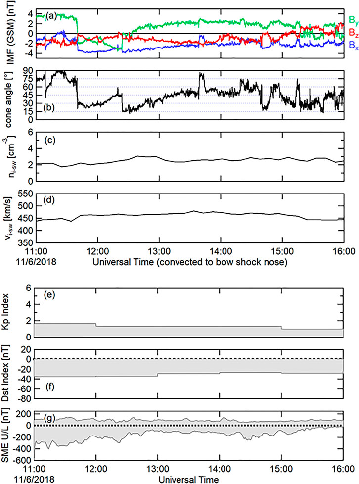
FIGURE 1. Observations of the solar wind by the ARTEMIS 1 spacecraft, convected in time by 11.2 min to the bow shock nose. (A) IMF components in GSM coordinates; (B) IMF cone angle; (C) Solar wind ion density; (D) Solar wind bulk speed; (E) Kp index; (F) Dst index; (G) SME U/L index (similar to the AE index).

There was no significant geomagnetic activity during this interval. The Kp index was <2 throughout the interval (Figure 1E), and the Dst index was > −40 nT during this time (Figure 1F). The SME U/L indices are SuperMAG derived indices (based on all available ground magnetometer stations at geomagnetic latitudes between +40° and +80°), provided in Figure 1G for context only, and are not officially authorized by the International Association of Geomagnetism and Aeronomy (IAGA). The SME U/L data products are similar to the traditional auroral electrojet indices (AE U/L) (Davis and Sugiura, 1966), as described in detail by Newell and Gjerloev (2011a,b). Based on these records, some modest auroral activity was present early during this interval of interest; but was not of great significance.

Locations of Sampling Spacecraft

Figure 2 shows the projected locations of multiple plasma and field sampling spacecraft during this time interval, in the GSM coordinate system. Figure 2A shows the projection into the XY (GSM equatorial) plane; Figure 2B shows the projection into the XZ (GSM noon-midnight meridian) plane. The magnetopause (Shue et al., 1997) and bow shock (Chao et al., 2002)–parameterized by the solar wind and including a small (4°) rotation to account for aberration of the solar wind - are provided for context. The Time History of Events and Macroscale Interactions during Substorms (THEMIS) A, D, and E spacecraft were all located in the dayside magnetosheath, north of the GSM equatorial plane at this time. These spacecraft did not observe any long period fluctuations in either the fields or plasma moments during this interval, and are not discussed further. The MMS constellation was at the dusk flank magnetopause, just past the terminator plane (i.e., X_GSM = 0), and was situated a couple R_E below the equatorial plane. The MMS spacecraft were on the inbound portion of the orbit, traveling normal to the magnetopause surface. Although it might at first appear that this is an unfortunate “angle of attack” of the magnetopause for studying KH, it actually provides for a relatively clean pass and sampling of the boundary, along with the plasma and magnetic fields of the magnetosheath proper and magnetosphere proper, which are also sampled relatively close in time to the observance of KH vortices. The Cluster set of spacecraft was also along the dusk flank; somewhat earthward of the magnetopause, and had crossed the GSM equatorial plane, moving from the southern magnetotail lobe to the northern lobe over the span of several hours. The Geotail spacecraft was also situated at the dusk flank magnetopause; a bit further downtail (X_GSM = ∼−12 R_E), but at higher southern latitude than any of the other spacecraft. The projection of a single magnetospheric magnetic field line is also shown, and will be discussed in further detail in Magnetic Field Mapping of Ionospheric “Bead”. Figure 2C uses the IMF cone angle and “clock angle” (convected to the bow shock, and then to the location of MMS) in conjunction with the YZ coordinates of the MMS spacecraft (a spatial “clock angle”) to construct a parameter “q”. This single parameter provides an assessment as to whether the magnetosheath region in the vicinity of MMS is downstream of the quasi-parallel bow shock (q > 0), or is downstream of the quasi-perpendicular bow shock (q < 0). Using this parameter, during the interval of ∼11:50—∼12:40 UT, the magnetosheath region near MMS was downstream of the quasi-parallel bow shock. Otherwise, the magnetosheath region near MMS is surmised to have been downstream of the quasi-perpendicular bow shock.

FIGURE 2

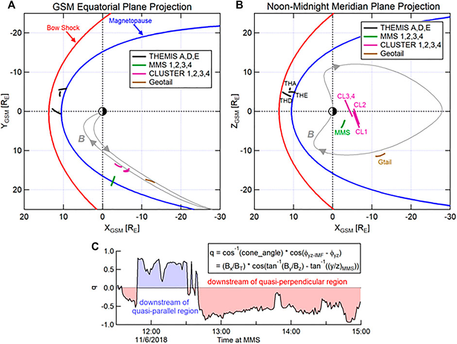
FIGURE 2. Spacecraft locations in GSM coordinates during the interval 2018-11-06, 11:30–15:00 UT. (A) Equatorial plane projection; (B) Meridian plane projection. The red trace demarks the parameterized bow shock shape and location; while the blue trace demarks the parameterized magnetopause shape and location. A magnetospheric magnetic field line (grey) is traced from the center location of the ionospheric bead in the northern ionosphere into the magnetotail and ending in the southern ionosphere. (C) Time series of parameter “q”. This parameter uses the ARTEMIS 1 IMF components (convected to the bow shock, plus an additional convection time of 7 mins) in conjunction with the MMS Y/Z location to determine whether the region local to MMS was downstream of the quasi-parallel bow shock (q > 0, in blue), or was downstream of the quasi-perpendicular bow shock (q < 0, in red).

MMS Observations

Figure 3 shows the plasma and magnetic field observations from the MMS1 spacecraft for a 3.5-h interval, as the spacecraft traveled from the magnetosheath into the magnetosphere. The four spacecraft of the MMS constellation were very close to one another (a few tens of km separation) at this time, and differences are negligible when viewed over larger time scales (hours). Therefore, the observations from MMS1 represent the observations from each of the spacecraft. The first panel of Figure 3 shows the GSE components of the magnetic field, and the magnetic field intensity is shown in the second panel. The third panel displays the overlaid time series of the ion (blue) and electron (red) number densities. The next three panels show the GSE components of the ion bulk velocity. The ion and electron temperatures parallel and perpendicular to the magnetic field are presented in the next two panels of Figure 3. The bottom panel shows the static pressure (P_Tot = n_ik_B(T_i-para + 2 T_i-perp)/3 + n_ek_B(T_e-para + 2 T_e-perp)/3 + B²/2μ₀).

FIGURE 3

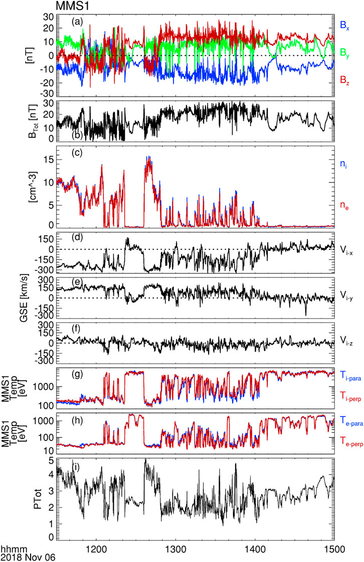
FIGURE 3. MMS observations of the magnetic field and plasma moments during the inbound traversal from the magnetosheath across the flank dusk magnetopause and into the magnetosphere. (A) Magnetic field components in GSE coordinates; (B) Magnetic field intensity; (C) Number densities of ions (blue) and electrons (red); (D) Ion bulk velocity component V_xGSE; (E) Ion bulk velocity components V_yGSE; (F) Ion bulk velocity components V_zGSE; (G) Perpendicular temperatures of ions (blue) and electrons (red); (H) Parallel temperatures of ions (blue) and electrons (red); and (I) Total static pressure (Sum of magnetic and thermal pressures).

Significant fluctuations were observed in all parameters as the MMS spacecraft passed from the magnetosheath into the magnetosphere, as displayed in Figure 3. As described earlier, the IMF orientation at the time suggests that the MMS spacecraft were downstream of the quasi-perpendicular bow shock. Therefore, it is not likely that these fluctuations were due to convected foreshock wave activity from the quasi-parallel bow shock. It was also noted that the solar wind bulk flow speed was considerably higher than average during this time. Higher solar wind speed has been shown to be statistically more conducive to initiate Kelvin-Helmholtz waves along the magnetopause, due to a larger velocity shear (e.g., Kavosi and Raeder, 2015). Figure 4 shows a 70-min expanded view focused on the fluctuations at the magnetopause, displaying the same set of panels as was shown in Figure 3. Variations in the ion number density are observed and exhibit the common and well-known feature of sharp increases followed by more gradual decreases associated with observations of rolled-up KH vortices at the magnetopause (cf., Chen et al., 1993; Hasegawa et al., 2004; Hasegawa et al., 2006; Hasegawa et al., 2009).

FIGURE 4

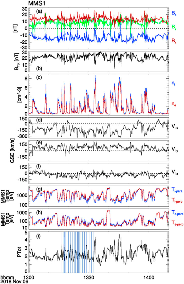
FIGURE 4. Expanded view of sub-interval from Figure 3. This sub-interval lies between the magnetosheath proper and magnetosphere proper, and shows several brief crossings of the magnetopause boundary. Panel format is the same as that of Figure 3. Blue vertical lines in the bottom panel demark peaks of the static pressure.

An often-used test for the onset of the KHI for an ideal, incompressible plasma across a thin velocity shear layer satisfies the following inequality (Chandrasekhar, 1961; Henry et al., 2017):

${\left[\mathit{k}\cdot \left({\mathit{v}}_{\mathbf{1}}-{\mathit{v}}_{\mathbf{2}}\right)\right]}^{\mathbf{2}}\ge \frac{{\mathit{n}}_1+{\mathit{n}}_2}{4\mathit{\pi }{\mathit{m}}_0{\mathit{n}}_1{\mathit{n}}_2}\left[{\left(\mathit{k}\cdot {\mathit{B}}_{\mathbf{1}}\right)}^{\mathbf{2}}+{\left(\mathit{k}\cdot {\mathit{B}}_{\mathbf{2}}\right)}^{\mathbf{2}}\right](1)$

and is tested across the flank magnetopause. The subscript “1” refers to the magnetosheath proper, and subscript “2” refers to the magnetosphere proper. The methodology for determining these regions is based on the description of Henry et al., 2017. The average of the highest and lowest quartiles of the ratio n_i/T_i are used to determine “the magnetopause” value of n_i/T_i. Larger values are designated to “the magnetosheath”; lower values are designated to “the magnetosphere”. The top one-third of the ranked n_i/T_i ratio of “the magnetosheath” population is used to determine the mean vector and scalar components for the magnetosheath proper. Similarly, the lowest one-third of “the magnetosphere” population is used to determine the mean vector and scalar components for the magnetosphere proper. The mean vector (GSE) components and ion number density values are thus as follows: B₁ = {−7.738, 6.977, −2.593} nT; B₂ = {−5.925, 3.965, 10.009} nT; V₁ = {−261.563, 145.446, 29.466} km/s; V₂ = {13.953, 0.189, −0.215} km/s; n₁ = 10.336 cm⁻³; n₂ = 0.290 cm⁻³. Using these mean plasma moment and magnetic field vector values for the magnetosheath proper and for the magnetosphere proper, the unit k-vector corresponding to maximum wave growth is: {−0.736, −0.668, −0.114}. With this unit k-vector, the ratio of the left hand side to the right hand side of the inequality of Eq. 1 is 2.95; easily satisfying this test for the presence of a Kelvin-Helmholtz instability. As shown in Figure 1, the IMF was steady and slightly southward during most of this time interval. Although the Kelvin-Helmholtz instability commonly occurs along Earth’s low-latitude magnetopause flanks during sustained intervals of northward IMF (e.g., Kavosi and Raeder, 2015), it is occasionally observed during intervals of southward IMF. About 10% of all KH intervals occurred during southward IMF as reported in the statistical study by Kavosi and Raeder, (2015), while a larger percentage of KH intervals were reported to occur during southward IMF by Henry et al. (2017). Individual cases of flank magnetopause Kelvin-Helmholtz occurring during southward IMF were investigated by Hwang et al. (2011); Nakamura et al. (2020); Kronberg et al. (2021).

A second diagnostic to test for the presence of Kelvin-Helmholtz observed by the MMS spacecraft at the magnetopause is to plot the bulk velocity as a function of the ion density. The presence of low ion density at high tailward velocity is suggestive of the mixing of plasmas and the occurrence of well-developed rolled-up vortices, as described by both models and observations (Hasegawa et al., 2004, 2006; Takagi et al., 2006; Taylor et al., 2012). The maximum variance of the magnetosheath electric field (-vxB) is estimated via the MVA-E method (Sonnerup and Scheible, 1998), and provides the bulk velocity tangential to the magnetopause, which is displayed in Figure 5. The data points in the region below the red dashed curve provide evidence for the presence of rolled-up vortices, and is consistent with the results of the first diagnostic test. It is therefore concluded from the results of these diagnostic tests that KH waves were observed along the dusk flank magnetopause by MMS.

FIGURE 5

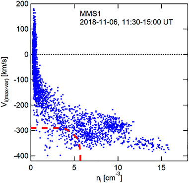
FIGURE 5. MMS ion bulk velocity along maximum variance direction during this interval, as a function of the ion number density. Positive velocities are in the sunward direction. Low density, larger anti-sunward speeds (below the red dashed curve) are indicative of Kelvin-Helmholtz activity, with plasma mixing within well-developed vortices.

Cluster Observations

As described above (and shown in Figure 2), the four Cluster spacecraft were relatively close to the MMS constellation during this interval; but were located slightly further within the magnetotail. The four Cluster spacecraft were traveling northward from south of the GSM equator along their respective orbits during this interval, and all four observed clear oscillations in the magnetic field components and intensity. Although it is not proven here that the KH waves along the dusk flank magnetopause drove the magnetic field oscillations observed at Cluster, past observational studies have established an observations-based connection between KH waves along the magnetopause and the excitation of ULF waves observed within the magnetosphere and on the ground (e.g., Mann et al., 2002; Rae et al., 2005). The Lyon-Fedder-Mobarry (LFM) global, three-dimensional magnetohydrodynamic (MHD) single-fluid simulations has also been shown that ULF pulsations can be generated near the flank magnetopause in response to the magnetopause KH instability (Claudepierre et al., 2008). A recent study by Kim et al. (2021) also shows how KH waves may couple to Alfvén waves in the magnetosphere. In contrast to the MMS observations of fluctuations at the magnetopause, the magnetic field transverse and compressional fluctuations observed at Cluster are of a more sinusoidal nature.

Wave periods are determined during the interval of greatest observed wave activity in the maximum variance direction of the Cluster magnetic field; i.e., from estimates of peak-to-peak times during 12:30 to 15:41 UT. The Cluster 3 and 4 spacecraft were very close to one another during this time interval, with a separation distance of ∼13.5 km at 10:30 UT, decreasing to ∼11.0 km at 16:00 UT. As would be expected from spacecraft in such proximity, the observed magnetic field variations are nearly identical (Figure 6): with a correlation coefficient of r > +0.999. The average and standard deviation of the wave period was 7.5 ± 2.9 min (frequencies of 1.6—5.7 mHz). In comparison (Figure 7), the Cluster 1 and 2 pair of spacecraft were further separated from one another than the Cluster 3,4 pair: from ∼6,000 km at 10:30 UT, decreasing to ∼5,300 km at 16:00 UT. The average and standard deviation of the wave period was 7.6 ± 3.2 min (frequencies of 1.5—3.8 mHz), with a high correlation coefficient (r = +0.92); though not quite as high as the correlation between Cluster 3 and 4. The Cluster 1 and 2 pair of spacecraft were significantly distant from the Cluster 3 and 4 spacecraft (∼3.1–4.5 R_E distant).

FIGURE 6

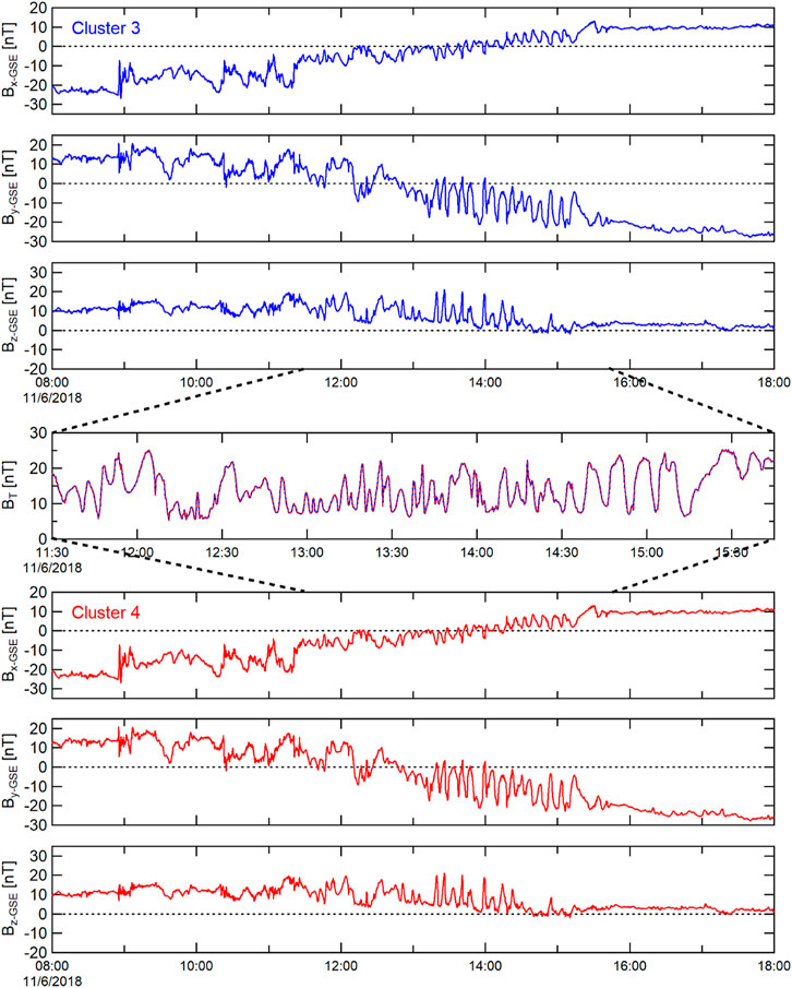
FIGURE 6. Magnetic field observations from Cluster 3 and Cluster 4, in GSE coordinates. These spacecraft were initially in the southern lobe (strong and rather steady negative B_x), and ended in the northern magnetotail lobe (strong and rather steady positive B_x). During the time spent near the magnetopause and flank neutral sheet, coherent transverse and compressional waves were observed in the magnetic field. Magnetic field intensity (and compressional waves) from the two spacecraft are overlaid in the fourth (middle) panel, and are essentially identical in amplitude, frequency, and phase. Highest frequency waves are closest to the neutral sheet (B_x near zero).

FIGURE 7

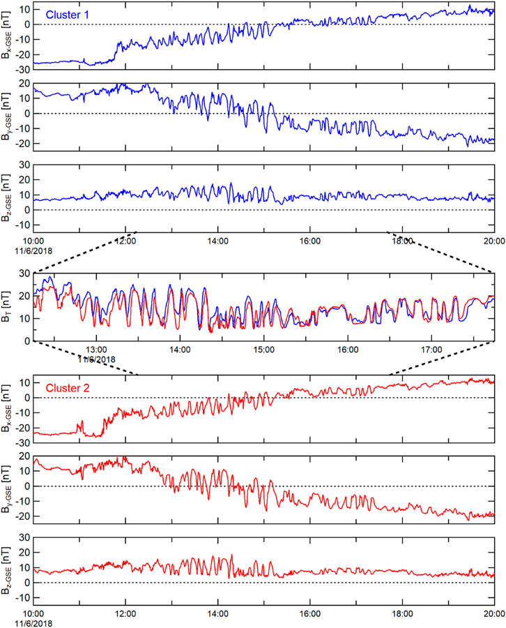
FIGURE 7. Magnetic field observations from Cluster 1 and Cluster 2, in GSE coordinates. Panel format is the same as that of Figure 6.

The frequency range of the Cluster magnetic field fluctuations overlaps substantially with the ULF frequency range found in the LFM simulations by Claudepierre et al. (2008) within the magnetosphere (0.5—3 mHz). The magnetic field oscillations were also of similar frequency to long-period ULF waves in the plasma sheet as described by Tian et al. (2012) (1.7—2.0 and 3.0—3.2 mHz). The location of the spacecraft is consistent with being near the magnetopause edge of the magnetotail plasma sheet. Cluster Ion Spectrometry (CIS) plasma moment data were available during this time. However, the observed plasma moments showed no significant variations; in contrast to the magnetic field. The observed proton density remained relatively constant; between ∼0.1 and ∼0.3 cm⁻³ throughout this entire interval (not shown).

Geotail Observations

The Geotail magnetic field, electron and proton energy flux spectrograms are shown in Figure 8, plotted over a 6-h interval (12:00—18:00 UT). A >1-h data gap occurred between ∼15:30—16:25 UT. The components and intensity of the magnetic field were fairly steady during the first few hours of this interval, and are consistent with the expectations of the Geotail spacecraft being located within the magnetotail, south of the neutral sheet. Small oscillations of the magnetic field (a few nT) were observed after ∼14:25 UT. The magnetic field fluctuations did not exhibit any significant linear or circular polarization. The diminished magnetic field fluctuations relative to those observed at Cluster is consistent with the LFM numerical simulations of Claudepierre et al. (2008); which suggests that the ULF integrated wave power as driven by KH decreases markedly with distance downtail, and with distance away from the GSM equator.

FIGURE 8

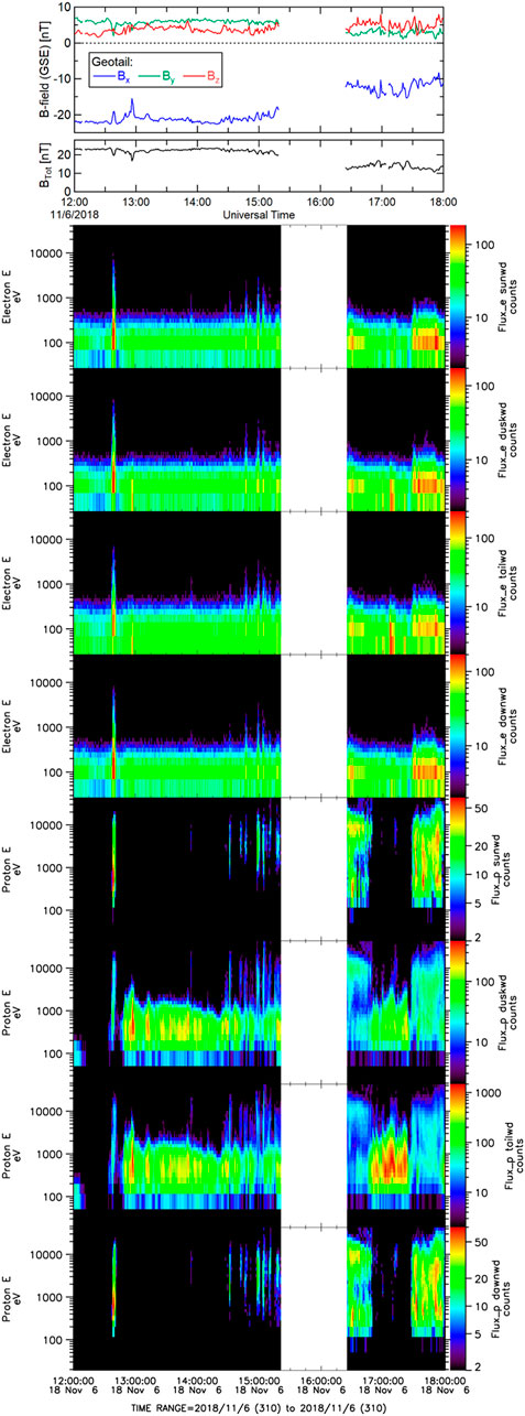
FIGURE 8. Geotail observations of the magnetic field, electron energy flux spectrograms, and proton energy flux spectrograms observed in four directions. Color scale of flux min/max values are auto-scaled within each panel.

The electron and proton energy flux spectrograms from the Geotail LEP instrument during this interval are also shown in Figure 8, segregated into four distinct sectors designating plasma flow directions: Sunward, duskward, tailward, and dawnward. For the electron energy flux spectrograms, equal flux was observed in all directions, with an energy of ∼100 eV. For the proton energy flux spectrograms, significant flux was only observed moving towards dusk and downtail, with an energy of several hundred eV. These observations are consistent with the spacecraft sampling the plasma mantle (cf., Rosenbauer et al., 1975; Haaland et al., 2008).

Starting just prior to 14:30 UT, enhancements in the electron flux appear in all directions; while the peak energy remains at ∼100 eV. Coincident with the electron flux enhancements, proton flux enhancements are also observed. The proton flux enhancements are also seen in all directions, and are at higher energy (peaked at a few to several keV). An expanded (90-min) view of these flux enhancements (along with the magnetic field) is shown in Figure 9. The enhancements are likely due to brief excursions into the plasma sheet boundary layer. The enhancements are somewhat periodic, with eight enhancements occurring within the span of about hour (period of ∼7 min; or frequency of ∼2.4 mHz). This frequency is within the frequency band observed by the Cluster magnetometers, and suggests that the flux enhancements observed at Geotail are related to the ULF wave activity observed by Cluster.

FIGURE 9

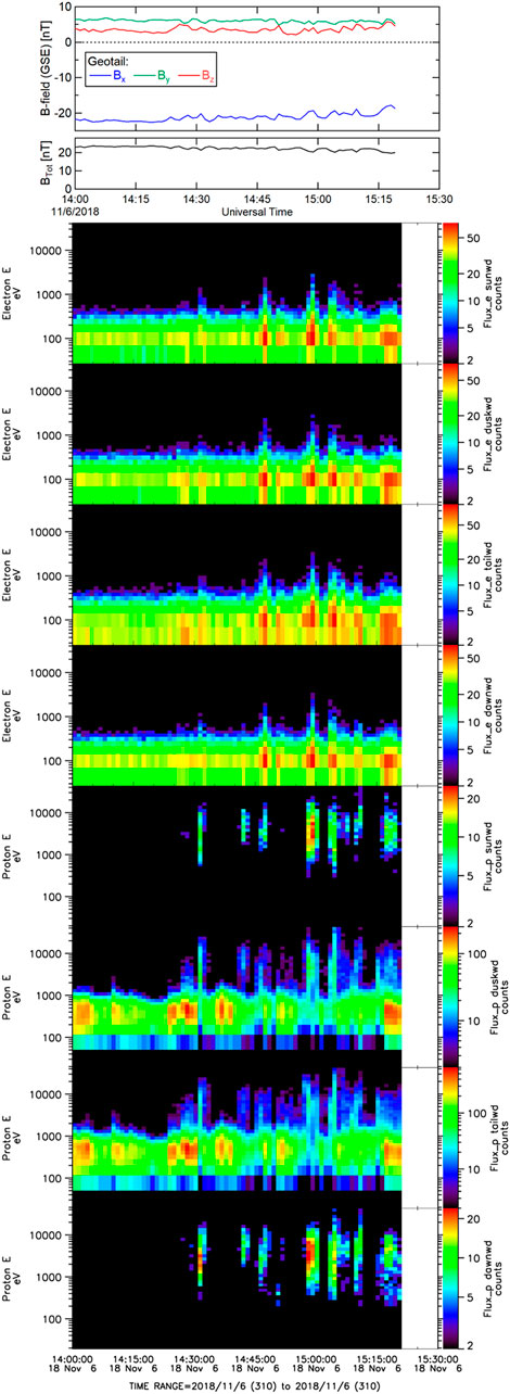
FIGURE 9. Expanded view of the Geotail magnetic field and electron and proton energy flux spectrograms. Layout is the same as Figure 8.

DMSP Observations of a Dayside Ionosphere “Bead”

DMSP satellites imaged significant portions of the auroral oval several times during this KH event. Figure 10A presents an example of an auroral oval in the northern hemisphere imaged DMSP SSUSI at ∼11:40–12:00 UT. This time is near the start of the larger time interval when fluctuations were observed by the various spacecraft, as described above. The image reveals several bead structures can be seen more clearly in the zoomed in image presented in Figure 10B. Although the DMSP satellite re-visited and images the northern auroral region every ∼101 min, due to the precession of the magnetic dipole, subsequent passes did not provide image coverage of the same auroral region near local noon. Although this particular DMSP SSUSI observation occurred just prior to the MMS spacecraft encountering the flank magnetopause, this interval does coincide with the Cluster 3 and 4 observations of ULF pulsations just inside the flank magnetopause (starting ∼11:30 UT). As described above, these pulsations are believed to occur in response to KH activity (Claudepierre et al., 2008).

FIGURE 10

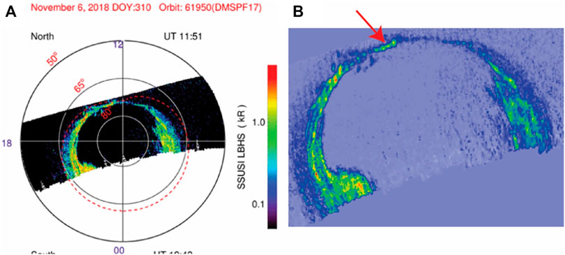
FIGURE 10. (A) DMSP SSUSI LBHS image of the auroral bead on 2018-11-06 11:40–12:00 UT. (B) A zoomed in version of auroral emissions shown in panel (A). The red arrow shows the bead that is analyzed in DMSP Observations of a Dayside Ionosphere “Bead”.

Recently, Johnson et al. (2021) developed a theory for mesoscale field-aligned currents generated by the KH vortices at the magnetopause boundary layer. The theory predicts that the mapping of the KH vortex to the ionosphere is optimal when Λ/L = 2.8, where Λ = width of the vortex field-aligned current, L = the auroral electrostatic scale length = $\sqrt{\raisebox{1ex}{${\text{Σ}}_p$}\!\left/ \!\raisebox{-1ex}{$\kappa $}\right.}$, Σ_p = Pedersen conductivity, and κ = Knight κ (Knight, 1973). The assumption of the linear approximation to the Knight current-voltage relation is used: j = κΦ, and κ = e²n_e/(2π m_eT_e)^1/2; where j and Φ represent the field-aligned current density and field-aligned potential, respectively. Moreover, they demonstrated that the theory can predict the KH vortex size at the magnetopause boundary layer from DMSP and THEMIS observations in one event.

A theory–observation comparison using DMSP and MMS observations is conducted here, as was done in Johnson et al. (2021). For the analysis, the focus is on a bead pointed to by the red arrow in Figure 10B. The bead is centered at (Mlat, MLT) = (76.5°, 14.1) and Λ = 93 km. Using the solar zenith angle at this location (χ ∼ 6°) and F10.7 solar flux density = 68 W m⁻² Hz⁻¹, the Pedersen conductivity due to the ionizing solar extreme ultraviolet (EUV) radiation is Σ_p,s = 7 S (Robinson and Vondrak, 1984). Inside the bead, the mean energy is estimated to be 8 keV and the mean energy flux to be 18 erg s⁻¹ cm⁻² based on N₂ LBHS (140–150 nm) and LBHL (165–180 nm) radiances (Zhang and Paxton, 2008 and references therein) observed by DMSP SSUSI (Paxton et al., 1993). Using these values, the Pedersen conductivity due to electron precipitation is estimated as Σ_p,e = 17 S (Robinson et al., 1987). The total ${\text{Σ}}_p=\sqrt{{\text{Σ}}_{p,e}^2+ {\text{Σ}}_{p,s}^2}$ ∼ 18 S (Wallis and Budzinski, 1981).

MMS provides observations of T_e = 39.7 eV, n_e = 2.9 cm⁻³, |B|_MMS = 20.5 nT near the center of the KH vortex at the boundary layer. Using the Knight κ calculated from MMS T_e and n_e and Σ_p calculated from DMSP observations, values of L = 39 km and Λ/L = 2.4 are obtained, which is close to the Johnson et al. (2021) theoretical optimal value for mapping the vortex to the ionosphere: Λ/L = 2.8.

The predicted KH vortex spatial scale is calculated from Λ, L, B_i, and B_m where B_m = |B|_MMS, and B_i = |B|_DMSP = 39,759 nT. Johnson et al. (2021) derived an expression for Δ_i = 2 α L = 49 km, where Δ_i = the vortex radius mapped to the ionosphere and α = a mapping parameter obtained from Λ/L (|x|/L = 2 Λ/L) as described in Figure 3 in Johnson et al. (2021). The radius of the KH vortex at the boundary layer Δ_m = b Δ_i = 2,162 km, where b = (B_i/B_m)^1/2. The diameter of the KH vortex = 4325 km (∼0.68 RE), where R_E = radius of the Earth = 6,372 km. This size is compared with that estimated from the MMS observation. The estimate from Figure 3 is that the KH wavelength = 1.5 R_E, using the number of identified static pressure peaks between 13:17 and 13:32 UT to estimate the wave period, and using the bulk speed at the center of the vortex (at 13:25:18 UT, identified from the local minima observed in the |V_i-N|, |V_i-M|, and |B_N| components, where the GSE–> LMN coordinate transformation was determined from the MVA-E method mentioned earlier, and used in the diagnostic test of Figure 5). Otto and Fairfield (2000) found that KH vortex size is about one-half the wavelength. Using this ratio of KH wavelength to diameter, the estimate of the observed KH diameter = 0.75 R_E, which is close to the predicted value of 0.68 R_E. Using the peak value ε_max from Figure 7 of Johnson et al. (2021), the predicted maximum current density using observed KH vortex parameters is j_||,_max = 45 μA/m².

In the above calculation, Σ_p,e was estimated from the precipitating electron energy flux (J_e) and mean energy (E_e) inside the bead from DMSP SSUSI LBHS and LBHL emissions using the method described in Zhang and Paxton (2008). The estimated J_e and E_e have relatively large statistical errors due to limited counts in the LBHS and LBHL channels. The estimated values of J_e = 18 erg s⁻¹ cm⁻² and E_e = 7 keV are probably too high, which leads to a rather high estimated value of Σ_p,e = 17 S (Robinson et al., 1987; Johnson and Wing, 2015; Wing and Johnson, 2015). If a value of Σ_p,e = 5 S is used (resulting in total Σ_p = 8.6 S), then a value of Λ/L = 3.5 would have been obtained, with a predicted KH vortex diameter = 0.72 R_E. It is interesting to note that the predicted KH diameter of 0.72 R_E would be closer to the observed value of 0.75 R_E, although the value of Λ/L = 3.5 would represent a larger deviation from the theoretical optimal value of 2.8. It is also interesting to note that in this particular event, changing Σ_p from 17 to 8.6 S would result in only a small change of the predicted KH diameter; from 0.68 R_E to 0.72 R_E. Using the peak ε_max from Johnson et al. (2021), the predicted maximum parallel current density is then significantly reduced (j_||,_max = 21 μA/m²).

Magnetic Field Mapping of Ionospheric “Bead”

The Tsyganenko 1996 magnetospheric magnetic field model (Tsyganenko, 1995) has been used to trace the magnetic field from the center location of the ionospheric bead out into the magnetosphere. The traced magnetic field line extends from the post-noon high-latitude ionosphere to the deep magnetotail, to X_GSM = ∼−28 R_E downtail (shown in gray in Figure 2). This field line trace is also close to the dusk flank magnetopause, in the same general region as the sampling spacecraft previously discussed. Continuing the trace to the southern hemisphere, the magnetic field line associated with the ionospheric bead passed very close to the location of Geotail.

Conclusions and Summary

During an extended interval on 2018 November 06, Kelvin-Helmholtz wave activity was observed by multiple instruments on board the MMS spacecraft at the dusk flank magnetopause. The solar wind during this time was slightly faster than the nominal solar wind; but was steady with a slightly southward B_z-GSM component. Additional spacecraft (Cluster at low latitudes; Geotail at mid-latitude) within the dusk flank magnetotail near the magnetopause also observed wave activity in the magnetic field and plasma fluxes. However, this wave activity was more coherent than that observed at MMS, consistent with ULF waves driven by the Kelvin-Helmholtz wave activity at the magnetopause. The observed magnetic field ULF wave activity is consistent in location and in frequency range with the global MHD simulation results described by Claudepierre et al. (2008). Fluctuations in ion and electron fluxes were also observed further downtail within the plasma mantle close to the duskside magnetopause by Geotail; with a periodicity similar to that of the ULF magnetic field waves observed by the Cluster spacecraft.

DMSP SSUSI LBHS observations of an ionospheric bead structure in the post-noon high-latitude region along with observed properties of the KH vortices along the flank magnetopause have been used to successfully test a theory of mesoscale field-aligned currents generated by KH vortices. This theory (Johnson et al., 2021) predicts that the optimal mapping of the KH vortex to the ionosphere occurs when Λ/L (= 2.8). Observations have provided a value of close to the optimal value. This theoretical treatment has also been used to show that ionospheric observations along with a mapping relation can provide an estimate of the KH vortex size, which is very similar to the size determined from the in situ observations of KH vortices (d = ∼0.7 R_E).

To summarize, an extended, seredipitous interval of multi-spacecraft observations along the dusk flank magnetopause and at low Earth orbit has been investigated. KH vortices observed at the magnetopause boundary layer are associated with ULF waves observed just inside of the flank magnetopause, along with a successful testing of parameters associating an observed pre-noon high-latitude ionospheric “bead” with the KH vortices along the flank magnetopause.

Data Availability Statement

Publicly available datasets were analyzed in this study. This data can be found here: http://cdaweb.gsfc.nasa.gov/istp_public/, https://lasp.colorado.edu/mms/sdc/public/about/, https://ssusi.jhuapl.edu/gal_edr-aur_cs, https://ccmc.gsfc.nasa.gov/modelweb/magnetos/tsygan.html.

Author Contributions

SP plotted and analyzed the solar wind, geomagnetic, and magnetopause flank spacecraft data sets. He also traced the magnetic field line from the ionosphere into the magnetotail. SW identified the ionospheric bead and provided estimates of the conductivity. SW and JJ provided estimates of the energy flux, and scale sizes of the bead and vortex, and comparisons with a theory of mesoscale field-aligned currents generated by KH vortices and optimal mapping criterion. YZ created the DMSP SSUSI map of auroral emissions.

Funding

Research at Lockheed Martin was performed on Contracts 499935Q, 80NSSC18K1379, and 80NSSC17K0643 (sub-contract 18-027). SW acknowledges the support of NASA Grants 80NSSC20K0704, 80NSSC19K0843, 80NSSC19K0822, 80NSSC20K0188, 80NSSC20K1279, and 80NSSC21K1678. JJ acknowledges support from NASA grants NNX15AJ01G, NNX16AQ87G, 80NSSC19K0843, NNX17AI50G, and 80NSSC20K0704. YZ acknowledges the support of USAF Contract N00024-13-D-6400.

Conflict of Interest

The authors declare that the research was conducted in the absence of any commercial or financial relationships that could be construed as a potential conflict of interest.

Publisher’s Note

All claims expressed in this article are solely those of the authors and do not necessarily represent those of their affiliated organizations, or those of the publisher, the editors, and the reviewers. Any product that may be evaluated in this article, or claim that may be made by its manufacturer, is not guaranteed or endorsed by the publisher.

Acknowledgments

The women and men that worked and continue to work on these missions share in their successes.

References

Auster, H. U., Glassmeier, K. H., Magnes, W., Aydogar, O., Baumjohann, W., Constantinescu, D., et al. (2008). The THEMIS Fluxgate Magnetometer. Space Sci. Rev. 141, 235–264. doi:10.1007/s11214-008-9365-9

CrossRef Full Text | Google Scholar

Balogh, A., Dunlop, M. W., Dunlop, M. W., Cowley, S. W. H., Southwood, D. J., Thomlinson, J. G., et al. (1997). The Cluster Magnetic Field Investigation. Space Sci. Rev. 79, 65–91. doi:10.1023/A:100497090774810.1007/978-94-011-5666-0_3

CrossRef Full Text | Google Scholar

Chandrasekhar, S. (1961). Hydrodynamic and Hydromagnetic Stability. New York: Oxford University Press.

Google Scholar

Chao, J. K., Wu, D. J., Lin, C.-H., Yang, Y.-H., Wang, X. Y., Kessel, M., et al. (2002). “Models for the Size and Shape of the Earth's Magnetopause and bow Shock,” in Space Weather Study Using Multipoint Techniques, COSPAR Colloq. Ser. Editor L.-H. Lyu (Oxford: Pergamon), Vol. 12, 127–135. doi:10.1016/s0964-2749(02)80212-8

CrossRef Full Text | Google Scholar

Chen, S.-H., Kivelson, M. G., Gosling, J. T., Walker, R. J., and Lazarus, A. J. (1993). Anomalous Aspects of Magnetosheath Flow and of the Shape and Oscillations of the Magnetopause during an Interval of Strongly Northward Interplanetary Magnetic Field. J. Geophys. Res. 98, 5727–5742. doi:10.1029/92JA02263

CrossRef Full Text | Google Scholar

Chen, S.-H., and Kivelson, M. G. (1993). On Nonsinusoidal Waves at the Earth‧s Magnetopause. Geophys. Res. Lett. 20, 2699–2702. doi:10.1029/93GL02622

CrossRef Full Text | Google Scholar

Claudepierre, S. G., Elkington, S. R., and Wiltberger, M. (2008). Solar Wind Driving of Magnetospheric ULF Waves: Pulsations Driven by Velocity Shear at the Magnetopause. J. Geophys. Res. 113, a–n. doi:10.1029/2007JA012890

CrossRef Full Text | Google Scholar

Couzens, D., Parks, G. K., Anderson, K. A., Lin, R. P., and Reme, H. (1985). ISEE Particle Observations of Surface Waves at the Magnetopause Boundary Layer. J. Geophys. Res. 90, 6343–6353. doi:10.1029/JA090iA07p06343

CrossRef Full Text | Google Scholar

Davis, T. N., and Sugiura, M. (1966). Auroral Electrojet Activity indexAEand its Universal Time Variations. J. Geophys. Res. 71, 785–801. doi:10.1029/JZ071i003p00785

CrossRef Full Text | Google Scholar

Dmitriev, A. V., and Suvorova, A. V. (2015). Large‐scale Jets in the Magnetosheath and Plasma Penetration across the Magnetopause: THEMIS Observations. J. Geophys. Res. Space Phys. 120 (6), 4423–4437. doi:10.1002/2014JA020953

CrossRef Full Text | Google Scholar

Dmitriev, A. V., and Suvorova, A. V. (2012). Traveling Magnetopause Distortion Related to a Large-Scale Magnetosheath Plasma Jet: THEMIS and Ground-Based Observations. J. Geophys. Res. 117, a–n. doi:10.1029/2011JA016861

CrossRef Full Text | Google Scholar

Fairfield, D. H., Otto, A., Mukai, T., Kokubun, S., Lepping, R. P., Steinberg, J. T., et al. (2000). Geotail Observations of the Kelvin-Helmholtz Instability at the Equatorial Magnetotail Boundary for Parallel Northward fields. J. Geophys. Res. 105 (A9), 21159–21173. doi:10.1029/1999JA000316

CrossRef Full Text | Google Scholar

Haaland, S., Paschmann, G., Förster, M., Quinn, J., Torbert, R., Vaith, H., et al. (2008). Plasma Convection in the Magnetotail Lobes: Statistical Results from Cluster EDI Measurements. Ann. Geophys. 26, 2371–2382. doi:10.5194/angeo-26-2371-2008

CrossRef Full Text | Google Scholar

Hasegawa, H., Fujimoto, M., Phan, T.-D., Rème, H., Balogh, A., Dunlop, M. W., et al. (2004). Transport of Solar Wind into Earth's Magnetosphere through Rolled-Up Kelvin-Helmholtz Vortices. Nature 430, 755–758. doi:10.1038/nature02799

PubMed Abstract | CrossRef Full Text | Google Scholar

Hasegawa, H., Fujimoto, M., Takagi, K., Saito, Y., Mukai, T., and Rème, H. (2006). Single-spacecraft Detection of Rolled-Up Kelvin-Helmholtz Vortices at the Flank Magnetopause. J. Geophys. Res. 111, A09203. doi:10.1029/2006JA011728

CrossRef Full Text | Google Scholar

Hasegawa, H., Retinò, A., Vaivads, A., Khotyaintsev, Y., André, M., Nakamura, T. K. M., et al. (2009). Kelvin-Helmholtz Waves at the Earth's Magnetopause: Multiscale Development and Associated Reconnection. J. Geophys. Res. 114, a–n. doi:10.1029/2009JA014042

CrossRef Full Text | Google Scholar

Henry, Z. W., Nykyri, K., Moore, T. W., Dimmock, A. P., and Ma, X. (2017). On the Dawn-Dusk Asymmetry of the Kelvin-Helmholtz Instability between 2007 and 2013. J. Geophys. Res. Space Phys. 122, 888–911. doi:10.1002/2017JA024548

CrossRef Full Text | Google Scholar

Holzer, R. E., McLeod, M. G., and Smith, E. J. (1966). Preliminary Results from the Ogo 1 Search Coil Magnetometer: Boundary Positions and Magnetic Noise Spectra. J. Geophys. Res. 71, 1481–1486. doi:10.1029/JZ071i005p01481

CrossRef Full Text | Google Scholar

Hones, E. W., BirnAsbridge, J. J. R., BamePaschmannSckopke, S. J. G. N., Asbridge, J. R., Paschmann, G., Sckopke, N., et al. (1981). Further Determination of the Characteristics of Magnetospheric Plasma Vortices with ISEE 1 and 2. J. Geophys. Res. 86, 814–820. doi:10.1029/ja086ia02p00814

CrossRef Full Text | Google Scholar

Howe, H. C., and Siscoe, G. L. (1972). Magnetopause Motions at Lunar Distance Determined from the Explorer 35 Plasma experiment. J. Geophys. Res. 77, 6071–6086. doi:10.1029/JA077i031p06071

CrossRef Full Text | Google Scholar

Hwang, K.-J., Kuznetsova, M. M., Sahraoui, F., Goldstein, M. L., Lee, E., and Parks, G. K. (2011). Kelvin-Helmholtz Waves under Southward Interplanetary Magnetic Field. J. Geophys. Res. 116, a–n. doi:10.1029/2011JA016596

CrossRef Full Text | Google Scholar

Hwang, K.-J. (2015). Magnetopause Waves Controlling the Dynamics of Earth's Magnetosphere. J. Astron. Space Sci. 32 (1), 1–11. doi:10.5140/JASS.2015.32.1.1

CrossRef Full Text | Google Scholar

Johnson, J. R., Wing, S., Delamere, P., Petrinec, S., and Kavosi, S. (2021). Field‐Aligned Currents in Auroral Vortices. J. Geophys. Res. Space Phys. 126, e2020JA028583. doi:10.1029/2020JA028583

CrossRef Full Text | Google Scholar

Johnson, J. R., and Wing, S. (2015). The Dependence of the Strength and Thickness of Field‐aligned Currents on Solar Wind and Ionospheric Parameters. J. Geophys. Res. Space Phys. 120, 3987–4008. doi:10.1002/2014JA020312

CrossRef Full Text | Google Scholar

Kaufmann, R. L., and Konradi, A. (1969). Explorer 12 Magnetopause Observations: Large-Scale Nonuniform Motion. J. Geophys. Res. 74, 3609–3627. doi:10.1029/JA074i014p03609

CrossRef Full Text | Google Scholar

Kavosi, S., and Raeder, J. (2015). Ubiquity of Kelvin-Helmholtz Waves at Earth's Magnetopause. Nat. Commun. 6, 7019. doi:10.1038/ncomms8019

PubMed Abstract | CrossRef Full Text | Google Scholar

Kim, E.-H., Johnson, J. R., and Nykyri, K. (2021). Coupling between Alfven Wave and Kelvin-Helmholtz Waves in the Low Latitude Boundary Layer. Front. Phys. doi:10.3389/fphy.2021.785413

CrossRef Full Text | Google Scholar

Kivelson, M. G., and Chen, S.-H. (1995). “The Magnetopause: Surface Waves and Instabilities and Their Possible Dynamic Consequences,” in Physics of the Magnetopause, Geophys. Monogr. Ser. Editors P. Song, B. U. Ö. Sonnerup, and M. F. Thomsen (Washington D.C.: AGU), Vol. 90, 257–268.

Google Scholar

Kivelson, M. G., and Zu-Yin, P. (1984). The Kelvin-Helmholtz Instability on the Magnetopause. Planet. Space Sci. 32, 1335–1341. doi:10.1016/0032-0633(84)90077-1

CrossRef Full Text | Google Scholar

Knight, S. (1973). Parallel Electric fields. Planet. Space Sci. 21 (5), 741–750. doi:10.1016/0032-0633(73)90093-7

CrossRef Full Text | Google Scholar

Kokubun, S., Yamamoto, T., Acuña, M. H., Hayashi, K., Shiokawa, K., and Kawano, H. (1994). The GEOTAIL Magnetic Field experiment. J. Geomagn. Geoelec 46, 7–21. doi:10.5636/jgg.46.7

CrossRef Full Text | Google Scholar

Kronberg, E. A., Gorman, J., Nykyri, K., Smirnov, A. G., Gjerloev, J. W., Grigorenko, E. E., et al. (2021). Kelvin-Helmholtz Instability Associated with Reconnection and Ultra Low Frequency Waves at the Ground: A Case Study. Front. Phys. 9. doi:10.3389/fphy.2021.738988

CrossRef Full Text | Google Scholar

Lee, L. C., Albano, R. K., and Kan, J. R. (1981). Kelvin-Helmholtz Instability in the Magnetopause-Boundary Layer Region. J. Geophys. Res. 86, 54–58. doi:10.1029/JA086iA01p00054

CrossRef Full Text | Google Scholar

Li, H., Jiang, W., Wang, C., Verscharen, D., Zeng, C., Russell, C. T., et al. (2020). Evolution of the Earth's Magnetosheath Turbulence: A Statistical Study Based on MMS Observations. ApJ 898 (2), L43. doi:10.3847/2041-8213/aba531

CrossRef Full Text | Google Scholar

Lui, A. T. Y., Venkatesan, D., and Murphree, J. S. (1989). Auroral Bright Spots on the Dayside Oval. J. Geophys. Res. 94, 5515–5522. doi:10.1029/JA094iA05p05515

CrossRef Full Text | Google Scholar

Mann, I. R., Voronkov, I., Dunlop, M., Donovan, E., Yeoman, T. K., Milling, D. K., et al. (2002). Coordinated Ground-Based and Cluster Observations of Large Amplitude Global Magnetospheric Oscillations during a Fast Solar Wind Speed Interval. Ann. Geophys. 20, 405–426. doi:10.5194/angeo-20-405-2002

CrossRef Full Text | Google Scholar

McFadden, J. P., Carlson, C. W., Larson, D., Bonnell, J., Mozer, F., Angelopoulos, V., et al. (2008b). THEMIS ESA First Science Results and Performance Issues. Space Sci. Rev. 141, 477–508. doi:10.1007/s11214-008-9433-1

CrossRef Full Text | Google Scholar

McFadden, J. P., Carlson, C. W., Larson, D., Ludlam, M., Abiad, R., Elliott, B., et al. (2008a). The THEMIS ESA Plasma Instrument and In-Flight Calibration. Space Sci. Rev. 141, 277–302. doi:10.1007/s11214-008-9440-2

CrossRef Full Text | Google Scholar

Miura, A. (1995). Dependence of the Magnetopause Kelvin-Helmholtz Instability on the Orientation of the Magnetosheath Magnetic Field. Geophys. Res. Lett. 22, 2993–2996. doi:10.1029/95GL02793

CrossRef Full Text | Google Scholar

Mukai, T., Machida, S., Saito, Y., Hirahara, M., Terasawa, T., Kaya, N., et al. (1994). The Low Energy Particle (LEP) Experlment Onboard the GEOTAIL Satellite. J. Geomagn. Geoelec 46, 669–692. doi:10.5636/jgg.46.669

CrossRef Full Text | Google Scholar

Nakamura, T. K. M., Plaschke, F., Hasegawa, H., Liu, Y. H., Hwang, K. J., Blasl, K. A., et al. (2020). Decay of Kelvin‐Helmholtz Vortices at the Earth's Magnetopause under Pure Southward IMF Conditions. Geophys. Res. Lett. 47, e2020GL087574. doi:10.1029/2020GL087574

PubMed Abstract | CrossRef Full Text | Google Scholar

Newell, P. T., and Gjerloev, J. W. (2011a). Evaluation of SuperMAG Auroral Electrojet Indices as Indicators of Substorms and Auroral Power. J. Geophys. Res. 116, a–n. doi:10.1029/2011JA016779

CrossRef Full Text | Google Scholar

Newell, P. T., and Gjerloev, J. W. (2011b). Substorm and Magnetosphere Characteristic Scales Inferred from the SuperMAG Auroral Electrojet Indices. J. Geophys. Res. 116, a–n. doi:10.1029/2011JA016936

CrossRef Full Text | Google Scholar

Nykyri, K., and Dimmock, A. P. (2016). Statistical Study of the ULF Pc4-Pc5 Range Fluctuations in the Vicinity of Earth's Magnetopause and Correlation with the Low Latitude Boundary Layer Thickness. Adv. Space Res. 58, 257–267. doi:10.1016/j.asr.2015.12.046

CrossRef Full Text | Google Scholar

Nykyri, K. (2013). Impact of MHD Shock Physics on Magnetosheath Asymmetry and Kelvin-Helmholtz Instability. J. Geophys. Res. Space Phys. 118, 5068–5081. doi:10.1002/jgra.50499

CrossRef Full Text | Google Scholar

Omidi, N., Eastwood, J. P., and Sibeck, D. G. (2010). Foreshock Bubbles and Their Global Magnetospheric Impacts. J. Geophys. Res. 115. doi:10.1029/2009JA1482810.1029/2009ja014828

CrossRef Full Text | Google Scholar

Otto, A., and Fairfield, D. H. (2000). Kelvin-Helmholtz Instability at the Magnetotail Boundary: MHD Simulation and Comparison with Geotail Observations. J. Geophys. Res. 105, 21175–21190. doi:10.1029/1999JA000312

CrossRef Full Text | Google Scholar

Paxton, L. J., Meng, C.-I., Fountain, G. H., Ogorzalek, B. S., Darlington, E. H., Gary, S. A., et al. (1992). “Special Sensor Ultraviolet Spectrographic Imager: an Instrument Description,” in Proc. SPIE 1745, Instrumentation for Planetary and Terrestrial Atmospheric Remote Sensing. Editors S. Chakrabarti, and A. B. Christensen (Bellingham, WA: Society of Photo-Optical Instrumentation Engineers, SPIE, 2–15. doi:10.1117/12.60595

CrossRef Full Text | Google Scholar

Paxton, L. J., Meng, C.-I., Fountain, G. H., Ogorzalek, B. S., Darlington, E. H., Gary, S. A., et al. (1993). “SSUSI - Horizon-To-Horizon and Limb-Viewing Spectrographic Imager for Remote Sensing of Environmental Parameters,” in Proc. SPIE 1764, Ultraviolet Technology IV. Editor R. E. Huffman (Bellingham, WA: Society of Photo-Optical Instrumentation Engineers, SPIE). doi:10.1117/12.140846

CrossRef Full Text | Google Scholar

Paxton, L. J., Morrison, D., Zhang, Y., Kil, H., Wolven, B., Ogorzalek, B. S., et al. (2002). “Validation of Remote Sensing Products Produced by the Special Sensor Ultraviolet Scanning Imager (SSUSI): a Far UV-Imaging Spectrograph on DMSP F-16,” in Proc. SPIE 4485, Optical Spectroscopic Techniques, Remote Sensing, and Instrumentation for Atmospheric and Space Research IV. Editors A. M. Larar, and M. G. Mlynczak (Bellingham, WA: International Society for Optics and Photonics, SPIE, 338–348. doi:10.1117/12.454268

CrossRef Full Text | Google Scholar

Paxton, L. J., Schaefer, R. K., Zhang, Y., and Kil, H. (2017). Far Ultraviolet Instrument Technology. J. Geophys. Res. Space Phys. 122, 2706–2733. doi:10.1002/2016ja023578

CrossRef Full Text | Google Scholar

Paxton, L. J., and Zhang, Y. (2016). “Far Ultraviolet Imaging of the aurora,” in Space Weather Fundamentals. Editor G. V. Khazanov (Laurel, MD, USA: CRC Press), 213–244. doi:10.1201/978131536847410.1201/9781315368474-14

CrossRef Full Text | Google Scholar

Phan, T. D., and Paschmann, G. (1996). Low-latitude Dayside Magnetopause and Boundary Layer for High Magnetic Shear: 1. Structure and Motion. J. Geophys. Res. 101 (A4), 7801–7815. doi:10.1029/95JA03752

CrossRef Full Text | Google Scholar

Plaschke, F., Kahr, N., Fischer, D., Nakamura, R., Baumjohann, W., Magnes, W., et al. (2016). Steepening of Waves at the Duskside Magnetopause. Geophys. Res. Lett. 43, 7373–7380. doi:10.1002/2016GL070003

CrossRef Full Text | Google Scholar

Plaschke, F. (2016). “ULF Waves at the Magnetopause,”in Low-Frequency Waves in Space Plasmas, Geophys. Monogr. Ser. Editors A. Keiling, D.-H. Lee, and V. Nakariakov (Washington DC and Hoboken, New Jersey: AGU and John Wiley & Sons, Inc., Vol. 216, 193–212. doi:10.1002/9781119055006.ch12

CrossRef Full Text | Google Scholar

Pollock, C., Moore, T., Jacques, A., Burch, J., Gliese, U., Saito, Y., et al. (2016). Fast Plasma Investigation for Magnetospheric Multiscale. Space Sci. Rev. 199, 331–406. doi:10.1007/s11214-016-0245-4

CrossRef Full Text | Google Scholar

Pu, Z.-Y., and Kivelson, M. G. (1983). Kelvin-Helmholtz Instability at the Magnetopause: Energy Flux into the Magnetosphere. J. Geophys. Res. 88, 853–861. doi:10.1029/JA088iA02p00853

CrossRef Full Text | Google Scholar

Rae, I. J., Donovan, E. F., Mann, I. R., Fenrich, F. R., Watt, C. E. J., Milling, D. K., et al. (2005). Evolution and Characteristics of Global Pc5 ULF Waves during a High Solar Wind Speed Interval. J. Geophys. Res. 110, A12211. doi:10.1029/2005JA011007

CrossRef Full Text | Google Scholar

Robinson, R. M., and Vondrak, R. R. (1984). Measurements ofEregion Ionization and Conductivity Produced by Solar Illumination at High Latitudes. J. Geophys. Res. 89, 3951–3956. doi:10.1029/JA089iA06p03951

CrossRef Full Text | Google Scholar

Robinson, R. M., Vondrak, R. R., Miller, K., Dabbs, T., and Hardy, D. (1987). On Calculating Ionospheric Conductances from the Flux and Energy of Precipitating Electrons. J. Geophys. Res. 92, 2565–2569. doi:10.1029/JA092iA03p02565

CrossRef Full Text | Google Scholar

Rosenbauer, H., Grünwaldt, H., Montgomery, M. D., Paschmann, G., and Sckopke, N. (1975). Heos 2 Plasma Observations in the Distant Polar Magnetosphere: The Plasma Mantle. J. Geophys. Res. 80, 2723–2737. doi:10.1029/JA080I019P02723

CrossRef Full Text | Google Scholar

Russell, C. T., Anderson, B. J., Baumjohann, W., Bromund, K. R., Dearborn, D., Fischer, D., et al. (2016). The Magnetospheric Multiscale Magnetometers. Space Sci. Rev. 199, 189–256. doi:10.1007/s11214-014-0057-3

CrossRef Full Text | Google Scholar

Russell, C. T., Petrinec, S. M., Zhang, T. L., Song, P., and Kawano, H. (1997). The Effect of Foreshock on the Motion of the Dayside Magnetopause. Geophys. Res. Lett. 24, 1439–1441. doi:10.1029/97GL01408

CrossRef Full Text | Google Scholar

Schwartz, S. J., Burgess, D., and Moses, J. J. (1996). Low-frequency Waves in the Earth's Magnetosheath: Present Status. Ann. Geophys. 14, 1134–1150. doi:10.1007/s00585-996-1134-z

CrossRef Full Text | Google Scholar

Shue, J.-H., Chao, J. K., Fu, H. C., Russell, C. T., Song, P., Khurana, K. K., et al. (1997). A New Functional Form to Study the Solar Wind Control of the Magnetopause Size and Shape. J. Geophys. Res. 102, 9497–9511. doi:10.1029/97JA00196

CrossRef Full Text | Google Scholar

Sibeck, D. G., and Croley, D. J. (1991). Solar Wind Dynamic Pressure Variations and Possible Ground Signatures of Flux Transfer Events. J. Geophys. Res. 96, 1669–1683. doi:10.1029/90JA02357

CrossRef Full Text | Google Scholar

Sibeck, D. G., and Gosling, J. T. (1996). Magnetosheath Density Fluctuations and Magnetopause Motion. J. Geophys. Res. 101, 31–40. doi:10.1029/95JA03141

CrossRef Full Text | Google Scholar

Sibeck, D. G. (1992). Transient Events in the Outer Magnetosphere: Boundary Waves or Flux Transfer Events. J. Geophys. Res. 97, 4009–4026. doi:10.1029/91JA03017

CrossRef Full Text | Google Scholar

Song, P., Elphic, R. C., and Russell, C. T. (1988). ISEE 1 & 2 Observations of the Oscillating Magnetopause. Geophys. Res. Lett. 15, 744–747. doi:10.1029/GL015i008p00744

CrossRef Full Text | Google Scholar

Song, P., Le, G., and Russell, C. T. (1994). Observational Differences between Flux Transfer Events and Surface Waves at the Magnetopause. J. Geophys. Res. 99, 2309–2320. doi:10.1029/93JA02852

CrossRef Full Text | Google Scholar

Sonnerup, B. U. Ö., and Scheible, M. (1998). “Minimum and Maximum Variance Analysis,” in Analysis Methods for Multi-Spacecraft Data, ISSI Scientific Report SR-001. Editors G. Paschmann, and P. W. Daly (Noordwijk (Netherlands: ESA Pub. Division

Google Scholar

Southwood, D. J. (1979). Magnetopause Kelvin-Helmholtz Instability.”in Proceedings of Magnetospheric Boundary Layers Conference, Vol. 148. Netherlands: NoordwijkEuropean Space Agency Publ., Scientific and Technical Publications Branch, 357–364.

Google Scholar

Takagi, K., Hashimoto, C., Hasegawa, H., Fujimoto, M., and TanDokoro, R. (2006). Kelvin-Helmholtz Instability in a Magnetotail Flank-like Geometry: Three-Dimensional MHD Simulations. J. Geophys. Res. 111, A08202. doi:10.1029/2006JA011631

CrossRef Full Text | Google Scholar

Taylor, M. G. G. T., Hasegawa, H., Lavraud, B., Phan, T., Escoubet, C. P., Dunlop, M. W., et al. (2012). Spatial Distribution of Rolled up Kelvin-Helmholtz Vortices at Earth's Dayside and Flank Magnetopause. Ann. Geophys. 30, 1025–1035. doi:10.5194/angeo-30-1025-2012

CrossRef Full Text | Google Scholar

Tian, A. M., Zong, Q. G., Zhang, T. L., Nakamura, R., Du, A. M., Baumjohann, W., et al. (2012). Dynamics of Long-Period ULF Waves in the Plasma Sheet: Coordinated Space and Ground Observations. J. Geophys. Res. 117, a–n. doi:10.1029/2011JA016551

CrossRef Full Text | Google Scholar

Torbert, R. B., Russell, C. T., Magnes, W., Ergun, R. E., Lindqvist, P.-A., LeContel, O., et al. (2016). The FIELDS Instrument Suite on MMS: Scientific Objectives, Measurements, and Data Products. Space Sci. Rev. 199 (1-4), 105–135. doi:10.1007/s11214-014-0109-8

CrossRef Full Text | Google Scholar

Tsyganenko, N. A. (1995). Modeling the Earth's Magnetospheric Magnetic Field Confined within a Realistic Magnetopause. J. Geophys. Res. 100, 5599–5612. doi:10.1029/94JA03193

CrossRef Full Text | Google Scholar

Wallis, D. D., and Budzinski, E. E. (1981). Empirical Models of Height Integrated Conductivities. J. Geophys. Res. 86 (A1), 125–137. doi:10.1029/ja086ia01p00125

CrossRef Full Text | Google Scholar

Wing, S., and Johnson, J. R. (2015). Theory and Observations of Upward Field‐aligned Currents at the Magnetopause Boundary Layer. Geophys. Res. Lett. 42, 9149–9155. doi:10.1002/2015GL065464

PubMed Abstract | CrossRef Full Text | Google Scholar

Zhang, Y., and Paxton, L. J. (2008). An Empirical Kp-dependent Global Auroral Model Based on TIMED/GUVI FUV Data. J. Atmos. Solar-Terrestrial Phys. 70, 1231–1242. doi:10.1016/j.jastp.2008.03.008

CrossRef Full Text | Google Scholar