 Solène Lejosne
 Bela G. Fejer2
- 1Space Sciences Laboratory, University of California, Berkeley, Berkeley, CA, United States
- 2Center for Atmospheric and Space Sciences, Utah State University, Logan, UT, United States
- 3Laboratory for Atmospheric and Space Physics, University of Boulder, Boulder, CO, United States
The “zebra stripes” are drift-periodic structures present in the form of peaks and valleys in energetic (tens to hundreds of keV) electron spectrograms in the Earth’s inner belt and slot region. Their characteristics inform of preceding electric field disturbances. Specifically, their amplitude contains information on the radial transport of trapped particles generated by azimuthal electric field disturbances. We introduce a method to quantify radial transport from the measured amplitude of the zebra stripes, and we apply it to the zebra stripes observed on 16 February 2014. The findings are compared with results from a particle tracing code that leverages an empirical analytical model for the electric field disturbances. The measured amplitude of the zebra stripes indicates that the electric field disturbances transported the trapped population coherently, over radial distances spanning several hundreds to thousands of kilometers. The magnitude of radial transport is shown to depend on angular drift frequency and initial location (equatorial radial distance and magnetic local time) in the disturbance. The model-observation comparison suggests that the timing for electric field variations provided by the model is valid for studying radial transport in the inner belt and slot region. On the other hand, we found discrepancies when comparing radial transport magnitudes. When assuming that radial transport varies as
1 Introduction
The Van Allen Probes mission (Mauk et al., 2013) has provided large amounts of measurements of the zebra stripes below an equatorial altitude of about three Earth Radii (L < 3, i.e. <
One of the feature of the zebra stripes is that the drift frequency separation between successive stripes decreases with time (Lejosne and Roederer, 2016; Liu et al., 2016). This characteristic has been leveraged recently to demonstrate that the time at which zebra stripes are generated is usually associated with substorm onset (Lejosne and Mozer, 2020a). As a result, the zebra stripes are now thought to be routinely generated by the magnetospheric electric field disturbances occurring around substorm onset. To modify drift motion depending on drift phase, the electric field disturbance needs to vary rapidly enough to violate the third adiabatic invariant of trapped energetic electrons. In other words, it needs to have a characteristic timescale shorter than a couple of hours (that is, the drift period timescale).
Magnetospheric electric fields and conjugate ionospheric electric fields are usually related under the assumption of equipotential field lines, as is the case within the plasmasphere (e.g. Mozer, 1970; Lejosne and Mozer, 2016). Ionospheric electric field disturbances associated with magnetic activity have been well studied experimentally (e.g. Fejer et al., 2017 and references therein). They are usually viewed as the combination of two processes: 1) a large, sudden and relatively short-lived (<a couple of hours) perturbation associated with the prompt penetration of high-latitude electric fields and 2) a perturbation occurring on a slower timescale due to the dynamo action of storm time winds. In that context, the zebra stripes are now thought to be a mark of the radial transport associated with the prompt penetration of magnetospheric convection.
Radial transport in the absence of significant magnetic field perturbations is primarily due to time variations of the azimuthal component of the electric field (e.g. Fälthammar, 1965). This component has been most accurately measured at the geomagnetic equator in the ionosphere, where the magnetic field lines are typically aligned in the north-south direction and the vertical ion drift can be easily converted into a zonal electric field. Years of radar observations of the ionospheric drift resulted in a relatively simple analytical model for the storm time dynamics of the disturbance electric fields over Jicamarca, Peru (Fejer and Scherliess, 1997). This analytical model is leveraged in the following.
The objective of this study is to demonstrate that the zebra stripes contain information on important, yet mostly uncharted drivers of the Earth’s inner radiation belt and slot region. Namely, we show that the zebra stripes contain information: 1) on the dynamics of electric field disturbances, and 2) on the irreversible radial transport of trapped populations. Observational and modeling resources are introduced in Section 2. In particular, we describe the analytical empirical model for electric field disturbances over Jicamarca. We also detail how to quantify radial transport from measured fluctuations in trapped particles’ directional differential fluxes in Section 2. We apply the method in Section 3. We show that the analysis of the zebra stripes of 16 February 2014 suggests radial transport up to a few thousands of kilometers, variable as a function of drift frequency and initial location, yet consistent over a broad range of L values (ΔL > 1). We leverage the model for ionospheric electric field disturbances at the equator to compute radial transport of notionally trapped particles at L = 1. A comparison between model and observation is presented in Section 3, and it is discussed in Section 4 in the light of additional results from the Rice Convection Model (RCM).
2 Materials and Methods
We present the system of equations relative to drift motion and radial transport for trapped energetic particles (Section 2.1) and the empirical electric field model chosen to solve them (Section 2.2). Both elements are used in a particle tracing code, whose outputs are compared with experimental estimates. In Section 2.3, we present the equation to implement in order to determine radial transport from measured fluctuations in directional differential fluxes. The assumptions underlying the theoretical framework are also provided in Section 2.3.
2.1 Trapped Particles’ Drift Motion in the Inner Belt and Slot Region
The objective of this Section is to present the theoretical framework necessary to describe drift motion and radial transport in the inner belt and slot region.
2.1.1 Trapped Particles’ Azimuthal Drift Motion
In the absence of significant time variation of the magnetic and electric fields, trapped energetic electrons drift eastward around the Earth, along closed surfaces known as drift shells. There is on average no radial transport as they remain at about the same equatorial distance from the Earth. The frequency of this periodic drift motion,
The electric drift frequency is mostly constant and equal to co-rotation frequency (
Where
The value of the sine of the equatorial pitch angle,
2.1.2 Trapped Particles’ Radial Motion
While the magnetic field of the inner belt and slot region remains essentially equal to the internal geomagnetic field, the electric field varies with time,
where
To solve this system of equations, information on the spatio-temporal variations of the azimuthal component of the electric field is required. We use an empirical model for the time varying electric fields of the equatorial ionosphere. It is introduced in the following (Section 2.2).
2.2 Analytical Empirical Model for the Azimuthal Electric Field Disturbances of the Equatorial Ionosphere
A mathematical formula for the azimuthal storm time ionospheric electric field disturbances at the geomagnetic equator has been developed by Fejer and Scherliess (1995), Fejer and Scherliess (1997) leveraging 20 years (1968–1988) and nearly five thousand hours of radar measurements of the F-region vertical plasma drift (300–400 km) over Jicamarca, Peru. The formulation with the highest time resolution uses the time history of the 15 min averaged AE index to provide a description of the prompt penetration and disturbance dynamo electric fields. The magnitude of the local time dependent prompt penetration electric fields is determined by the AE variations over the past 15 min (
On 16 February 2014, zebra stripes were noticeable below
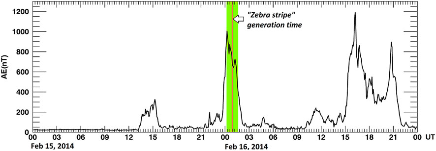
FIGURE 1. The time evolution of the AE index on 15 February 2014 and 16 February 2014. The estimated time for the generation of zebra stripes is indicated by an orange line. The standard deviation of the estimate is shaded in green. A substorm onset occurred during this time interval, at 00:15 UT on 16 February 2014 according to the criteria set by Newell and Gjerloev (2011).
The mostly quiet AE values of 15 February 2014 and the fast variations measured around substorm onset indicates that the main source of electric field disturbances for this event is the prompt penetration of magnetospheric convection.
2.3 Relating Measured Fluctuations in Trapped Particles’ Directional Differential Fluxes and Radial Transport
Sudden variations of the fields produce drift echoes (e.g., Lanzerotti et al., 1967), that is, drift-periodic fluctuations in flux measurements. The amplitude of the fluctuation is related to the radial transport for trapped populations below
where
Where
• There is no significant source or loss mechanism on the time scale of many hours (i.e. multiple drift periods), so that the phase space density
• The timescale for electric field variations is such that the drift motion is the only perturbed motion: in other words, the first and second adiabatic invariants are conserved;
• There is no time variation of the magnetic field and the magnetic field is mainly dipolar.
2.4 Data Set and Data Processing
2.4.1 Van Allen Probes Data Set
We analyze directional differential fluxes between
The Van Allen Probes had a perigee at ∼
2.4.2 Data Processing
To compute the fluctuations in directional differential fluxes,
Figure 2 shows the equatorial electron intensity at L = 1.8 during two successive inbound crossings on 16 February 2014 at 06:14 UT for Van Allen Probes B (18:14 MLT) and at 08:17 UT for Van Allen Probes A (18:23 MLT). The reference equatorial electron intensity,
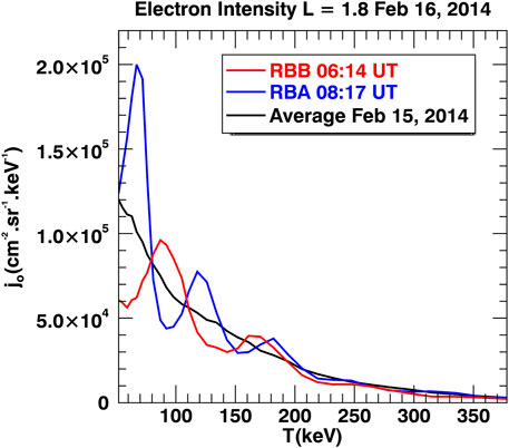
FIGURE 2. Zebra stripes observed during two successive inbound crossings of L = 1.8 (18 MLT), at 06:14 UT by Van Allen Probes B (RBB, in red) and at 08:17 UT by Van Allen Probes A (RBA, in blue). The time-varying equatorial electron intensity is compared with the average equatorial intensity at
3 Results
3.1 Radial Transport From the Analysis of the Zebra Stripes
Figure 3 illustrates how (Section 2.3) information on trapped particles’ radial transport can be retrieved from an analysis of fluctuations in directional differential fluxes observed at a later time. The fluxes are similar to the ones shown in Figure 2. The fluctuations (Figure 3A) are divided by the function
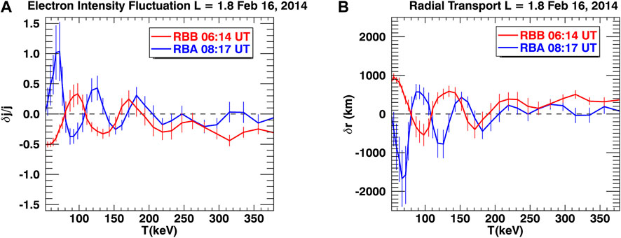
FIGURE 3. (A) Electron intensity fluctuations,
The approach illustrated in Figure 3 is applied to all inbound and outbound crossings of the inner belt and slot region during the morning of 16 February 2014. Figure 4A shows how radial transport generated multiple (∼7) hours before observations is determined from an analysis of fluxes measured during one crossing of 1.5 < L < 2.5. The illustration is for trapped particles with a cosine of the equatorial pitch angle,
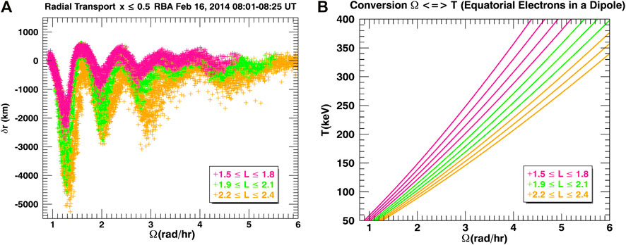
FIGURE 4. (A) Radial transport,
Figure 4A shows how radial transport oscillates with angular drift frequency,
The radial transport estimates shown in Figure 4 as a function of the angular drift frequency do not oscillate symmetrically around a value of zero: They are negative (i.e. inward) on average. One possible interpretation of this observation is that the drift motion of the trapped particles has also been altered by a slower (occurring on a time scale greater than trapped particles’ drift periods) variation of the electric fields. A slow inward transport of the trapped particles requires a relatively steady westward component for the time varying electric fields (Eq. 3). This could be due to the disturbance dynamo action of the storm time winds for instance.
We further investigate the dependence of radial transport with equatorial radial distance,
The estimates for the
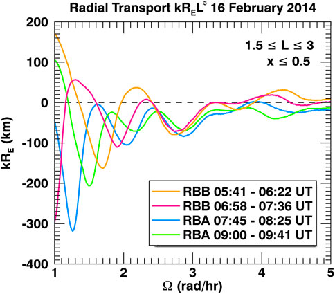
FIGURE 5. Radial transport,
3.2 Radial Transport at L = 1 From Particle Tracing
We apply the model developed by Fejer and Scherliess to compute the perturbation in radial motion (i.e., the ionospheric meridional drift disturbance) based on the time history of the AE index. According to the model, the prompt penetration electric fields are by far the main contributors to the perturbation in radial motion (Section 2.2). The spatial and temporal variations of the electric drift associated with prompt penetration of magnetospheric dynamo electric field is represented in Figure 6. The time interval is from 15 February 2014, 22 UT to 16 February 2014, 10 UT. The sharp increase in the AE index at the beginning of 16 February 2014 is associated with a strong inward motion around 5 MLT (with a maximum magnitude of ∼ −30 m/s). Similarly, the sharp decrease in AE index around two UT is associated with a strong outward motion around 5 MLT (with a maximum magnitude of 24 m/s, i.e., 0.6 mV/m). In comparison, the perturbation in radial motion velocity associated with the disturbance dynamo remains smaller than 6 m/s (0.15 mV/m) throughout the same time interval. With this model, the characteristic time for the variation of the fields is shorter than the drift period (<1 h vs.
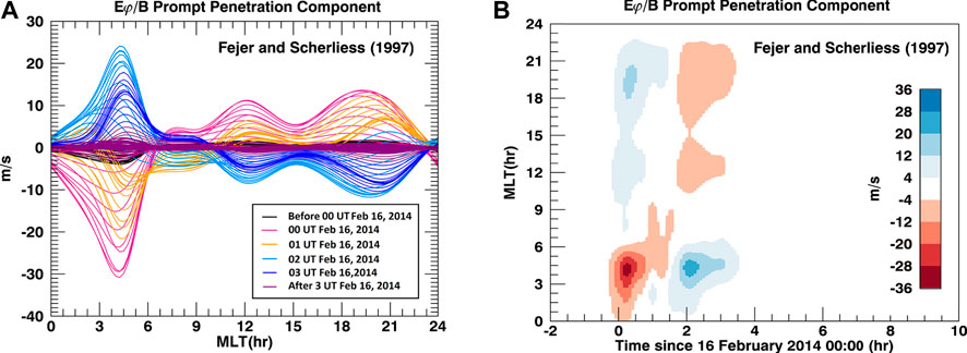
FIGURE 6. 12 h of radial drift motion driven by the prompt penetration of magnetospheric convection between 15 February 2014, 22 UT and 16 February 2014, 10 UT, according to the analytical empirical model developed by Fejer and Scherliess (1997). (A) The amplitude is represented as a function of magnetic local time, MLT, for different times. (B) The amplitude is color-coded as a function of the number of hours since 16 February 2014, 00 UT and the magnetic local time, MLT.
We use these outputs to solve the dynamics of particles unrealistically trapped at L = 1. Using Eq. 3, we launch particles with different angular drift velocities,
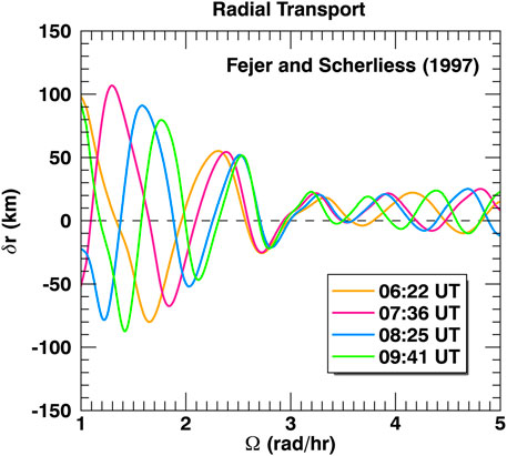
FIGURE 7. Radial transport modeled at L = 1, at the time and magnetic local time zones of Van Allen probes’ crossings (i. e. 5-8 MLT for the inbound passes at 06:22 UT and 08:25 UT and 16–19.5 MLT for the outbound passes at 07:36 UT and 09:41 UT). The electric field disturbances are provided by the analytical empirical formula of Fejer and Scherliess (1997).
The radial transport computed using the modeled electric field disturbances (prompt penetration and disturbance wind dynamo) varies as expected with time, magnetic local time, and angular drift velocity,
3.3 Model-Observation Comparison
The comparison of Figure 5 and Figure 7 shows that the local minima and maxima seen in the experimental estimates for radial transport correspond to the ones obtained numerically. The Pearson correlation coefficient, cc, between the two series (experimental and numerical estimates of radial transport) is high during the first pass, and then decreases with time (06:22UT cc = 0.76; 07:36 UT cc = 0.52; 08:25 UT cc = 0.49; 09:41 UT cc = 0.39). The good agreement between the locations of the extrema and the similitude in the overall shapes of the envelopes suggest that the timing for electric field variations provided by the model is valid for studying radial transport in the inner belt and slot region. On the other hand, the amount of radial transport provided by the model (Figure 7) is smaller than the one resulting from the extrapolation of radial transport experimental estimates down to L = 1 (Figure 5), by approximately a factor 2–3. Because the numerical model comes from an average over many scenarios, it is possible that the penetration electric fields are underestimated in this case. Another difference is that the experimental estimates for radial transport are predominantly negative while the numerical estimates oscillate around zero. This negative offset is present during both inbound passes in the dusk sector and outbound passes in the dawn sector. This rules off the quiet time wind dynamo as the cause of the offset, since the effect of the quiet time wind dynamo depends on local time. Even though the effect of the electric fields due to the disturbance wind dynamo are taken into account in the particle tracing, this discrepancy suggests that their effect is greater than predictions. It could be that the effect of the dynamo electric fields increases with equatorial radial distance in the magnetosphere.
4 Discussion
4.1 Comparing With Radial Transport Based on the Electric Field Dynamics Provided by the Rice Convection Model
We further investigate the model-data discrepancies by running the University of Colorado’s version of the standalone Rice Convection Model (RCM) for 15–16 February 2014 (e.g, Maruyama et al., 2011). The data gaps in the OMNI solar wind parameters are filled using WIND measurements. The modeled prompt penetration electric fields are provided at 100 km altitude, and they are mapped to the magnetic equator assuming equipotential field lines in a magnetic dipole (e.g., Lejosne and Mozer, 2016). Specifically, for the azimuthal electric field component:
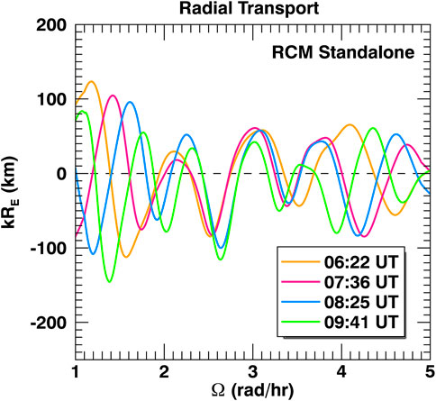
FIGURE 8. Radial transport modeled at L ∼ 1, at the time and magnetic local time zones of Van Allen probes’ crossings (i. e. 5-8 MLT for the inbound passes at 06:22 UT and 08:25 UT and 16–19.5 MLT for the outbound passes at 07:36 UT and 09:41 UT). The electric field disturbances are provided by the standalone version of RCM at L = 1.03.
The quality of the agreement between model and data is lesser here than in Section 3.3, with correlation coefficients below 0.5 in all passes (06:22UT cc = 0.38; 07:36 UT cc = 0.35; 08:25 UT cc = 0.42; 09:41 UT cc = 0.14). That the amplitude of radial transport does not decrease with the angular drift frequency indicates that the characteristic timescale for the variations of the field is faster than the drift period in all cases. This is in contrast with the experimental result, where radial transport decreases and reaches values of the order of a few tens of kilometers for
We leverage the fact that RCM informs on electric field dynamics at all magnetic latitudes to determine the power of L,
4.2 Other Considerations
4.2.1 Instrument Resolution
An instrument with a high-energy resolution is required when it comes to resolving and analyzing drift echoes such as the zebra stripes (e.g., Hartinger et al., 2018). Particles with slightly different kinetic energies sharing the same energy channel will have mixed adiabatically on a time scale of the order of
4.2.2 Radial Diffusion in the Inner Belt and Slot Region
The power of
Data Availability Statement
Publicly available datasets were analyzed in this study. This data can be found here: http://rbspice.ftecs.com/Data.html (RBSPICE database). Simulation outputs can be obtained by contacting NM.
Author Contributions
The first author is the lead and corresponding author. All other authors are listed in alphabetical order. We describe contributions to the paper using the CRediT (Contributor Roles Taxonomy) categories (Brand et al., 2015). Conceptualization, Formal Analysis, Writing—Original Draft, Visualization and Project Administration: SL Funding acquisition, Methodology: SL and NM Resources, Software: SL, BF, NM, and LS. Investigation: SL, BF and LS. Writing-Review & Editing: SL, BF, NM and LS.
Funding
SL work was performed under NASA Grant Awards 80NSSC18K1223 and 80NSSC20K1351. The work of BF was supported by the NASA H-LWS program through grant 80NSSC17K71.
Conflict of Interest
The authors declare that the research was conducted in the absence of any commercial or financial relationships that could be construed as a potential conflict of interest.
Publisher’s Note
All claims expressed in this article are solely those of the authors and do not necessarily represent those of their affiliated organizations, or those of the publisher, the editors and the reviewers. Any product that may be evaluated in this article, or claim that may be made by its manufacturer, is not guaranteed or endorsed by the publisher.
Acknowledgments
The use of OMNI data and NASA/GSFC’s Space Physics Data Facility’s OMNIWeb (https://omniweb.gsfc.nasa.gov/) service is acknowledged. We also acknowledge the substorm timing list identified by the Newell and Gjerloev technique (Newell and Gjerloev, 2011a), the SMU and SML indices (Newell and Gjerloev, 2011b); and the SuperMAG collaboration (Gjerloev, 2012). SL thanks C. Huang for a helpful discussion about ionospheric E-field measurements. SL and NM thank Mariangel Fedrizzi for a helpful discussion about filling data gaps in solar wind measurements.
References
Brand, A., Allen, L., Altman, M., Hlava, M., and Scott, J. (2015). Beyond Authorship: Attribution, Contribution, Collaboration, and Credit. Learn. Pub. 28, 151–155. doi:10.1087/20150211
Fälthammar, C.-G. (1965). Effects of Time-Dependent Electric fields on Geomagnetically Trapped Radiation. J. Geophys. Res. 70 (11), 2503–2516. doi:10.1029/JZ070i011p02503
Fälthammar, C.-G. (1968). “Radial Diffusion by Violation of the Third Adiabatic Invariant,” in Earth's Particles and fields. Editor B. M. McCormac (New York: Reinhold), 157–169.
Fejer, B. G., and Scherliess, L. (1995). Time Dependent Response of Equatorial Ionospheric Electric fields to Magnetospheric Disturbances. Geophys. Res. Lett. 22 (7), 851–854. doi:10.1029/95GL00390
Fejer, B. G., and Scherliess, L. (1997). Empirical Models of Storm Time Equatorial Zonal Electric fields. J. Geophys. Res. 102 (A11), 24047–24056. doi:10.1029/97JA02164
Fejer, B. G., Blanc, M., and Richmond, A. D. (2017). Post-Storm Middle and Low-Latitude Ionospheric Electric Fields Effects. Space Sci. Rev. 206, 407–429. doi:10.1007/s11214-016-0320-x
Gjerloev, J. W. (2012). The SuperMAG Data Processing Technique. J. Geophys. Res. 117, A09213. doi:10.1029/2012JA017683
Hartinger, M. D., Claudepierre, S. G., Turner, D. L., Reeves, G. D., Breneman, A., Mann, I. R., et al. (2018). Diagnosis of ULF Wave‐Particle Interactions with Megaelectron Volt Electrons: The Importance of Ultrahigh‐Resolution Energy Channels. Geophys. Res. Lett. 45, 11,883–11,892. doi:10.1029/2018GL080291
Imhof, W. L., and Smith, R. V. (1965). Observation of Nearly Monoenergetic High-Energy Electrons in the Inner Radiation Belt. Phys. Rev. Lett. 14, 885–887. doi:10.1103/PhysRevLett.14.885
Lanzerotti, L. J., Roberts, C. S., and Brown, W. L. (1967). Temporal Variations in the Electron Flux at Synchronous Altitudes. J. Geophys. Res. 72 (23), 5893–5902. doi:10.1029/JZ072i023p05893
Lejosne, S., and Mozer, F. S. (2016). Typical Values of the Electric Drift E × B/B 2 in the Inner Radiation belt and Slot Region as Determined from Van Allen Probe Measurements. J. Geophys. Res. Space Phys. 121, 12014–12024. doi:10.1002/2016JA023613
Lejosne, S., and Mozer, F. S. (2018). Magnetic Activity Dependence of the Electric Drift below L = 3. Geophys. Res. Lett. 45, 3775–3782. doi:10.1029/2018GL077873
Lejosne, S., and Mozer, F. S. (2020a). Experimental Determination of the Conditions Associated with "Zebra Stripe" Pattern Generation in the Earth's Inner Radiation Belt and Slot Region. J. Geophys. Res. Space Phys. 125, e2020JA027889. doi:10.1029/2020JA027889
Lejosne, S., and Mozer, F. S. (2020b). Inversion of the Energetic Electron "Zebra Stripe" Pattern Present in the Earth's Inner Belt and Slot Region: First Observations and Interpretation. Geophys. Res. Lett. 47, e2020GL088564. doi:10.1029/2020GL088564
Lejosne, S., and Roederer, J. G. (2016). The “Zebra Stripes”: An Effect of F Region Zonal Plasma Drifts on the Longitudinal Distribution of Radiation belt Particles. J. Geophys. Res. Space Phys. 121, 507–518. doi:10.1002/2015JA021925
Lejosne, S., Fedrizzi, M., Maruyama, N., and Selesnick, R. S. (2021). Thermospheric Neutral Winds as the Cause of Drift Shell Distortion in Earth's Inner Radiation Belt. Front. Astron. Space Sci. 8, 725800. doi:10.3389/fspas.2021.725800
Liu, Y., Zong, Q.-G., Zhou, X.-Z., Foster, J. C., and Rankin, R. (2016). Structure and Evolution of Electron “Zebra Stripes” in the Inner Radiation belt. J. Geophys. Res. Space Phys. 121, 4145–4157. doi:10.1002/2015JA022077
Maruyama, N., Fuller‐Rowell, T. J., Codrescu, M. V., Anderson, D., Richmond, A. D., Maute, A., et al. (2011). “Modeling the Storm Time Electrodynamics,” in Aeronomy of the Earth's Atmosphere and Ionosphere, IAGA Special Sopron Book Series. Editors M. Abdu, and D. Pancheva (Dordrecht: Springer), 2, 455–464. doi:10.1007/978‐94‐007‐0326‐1_35
Mauk, B. H., Fox, N. J., Kanekal, S. G., Kessel, R. L., Sibeck, D. G., and Ukhorskiy, A. (2013). Science Objectives and Rationale for the Radiation Belt Storm Probes Mission. Space Sci. Rev. 179, 3–27. doi:10.1007/s11214-012-9908-y
Mitchell, D. G., Lanzerotti, L. J., Kim, C. K., Stokes, M., Ho, G., Cooper, S., et al. (2013). Radiation Belt Storm Probes Ion Composition Experiment (RBSPICE). Space Sci. Rev. 179, 263–308. doi:10.1007/s11214-013-9965-x
Mozer, F. S. (1970). Electric Field Mapping in the Ionosphere at the Equatorial Plane. Planet. Space Sci. 18, 259–263. doi:10.1016/0032-0633(70)90161-3
Newell, P. T., and Gjerloev, J. W. (2011a). Evaluation of SuperMAG Auroral Electrojet Indices as Indicators of Substorms and Auroral Power. J. Geophys. Res. 116, A12211. doi:10.1029/2011JA016779
Newell, P. T., and Gjerloev, J. W. (2011b). Substorm and Magnetosphere Characteristic Scales Inferred from the SuperMAG Auroral Electrojet Indices. J. Geophys. Res. 116, A12232. doi:10.1029/2011JA016936
Richmond, A. D., Blanc, M., Emery, B. A., Wand, R. H., Fejer, B. G., Woodman, R. F., et al. (1980). An Empirical Model of Quiet-Day Ionospheric Electric Fields at Middle and Low Latitudes. J. Geophys. Res. 85, 4658–4664. doi:10.1029/JA085iA09p04658
Roederer, J. G., Hilton, H. H., and Schulz, M. (1973). Drift Shell Splitting by Internal Geomagnetic Multipoles. J. Geophys. Res. 78 (1), 133–144. doi:10.1029/JA078i001p00133
Sandel, B. R., Goldstein, J., Gallagher, D. L., and Spasojevic, M. (2003). Extreme Ultraviolet Imager Observations of the Structure and Dynamics of the Plasmasphere. Space Sci. Rev. 109, 25–46. doi:10.1023/b:spac.0000007511.47727.5b
Sauvaud, J.-A., Walt, M., Delcourt, D., Benoist, C., Penou, E., Chen, Y., et al. (2013). Inner Radiation belt Particle Acceleration and Energy Structuring by Drift Resonance with ULF Waves during Geomagnetic Storms. J. Geophys. Res. Space Phys. 118, 1723–1736. doi:10.1002/jgra.50125
Schulz, M., and Lanzerotti, L. J. (1974). Particle Diffusion in the Radiation Belts. Berlin, Heidelberg: Springer-Verlag. doi:10.1007/978-3-642-65675-0
Selesnick, R. S., Su, Y. J., and Blake, J. B. (2016). Control of the Innermost Electron Radiation belt by Large‐scale Electric fields. J. Geophys. Res. Space Phys. 121, 8417–8427. doi:10.1002/2016JA022973
Sun, Y. X., Roussos, E., Hao, Y. X., Zong, Q.-G., Liu, Y., Lejosne, S., et al. (2021). Saturn's Inner Magnetospheric Convection in the View of Zebra Stripe Patterns in Energetic Electron Spectra. J. Geophys. Res. Space Phys. 126, e2021JA029600. doi:10.1029/2021ja029600
Tsyganenko, N. A. (1989). A Magnetospheric Magnetic Field Model with a Warped Tail Current Sheet. Planet. Space Sci. 37 (1), 5–20. doi:10.1016/0032-0633(89)90066-4
Keywords: radial transport, prompt penetration electric fields, disturbance electric fields, trapped particles, Earth’s inner radiation belt, van allen probes
Citation: Lejosne S, Fejer BG, Maruyama N and Scherliess L (2022) Radial Transport of Energetic Electrons as Determined From the “Zebra Stripes” Measured in the Earth’s Inner Belt and Slot Region. Front. Astron. Space Sci. 9:823695. doi: 10.3389/fspas.2022.823695
Received: 28 November 2021; Accepted: 13 January 2022;
Published: 17 February 2022.
Edited by:
Jean-Francois Ripoll, CEA DAM Île-de-France, FranceReviewed by:
Theodore Sarris, Democritus University of Thrace, GreeceClare Watt, Northumbria University, United Kingdom
Copyright © 2022 Lejosne, Fejer, Maruyama and Scherliess. This is an open-access article distributed under the terms of the Creative Commons Attribution License (CC BY). The use, distribution or reproduction in other forums is permitted, provided the original author(s) and the copyright owner(s) are credited and that the original publication in this journal is cited, in accordance with accepted academic practice. No use, distribution or reproduction is permitted which does not comply with these terms.
*Correspondence: Solène Lejosne, c29sZW5lQGJlcmtlbGV5LmVkdQ==