 Julie Hartz
 Simon C. George
94% of researchers rate our articles as excellent or good
Learn more about the work of our research integrity team to safeguard the quality of each article we publish.
Find out more
BRIEF RESEARCH REPORT article
Front. Astron. Space Sci. , 14 March 2022
Sec. Astrobiology
Volume 9 - 2022 | https://doi.org/10.3389/fspas.2022.769607
In July 2020, NASA’s Perseverance (Mars 2020) mission was launched. The rover sent to the surface of Mars will not only perform in situ analyses, but will also collect rock and regolith samples that will be returned to Earth by future missions for further investigations. Therefore, the amount and quality of astrobiological data retrieved from these missions is expected to be unprecedented. The challenge faced by the astrobiology community will be to use these data in the most efficient way to assess whether any of the analysed samples are of biogenic origin. However, in situ biogenic assessments often lack quantitative support. Particularly, their statistical uncertainty is not systematically evaluated. This study aims to provide the first quantitative framework that evaluates the uncertainty of in situ biogenic assessments using recursive Bayesian statistics. Our results show that detecting more than seven potential biosignatures does not increase the reliability of biogenic assessments, unless the probability of detection of biosignatures in the sample and the probability of the biosignatures being false positives are well constrained. This study emphasizes the need for quantitative support of biogenic assessments and astrobiology strategies in general.
Modern analytical techniques allow the astrobiology community to detect a great diversity of potential biosignatures that may be preserved in the geological record, and may provide evidence for the earliest traces of life on Earth and for traces of extra-terrestrial life in other planetary systems. Six different types of in situ biosignatures have been defined by the MARS 2020 Science Definition Team (Hays et al., 2017): 1) macro- and 2) micro-structures, 3) minerals, 4) organics, 5) chemistry, and 6) isotopes. While some potential biosignatures unequivocally indicate a biological origin, the DNA molecule for example, others are less tangible proof of life on which biogenic assessments cannot solely rely, such as micro-stromatolitic textures. Some potential biosignatures are easier to detect than others, for example detecting complex organic compounds requires advanced analytical techniques, whereas macrofossils are identifiable by the naked eye. Also, potential biosignatures are not equally preserved through time in the geological record. Some tend to be degraded, or even lost, during diagenesis and metamorphism, while others remain at least quasi-intact for billions of years. Hence, it appears that potential biosignatures may be ranked according to three criteria: their reliability (i.e., the probability of a biosignature to be produced by life), their detectability (i.e., the likelihood that a biosignature can be observed or measured), and their survivability (i.e., their ability to be preserved in the geological record) (The National Academies of Sciences, Engineering, and Medicine, 2018). Therefore, despite modern advances in analytical techniques, assessing the unequivocal biogenicity of a rock sample remains challenging and controversial.
On Earth, evidence for ancient life forms is often questioned as new data is collected from additional analyses. For example, biogenic assessments relying on Archean microfossils are often re-evaluated as new geochemical data are collected (e.g. Archean stromatolites from the Apex Chert, Pilbara, Australia: Altermann and Kazmierczak, 2003; Brasier et al., 2006). On Mars, most biological experiments conducted by previous missions have been inconclusive, despite a growing number of potential biosignatures detected on the Martian surface. For example, while the Viking Labeled release experiment returned positive results for metabolic activity on the surface of Mars (Levin, 1972; Levin and Straat, 2016), the scientific community could not rule out an abiological origin for the presumed metabolic oxidants detected in the Martian soil (Klein, 1999). Therefore, it appears that the uncertainty of biogenic assessments prevents the astrobiology community to come to a consensus regarding Earth’s oldest life forms and Mars’ past biological activity.
To address this issue and strengthen the reliability of biogenic assessments, most recent astrobiology strategies are focussed on three topics: 1) identifying novel biosignatures, 2) identifying abiotic processes that may mimic biosignatures, and 3) better constraining the preservation pathways of currently known biosignatures. However, it is unclear whether all three topics are equally important for biogenic assessments. Would increasing the number of potential biosignatures increase the reliability of the biogenic assessments? Or should a biogenic assessment consider fewer but better constrained biosignatures? Elements of answers to these questions may provide quantitative guidelines for the search for the oldest life forms on Earth and for remnants of extraterrestrial life on other planetary bodies. Also, while efforts have been made to qualitatively assess the reliability of biogenic assessments (e.g. The Ladder of Life Detection, Neveu et al., 2018), limited efforts have been put to statistically quantify the uncertainty of biogenic assessments. Catling et al. (2018) developed a Bayesian approach to identify the information and procedures required to quantify the confidence that a potential biosignature, namely spectral and photometric signals, detected on an exoplanet is truly a detection of life. Similarly, Walker et al. (2018) introduced a Bayesian method for guiding future directions for detection of life on exoplanets. While Catling et al. (2018) focuses on the biogeochemistry of exoplanets as recorded by atmospheric signatures, Walker et al. (2018) advocates for a Bayesian method spanning a wide range of potential biosignatures derived from various definitions of life. Bayesian statistics have also proved useful to quantify the probability of success of space missions (Sephton and Carter, 2015). The present study aims to provide a quantitative framework that evaluates the uncertainty of in situ biogenic assessments using a simple Bayesian inference. More sophisticated Bayesian methods allow for more accurate estimations and decision-making in astrobiology in the presence of instrumental and processing noise and multiple sources of uncertainty, such as Bayesian networks or Kalman filter (Ellery, 2018; Dai et al., 2019). We find that detecting more than seven potential biosignatures does not increase the reliability of biogenic assessments, unless their probability of being false positives is well constrained.
To ensure this article is accessible to a wide audience, the following statistical model is described assuming relatively little familiarity with Bayesian statistics.
Bayesian methods are founded on the explicit use of judgement, expressed as prior beliefs, and provide a natural means of revising opinions in the light of new evidence. As opposed to frequentist statistical approaches, Bayesian frameworks are agnostic to any pre-specified sample size (Spiegelhalter et al., 2004). Therefore, a Bayesian statistical approach would be particularly useful when assessing if an astrobiological sample is biogenic, given the low number of tests that can be performed on the sample due to space missions’ limitations (i.e. mission payload, instrument limitations, etc). One way of formulating Bayes’ theorem is as follows:
where P (A|B) is the probability of the hypothesis A to be true given the evidence B and is called the “posterior” probability, P(B|A) is the likelihood of the evidence B to occur if the hypothesis A is true, P(A) is the initial degree of belief that the hypothesis A is true and is called the “prior” probability, P(B|
One of many applications of Bayes’ theorem is the Bayesian inference, when Bayes’ rule is repeatedly applied as new data is collected from the same object, or as new tests are performed on the same object, in order to determine whether the hypothesis about the object is true. For example, a patient who shows symptoms for a specific disease would consult a doctor who would perform a series of tests in order to determine whether the patient contracted the disease or not. Each test is characterised by a probability of being positive if the patient is sick and by a probability of being a false positive. The prior probability is determined by the initial belief of the patient being sick and was assessed based on the patient’s symptoms. If a first test returns negative, the posterior probability that the patient is sick is lower than the initial prior probability. The initial belief is then updated after the first data were collected. Then a second test is performed, also returning negative. The prior probability used for this second assessment is the posterior probability that was updated after the first test, and so on. Mathematically, the Bayesian inference may be formulated as follows:
where n (n ≥ 1) is the number of tests performed, and i (1 ≤ i ≤ n) is the ith test. It is important to note that the sample always remains the same, only the tests differ.
A key question in Bayesian analysis is the choice of the prior as it sets the starting point of the inference procedure. A prior can be 1) “informative” when it expresses specific information about a variable, 2) “weakly informative” when it expresses partial information, or 3) “diffuse” when very little to no information is expressed. “Informative” and “weakly informative” priors tend to reflect higher levels of subjectivity. A researcher may have a very strong, yet educated, opinion about the model parameter values that may drive and eventually bias the final model estimates (Depaoli et al., 2017; van de Schoot et al., 2018). In contrast, “diffuse” priors tend to be more objective, or at least express objective information about a variable. Nonetheless, “diffuse” priors have their own limitations and may not always be a viable option (Natarajan and McCulloch, 1998; Van Erp et al., 2018). To assist in the choice of the prior, it has been recommended to always conduct a sensitivity analysis of priors, by examining the final model results obtained from different priors (Muthén and Asparouhov, 2012). In this study, the Bayesian inference will make use of a “diffuse” prior that reflects a specific situation in astrobiology that is discussed in the next section.
Based on Bayes’ theorem, the statistical model developed in Catling et al. (2018) is of particular relevance as it evaluates the likelihood of an exoplanet to be hosting life, given the potential biosignatures collected and the exoplanetary context. The model is formulated as follows:
where P (life|D,C) is the probability of an exoplanet to host life given the data collected D and the exoplanetary context C, P (D|C,life) is the likelihood of the data D to occur in that exoplanetary context C if there is life, P (D|C, no life) is the likelihood of the data D to occur in that exoplanetary context C if life is not present (i.e., the likelihood of being a false positive), and P (life|C) and P (no life|C) are the likelihoods of life being present and not present, respectively, in that exoplanetary context C (i.e., the prior probabilities). Assuming that the hypothesis of an exoplanet to host life is binary, either life is present on the exoplanet or not, the two prior probabilities of life being present, P (life|C), and of life not being present, P (no life|C), are complementary and related by P (life|C) = 1-P (no life|C). Applied to in situ biosignatures and biogenic assessments of fossil sinters, and of the geological record in general, Eq. 3 can be re-formulated as follows:
Where the term signature refers to a potential biosignature (i.e. a biosignature or a false positive signature), P (biogenic|signature,C) is the posterior probability of a sample to be biogenic given the signature detected in the sample’s context C, P (signature|C, biogenic) is the likelihood of the signature to occur in that sample’s context C if it is biogenic, P (biogenic|C) is the prior probability of the sample to be biogenic given its context (i.e., the prior probability), and P (signature|C, abiogenic) is the likelihood of the signature to occur in the sample if it is not biogenic (i.e., the likelihood of being a false positive).
Similarly to the medical example described above, a set of potential biosignatures detected in a rock sample can be considered as a series of tests that are performed on the rock sample to determine whether it is biogenic or not. Figure 1 illustrates the process of Bayesian inference in an astrobiological context. Each potential biosignature has a specific likelihood to be detected in the sample and a specific probability of being a false positive. Therefore, a Bayesian inference applied to Eq. 4 may be formulated as follows:
where n (n ≥ 1) is the number of signatures detected in the sample, and i (1 ≤ i ≤ n) is the ith signature. Here again, while the signatures detected in the sample may differ, the sample itself always remains the same. For n = 1, P (biogenic|C)0 is the initial prior probability determined by the prior knowledge of the habitability of the sample’s depositional environment. From Eq. 5, biogenic assessments rely on three variables: (i) P (signature|C,biogenic)i, the likelihood of each signature to occur in the sample if it is biogenic; (ii) P (biogenic|C)n-1, the prior knowledge of the habitability of the sample’s depositional environment; and (iii) P (signature|C,abiogenic)i, the likelihood of each signature of being a false positive.
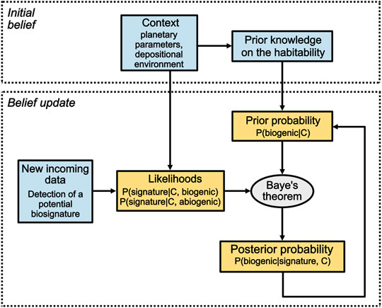
FIGURE 1. The Bayesian model developed in this study may assist in assessing the biogenicity of extraterrestrial samples in a similar way to the medical example provided in Section 2.1. Consider NASA’s Perseverance (MARS 2020) mission as an example. Jezero Crater has been chosen as the mission landing site due to its likelihood to having been habitable, among other geological and engineering criteria. The initial belief about Jezero Crater’s habitability represents the initial belief that a sample collected within the crater is biogenic and is formulated as P (biogenic|C)0. If a first potential biosignature is detected by one of Perseverance’s instruments within a sample, the likelihood of the biosignature to occur given the context if the sample is biogenic P (signature|C, biogenic) and abiogenic P (signature|C, abiogenic) can be determined, or at least estimated. Using Baye’s theorem, the posterior probability of the sample being biogenic given the potential biosignature detected and the planetary context, P (biogenic|signature, C), can now be computed. If a second potential biosignature is detected within the same sample, a new Bayesian inference begins using the previous posterior probability as the updated prior probability. The number of inferences is determined by the number of potential biosignatures detected. Blue boxes contain data and yellow boxes contain probabilities inferred from these data.
The prior designates the initial degree of belief that the sample is biogenic, given its context before any data was collected. This initial belief reflects our combined knowledge about the sample’s planetary, environmental, and geological context, as well as our knowledge about life, its potential origins, emergence processes, and survival limits. For example, on a planetary scale, Mars has been the predominant astrobiological target in our Solar System, because in its early history, the planetary and environmental conditions might have been similar, to some extent, to those of early Earth’s (Sautter et al., 2015; McLennan et al., 2019). Considering that some of the earliest traces of life on Earth are around 3.5 Byrs old (Djokic et al., 2017; Dodd et al., 2017), it is fair to hypothesize that life could have been present on Mars around the same time. On an environmental scale, Jezero Crater was selected as NASA’s Perseverance (Mars 2020) mission landing site, from 60 other candidates, because previous investigations indicated that the area must have undergone wetting-drying cycles in the early history of Mars. Wetting-drying cycles have been shown to enable the polymerization of complex biomolecules including the building blocks of life (Mulkidjanian et al., 2012a; Mulkidjanian et al., 2012b; Stüeken et al., 2013).
The above contextual information about Jezero Crater determines the prior probability of a sample from that area to be biogenic. However, as mentioned in Section 2.1, in Bayesian analysis the prior tend to reflect a subjective belief that not everybody might subscribe to. In fact, many scientists advocated for Columbia Hills as NASA’s Perseverance landing site, because they believe that hot springs are more suitable environments for life to emerge and be sustained (Squyres et al., 2008; Ruff et al., 2011; Teece et al., 2020).
Here, we chose a “diffuse” prior, specifically a “uniform” prior (i.e. following a uniform distribution), so as to reflect no previous knowledge about the potential biogenicity of a sample. While diffuse priors may bypass the subjective component of the Bayesian analysis, it is important to notice that setting the prior to be uniform only captures a very specific situation, that nothing is known about the system’s context. In astrobiological terms, a uniform prior reflects the situation where we do not know anything about a sample’s planetary or environmental context. This choice of prior does not reflect a practical situation as expensive and technically challenging astrobiology-focused missions would want to target the best-known relevant environments.
The likelihood term designates the likelihood of the data to be present in the sample, if it is biogenic, and given the sample’s context. In other words, it quantifies the compatibility of the evidence with the hypothesis. The likelihood is a variable of the context of the sample. For example, scientists believe that river channels within the Jezero Crater area might have transported clay minerals into the crater lake (Ehlmann et al., 2008), that would have formed a well-preserved fluvio-deltaic stratigraphy with a high potential to concentrate and preserve organic matter (Goudge et al., 2017). Therefore, detecting organic compounds in samples from Jezero Crater would be consistent with the site’s context. The likelihood is also a variable of instrumental criteria, such as sensitivity, detection limits, and noise. In other words, the likelihood reflects the detectability of a signal.
Finally, the false positive term designates the likelihood of the data to be present in the sample, if it is not biogenic, and given the planetary, geological, and environmental context. It is the probability of the data to be abiotic observations that mimic biologically-produced signals. Such signals may originate from three sources: unknown abiotic processes, contamination, and byproducts. For example, the detection of chlorinated hydrocarbons by NASA’s Curiosity Sample Analysis at Mars (SAM) have been shown to most likely be produced during heating of samples in the presence of chlorinated compounds, rather than to be of a Martian origin (Ming et al., 2014).
Determining the precise value or describing the probability densities of each variable involved in Eq. 5 and for each type of biosignature is beyond the scope of this study. However, understanding the influence of each variable on the final output of Eq. 5 (i.e., the nth posterior probability) is not as tedious and may provide quantitatively-assessed guidelines for current astrobiology strategies.
A common way to evaluate how a model responds to each variable is to perform a sensitivity analysis on that same model. A sensitivity analysis can be used for various objectives, and these should be specified beforehand (Saltelli et al., 2004). These objectives may include: 1) identify and prioritise the most influential inputs; 2) identify non-influential inputs in order to simplify a model (usually for models involving a high number of inputs like ocean circulation models); or 3) calibrate model inputs using the information that is known on the model (e.g., constraints, real output observations, etc...). Here, the sensitivity analysis performed on Eq. 5 has the objective to identify the most influential variables on the model output.
Different levels of sensitivity can be analysed during a sensitivity analysis. Comprehensive reviews of sensitivity analysis techniques are provided in De Rocquigny et al. (2008), Castaings et al. (2009), and Iooss and Lemaître (2015). Given that Eq. 5 only involves three variables, a sensitivity analysis technique that is computationally costly may be considered. Eq. 5 is directly derived from Bayes’ theorem and no prior assumptions are made in order to formulate the end model. Also, no assumptions are made on any of the inputs as each input will be evaluated on the full variation range from 0 to 1. The number of model inputs is low, therefore the computational cost is also low. Therefore, the best suited sensitivity analysis method for Eq. 5 is the Sobol’ indices, or the Sobol’ method (Sobol, 1993; De Rocquigny et al., 2008).
Sobol’ Indices, also called variance-based sensitivity analysis, decompose the variance of a model output into fractions that can be attributed to the variance of the model inputs. Sobol’ indices have become a widely-used variance-based method for sensitivity analysis across various scientific fields (Sobol, 1993). There are several types of Sobol’ indices. The first order Sobol’ sensitivity index accounts for the proportion of variance of a model output explained by changing each variable alone while marginalizing over the rest, and are computed as follows:
Where
While the first order Sobol’ indices may be analytically computed by evaluating the integrals in the decomposition of the variance, in most cases they are estimated. There are various estimators of Sobol’ indices, mostly differing in their sampling procedures and computational costs (Tarantola et al., 2006). Here, the first order Sobol’ indices of Eq. 5 were computed following the Monte Carlo method described in Monod et al. (2006) (Section 4.2.4.2 Estimation based on Monte Carlo sampling) and implemented in the ‘sobolSalt’ function of the R ‘sensitivity’ package (https://cran.r-project.org/web/packages/sensitivity/sensitivity.pdf). The indices were computed along fifteen biosignatures (n = 15), as beyond fifteen Bayesian inferences the results from the sensitivity analysis stabilise (Figure 2). Following Monod et al. (2006)’s procedure, the indices were estimated using
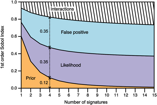
FIGURE 2. Evolution of the first order Sobol’ indices along with the increasing number of signatures for the prior probability (orange area), the likelihood variable (purple area), the false positive variable (blue area), and their interactions (hatched area). The Sobol’ index values of each variable are given by the vertical extent of the colored fields. For example, for n = 4, the prior probability has a first Sobol’ index value of 0.12, whereas the likelihood and false positive variables have first Sobol’ index values of 0.35 each. In other words, when detecting four potential biosignatures, the uncertainty of the prior is responsible for 12% the uncertainty of the biogenic assessment, whereas the uncertainty of the likelihood and false positive are distinctively responsible for 35% of the final assessment’s uncertainty.
The first order Sobol’ indices of each variable were plotted against the increasing number of potential biosignatures n from 1 to 15 (Figure 2). The term “prior” designates the prior knowledge of the sample’s depositional environment, the term “likelihood” designates the likelihood of a potential biosignature to occur in the sample’s depositional environment if it is biogenic, the term “false positive” designates the probability of the potential biosignature to be a false positive (i.e. to occur in the sample’s depositional environment if it is not biogenic), and the term “posterior” designates the output probability of the sample to be biogenic given the potential biosignatures detected and the sample’s depositional environment.
For a single potential biosignature (n = 1), the prior probability has a first order index of 0.6, while the likelihood and the false positive have first order indices of ∼0.16 and ∼0.17, respectively. Therefore, for a single potential biosignature, the prior’s variance is responsible for 60% of the posterior’s variance, whereas the likelihood’s and false positive’s variances are responsible for 16 and 17% of the posterior’s variance, respectively. The remaining 7% of the posterior’s variance is due to variables interacting with each other (Figure 2). In other words, when detecting a single biosignature, 60% of the uncertainty of biogenic assessments comes from the uncertainty of the prior, whereas the uncertainty of the likelihood and false positive are responsible for 16 and 17%, respectively, of the uncertainty of the final biogenic assessment.
As the number of potential biosignatures increases, the first order index of the prior probability strongly decreases until n = 4, before steadily decreasing until its minimal value of 0.01 for n = 15. Conversely, the first order indices of the likelihood and the false positive sharply increase from n = 1 to n = 4, before steadily increasing until their maximal values of 0.35 for n = 15. Therefore, as the number of potential biosignatures increases, the uncertainty of the prior probability sharply decreases, from being responsible for 60% of the posterior’s uncertainty for n = 1, to no more than 1% for n = 15. Moreover, the uncertainties of the likelihood and the false positive sharply increase, from being responsible for 16 and 17% of the posterior’s variance for n = 1, respectively, to as much as 35% for n = 15. Similarly, the effect of the interactions between the three variables smoothly increases, from being responsible for 7% of the posterior’s variance for n = 1, to nearly 26% for n = 15 (Figure 2).
The results of the sensitivity analysis using Eq. 5 show that 60% of the uncertainty of biogenic assessments based on a single potential biosignature is due to the uncertainty of the prior habitability assessment of the sample’s depositional environment. In other words, for a single potential biosignature, knowing the exact probability of the habitability of a sample’s depositional environment would reduce the uncertainty of the final biogenic assessment by 60%.
As new potential biosignatures are detected in the sample, the effect of the habitability of the sample’s depositional environment on the final biogenic assessment sharply decreases, from being responsible for 12% of the uncertainty of the final biogenic assessment for four potential biosignatures, to about 5% for seven potential biosignatures, and finally reaching a minimum value of 1% for 15 potential biosignatures. This result implies that when seven or more potential biosignatures are detected in the sample, knowing the exact probability of the habitability of the sample’s depositional environment will only reduce the uncertainty of the biogenic assessment by 5% or less (i.e. it will only increase the reliability of the biogenic assessment by 5% or less). Therefore, for more than seven potential biosignatures, the effect of the habitability of the sample’s depositional environment on the final biogenic assessment becomes negligible. These results are in accordance with the recursive Bayesian inference whose purpose is to update the prior belief of a hypothesis to be true as new data are collected, so that it has a negligible influence on the end output. Therefore, this result shows that the Sobol’ method is consistent with the model expressed by Eq. 5.
Conversely, the uncertainty of the likelihood of a potential biosignature to occur in a biogenic sample and its probability of being a false positive is increasingly responsible for the uncertainty of the final biogenic assessment when there are greater numbers of potential biosignatures. For four potential biosignatures, both parameters have already reached their maximum influence on the biogenic assessment and are equally responsible for 35% of the biogenic assessment’s uncertainty. This implies that knowing the exact probability of a potential biosignature to occur in a biogenic sample and to be a false positive would increase the reliability of biogenic assessments by nearly 70%.
The combination of these results has implications for astrobiological strategies. Firstly, the reliability of biogenic assessments based on a single potential biosignature mainly relies on our understanding of the sample’s depositional environment. Secondly, detecting four or more potential biosignatures does not increase the reliability of biogenic assessments unless the processes forming, preserving, and mimicking those biosignatures are well-constrained. Thirdly, for more than seven biosignatures, the importance of our prior understanding of the sample’s depositional environment is negligible.
However, there are several significant limitations to the approach presented here. As mentioned in Section 2.3, performing the Sobol’ method on a model requires the model inputs to be independent and non-correlated and the model to be deterministic. In Eq. 5, it is most likely that P (biosignature|C,biogenic)i, the likelihood of the ith biosignature to occur in a biogenic sample, is at least partly determined by P (biogenic|C)0, the prior knowledge of the habitability of the sample’s depositional environment. For example, the likelihood of detecting signs of oxygen-consuming organisms is much lower for samples collected on the surface of Titan that has an atmosphere mainly composed of nitrogen and methane, than on the surface of Earth where atmospheric oxygen is abundant. However, the dependence issue is addressed by the random sampling method. As a fixed value is randomly attributed to each variable prior to the calculation of the Sobol’ indices, the dependent relationship between the variables is eliminated. Moreover, to date there is no mathematical correlation in the literature that links the habitability of an environment with the likelihood of a biosignature to occur in that same environment. However, such correlation is not completely implausible and the fact that it has not been documented does not refute its existence. Nevertheless, even if at least two variables in Eq. 5 were correlated, the random sampling method would also eliminate any sense of correlation between the variables. In summary, the stochastic model from which Eq. 5 is derived (i.e., the Bayesian inference) is simplified to a deterministic model by attributing randomly pre-determined values to each variable. Therefore, the random sampling method enables the computation of Sobol’ indices for Eq. 5 but is not a high-fidelity representation of the natural processes involved in the formation, preservation, and detection of biosignatures.
Also, while the model quantitatively evaluates the uncertainty of biogenic assessments, we realize that its practical implementation is challenging when looking for life in a relatively unknown and inaccessible environment, such as Mars for instance. The diversity and variability of the environmental conditions make it difficult to accurately estimate the values of the likelihoods of biosignatures to occur and to be false positives. However, tools like The Ladder of Life Detection (Neveu et al., 2018) or other Bayesian frameworks developed for exoplanetary biosignatures (Catling et al., 2018; Walker et al., 2018) may assist in estimating those likelihoods.
Another limitation comes from the choice of a uniform prior. As mentioned above, a uniform prior reflects the specific situation where nothing about a sample’s potential biogenicity or its environment’s habitability is known. In practice, it is most likely that any astrobiology mission would target environments that are believed to be, or have been, habitable, and from which samples are believed to potentially contain traces of life. Therefore, the results obtained are only relevant to this specific situation that may not be practically relevant. Future investigations may perform a sensitivity analysis on the prior in order to choose a prior that is more informative and closer to realistic situations when looking for extraterrestrial life.
Furthermore, the global sensitivity analysis performed on Eq. 5 is of very large scale as it evaluates the influence of each term globally without accounting for variations within each term. For example, while the Sobol’ indices quantified the effect of the likelihood P (D|C, life) as a whole on the posterior probability P (life|D, C), it does not account for the potential uncertainties associated with the context C or the data D. Therefore the large scale of the sensitivity analysis does not frame the full spectrum of uncertainties involved in Eq. 5.
Nonetheless, the results obtained from the sensitivity analysis of Eq. 5 provide preliminary quantitative guidelines for astrobiological strategies. This study reinforces the usefulness of Bayesian frameworks in astrobiological context, as recommended by recent astrobiological strategies (The National Academies of Sciences, Engineering, and Medicine, 2018; Chou et al., 2021). Recommendations for future investigations include, but are not limited to, the performance of sensitivity analyses that are better suited for stochastic models involving dependent and correlated variables, and the evaluation of the variability range of each variable for different types of in situ biosignatures.
The original contributions presented in the study are included in the article, further inquiries can be directed to the corresponding author.
JH and SG contributed to the conception and design of the study. JH performed the statistical analysis. All authors contributed to manuscript revision, and read and approved the submitted version.
JH was supported by Macquarie University Postgraduate Research Funds.
The authors declare that the research was conducted in the absence of any commercial or financial relationships that could be construed as a potential conflict of interest.
All claims expressed in this article are solely those of the authors and do not necessarily represent those of their affiliated organizations, or those of the publisher, the editors and the reviewers. Any product that may be evaluated in this article, or claim that may be made by its manufacturer, is not guaranteed or endorsed by the publisher.
JH acknowledges helpful discussion with Prof. Peter Petocz of Macquarie University about Bayesian statistics. Thanks to Bronwyn L. Teece for providing useful feedback. We thank three reviewers for the helpful journal reviews.
Altermann, W., and Kazmierczak, J. (2003). Archean Microfossils: a Reappraisal of Early Life on Earth. Res. Microbiol. 154, 611–617. doi:10.1016/j.resmic.2003.08.006
Brasier, M., Mcloughlin, N., Green, O., and Wacey, D. (2006). A Fresh Look at the Fossil Evidence for Early Archaean Cellular Life. Phil. Trans. R. Soc. B 361, 887–902. doi:10.1098/rstb.2006.1835
Castaings, W., Dartus, D., Le Dimet, F.-X., and Saulnier, G.-M. (2009). Sensitivity Analysis and Parameter Estimation for Distributed Hydrological Modeling: Potential of Variational Methods. Hydrol. Earth Syst. Sci. 13, 503–517. doi:10.5194/hess-13-503-2009
Catling, D. C., Krissansen-Totton, J., Kiang, N. Y., Crisp, D., Robinson, T. D., Dassarma, S., et al. (2018). Exoplanet Biosignatures: a Framework for Their Assessment. Astrobiology 18, 709–738. doi:10.1089/ast.2017.1737
Chastaing, G., Gamboa, F., and Prieur, C. (2012). Generalized Hoeffding-Sobol Decomposition for Dependent Variables-Application to Sensitivity Analysis. Electron. J. Stat. 6, 2420–2448. doi:10.1214/12-ejs749
Chastaing, G., Gamboa, F., and Prieur, C. (2015). Generalized Sobol Sensitivity Indices for Dependent Variables: Numerical Methods. J. Stat. Comput. Simulation 85, 1306–1333. doi:10.1080/00949655.2014.960415
Chou, L. L., Grefenstette, N., Johnson, S. S., Graham, H., Mahaffy, P., Kempes, C., et al. (2021). Towards a More Universal Life Detection Strategy. Bull. Am. Astronomical Soc. 53, 181. doi:10.3847/25c2cfeb.53a24171
Dai, H., Chen, X., Ye, M., Song, X., Hammond, G., Hu, B., et al. (2019). Using Bayesian Networks for Sensitivity Analysis of Complex Biogeochemical Models. Water Resour. Res. 55, 3541–3555. doi:10.1029/2018wr023589
De Rocquigny, E., Devictor, N., and Tarantola, S. (2008). Uncertainty in Industrial Practice: A Guide to Quantitative Uncertainty Management. John Wiley & Sons.
Depaoli, S., Yang, Y., and Felt, J. (2017). Using Bayesian Statistics to Model Uncertainty in Mixture Models: A Sensitivity Analysis of Priors. Struct. Equation Model. A Multidisciplinary J. 24, 198–215. doi:10.1080/10705511.2016.1250640
Djokic, T., Van Kranendonk, M. J., Campbell, K. A., Walter, M. R., and Ward, C. R. (2017). Earliest Signs of Life on Land Preserved in Ca. 3.5 Ga Hot spring Deposits. Nat. Commun. 8, 1–9. doi:10.1038/ncomms15263
Dodd, M. S., Papineau, D., Grenne, T., Slack, J. F., Rittner, M., Pirajno, F., et al. (2017). Evidence for Early Life in Earth's Oldest Hydrothermal Vent Precipitates. Nature 543, 60–64. doi:10.1038/nature21377
Ehlmann, B. L., Mustard, J. F., Fassett, C. I., Schon, S. C., Head III, J. W., Des Marais, D. J., et al. (2008). Clay Minerals in delta Deposits and Organic Preservation Potential on Mars. Nat. Geosci 1, 355–358. doi:10.1038/ngeo207
Ellery, A. A. (2018). Robotic Astrobiology - Prospects for Enhancing Scientific Productivity of mars Rover Missions. Int. J. Astrobiology 17, 203–217. doi:10.1017/s1473550417000180
Goudge, T. A., Milliken, R. E., Head, J. W., Mustard, J. F., and Fassett, C. I. (2017). Sedimentological Evidence for a Deltaic Origin of the Western Fan deposit in Jezero Crater, Mars and Implications for Future Exploration. Earth Planet. Sci. Lett. 458, 357–365. doi:10.1016/j.epsl.2016.10.056
Hays, L. E., Graham, H. V., Des Marais, D. J., Hausrath, E. M., Horgan, B., Mccollom, T. M., et al. (2017). Biosignature Preservation and Detection in Mars Analog Environments. Astrobiology 17, 363–400. doi:10.1089/ast.2016.1627
Iooss, B., and Lemaître, P. (2015). A Review on Global Sensitivity Analysis Methods. Uncertainty Management in Simulation-Optimization of Complex Systems. Springer.
Klein, H. P. (1999). Did Viking Discover Life on Mars? Origins Life Evol. Biosph. 29, 625–631. doi:10.1023/a:1006514327249
Levin, G. V. (1972). Detection of Metabolically Produced Labeled Gas: The Viking Mars Lander. Icarus 16, 153–166. doi:10.1016/0019-1035(72)90143-1
Levin, G. V., and Straat, P. A. (2016). The Case for Extant Life on Mars and its Possible Detection by the Viking Labeled Release experiment. Astrobiology 16, 798–810. doi:10.1089/ast.2015.1464
Li, C., and Mahadevan, S. (2017). Sensitivity Analysis of a Bayesian Network, 4. New York: The American Society of Mechanical Engineers. doi:10.1115/1.4037454
Mclennan, S. M., Grotzinger, J. P., Hurowitz, J. A., and Tosca, N. J. (2019). The Sedimentary Cycle on Early Mars. Annu. Rev. Earth Planet. Sci. 47, 91–118. doi:10.1146/annurev-earth-053018-060332
Ming, D. W., Archer, P. D., Glavin, D. P., Eigenbrode, J. L., Franz, H. B., Sutter, B., et al. (2014). Volatile and Organic Compositions of Sedimentary Rocks in Yellowknife Bay, Gale Crater, Mars. Science 343, 1245267. doi:10.1126/science.1245267
Monod, H., Naud, C., and Makowski, D. (2006). Uncertainty and Sensitivity Analysis for Crop Models. Working dynamic Crop models: Eval. Anal. parameterization, Appl. 4, 55–100.
Most, T. (2012). “Variance-based Sensitivity Analysis in the Presence of Correlated Input Variables,” in Proc. 5th Int. Conf. Reliable Engineering Computing (REC) (Brno, Czech Republic.
Mulkidjanian, A. Y., Bychkov, A. Y., Dibrova, D. V., Galperin, M. Y., and Koonin, E. V. (2012a). Open Questions on the Origin of Life at Anoxic Geothermal fields. Orig Life Evol. Biosph. 42, 507–516. doi:10.1007/s11084-012-9315-0
Mulkidjanian, A. Y., Bychkov, A. Y., Dibrova, D. V., Galperin, M. Y., and Koonin, E. V. (2012b). Origin of First Cells at Terrestrial, Anoxic Geothermal fields. Proc. Natl. Acad. Sci. 109, E821–E830. doi:10.1073/pnas.1117774109
Muthén, B., and Asparouhov, T. (2012). Bayesian Structural Equation Modeling: a More Flexible Representation of Substantive Theory. Psychol. Methods 17, 313.
Natarajan, R., and Mcculloch, C. E. (1998). Gibbs Sampling with Diffuse Proper Priors: A Valid Approach to Data-Driven Inference? J. Comput. Graphical Stat. 7, 267–277. doi:10.1080/10618600.1998.10474776
The National Academies of Sciences, Engineering, and Medicine (2018). An Astrobiology Strategy for the Search for Life in the Universe.
Neveu, M., Hays, L. E., Voytek, M. A., New, M. H., and Schulte, M. D. (2018). The Ladder of Life Detection. Astrobiology 18, 1375–1402. doi:10.1089/ast.2017.1773
Ruff, S. W., Farmer, J. D., Calvin, W. M., Herkenhoff, K. E., Johnson, J. R., Morris, R. V., et al. (2011). Characteristics, Distribution, Origin, and Significance of Opaline Silica Observed by the Spirit Rover in Gusev Crater, Mars. J. Geophys. Res. Planets 116. doi:10.1029/2010je003767
Saltelli, A., Tarantola, S., Campolongo, F., and Ratto, M. (2004). Sensitivity Analysis in Practice: A Guide to Assessing Scientific Models. Wiley Online Library.
Saltelli, A., and Tarantola, S. (2002). On the Relative Importance of Input Factors in Mathematical Models. J. Am. Stat. Assoc. 97, 702–709. doi:10.1198/016214502388618447
Sautter, V., Toplis, M. J., Wiens, R. C., Cousin, A., Fabre, C., Gasnault, O., et al. (2015). In Situ evidence for continental Crust on Early Mars. Nat. Geosci 8, 605–609. doi:10.1038/ngeo2474
Sephton, M. A., and Carter, J. N. (2015). The Chances of Detecting Life on Mars. Planet. Space Sci. 112, 15–22. doi:10.1016/j.pss.2015.04.002
Sobol, I. M. (1993). Sensitivity Estimates for Nonlinear Mathematical Models. Math. Model. Comput. Experiments 1, 407–414.
Spiegelhalter, D. J., Abrams, K. R., and Myles, J. P. (2004). Bayesian Approaches to Clinical Trials and Health-Care Evaluation. John Wiley & Sons.
Squyres, S. W., Arvidson, R. E., Ruff, S., Gellert, R., Morris, R. V., Ming, D. W., et al. (2008). Detection of Silica-Rich Deposits on Mars. Science 320, 1063–1067. doi:10.1126/science.1155429
Stüeken, E. E., Anderson, R. E., Bowman, J. S., Brazelton, W. J., Colangelo-Lillis, J., Goldman, A. D., et al. (2013). Did Life Originate from a Global Chemical Reactor? Geobiology 11, 101–126. doi:10.1111/gbi.12025
Tarantola, S., Gatelli, D., and Mara, T. A. (2006). Random Balance Designs for the Estimation of First Order Global Sensitivity Indices. Reliability Eng. Syst. Saf. 91, 717–727. doi:10.1016/j.ress.2005.06.003
Teece, B. L., George, S. C., Djokic, T., Campbell, K. A., Ruff, S. W., and Van Kranendonk, M. J. (2020). Biomolecules from Fossilized Hot Spring Sinters: Implications for the Search for Life on Mars. Astrobiology 20, 537–551. doi:10.1089/ast.2018.2018
Van De Schoot, R., Sijbrandij, M., Depaoli, S., Winter, S. D., Olff, M., and Van Loey, N. E. (2018). Bayesian PTSD-Trajectory Analysis with Informed Priors Based on a Systematic Literature Search and Expert Elicitation. Multivariate Behav. Res. 53, 267–291. doi:10.1080/00273171.2017.1412293
Van Erp, S., Mulder, J., and Oberski, D. L. (2018). Prior Sensitivity Analysis in Default Bayesian Structural Equation Modeling. Psychol. Methods 23, 363–388. doi:10.1037/met0000162
Keywords: biogenic assessments, biosignature, bayesian statistics, astrobiology strategies, sensitivity analysis
Citation: Hartz J and George SC (2022) Quantitative Framework for Astrobiology Strategies and in situ Biogenic Assessments. Front. Astron. Space Sci. 9:769607. doi: 10.3389/fspas.2022.769607
Received: 02 September 2021; Accepted: 02 February 2022;
Published: 14 March 2022.
Edited by:
Lyle Whyte, McGill University, CanadaReviewed by:
Felipe Gómez, Spanish National Research Council (CSIC), SpainCopyright © 2022 Hartz and George. This is an open-access article distributed under the terms of the Creative Commons Attribution License (CC BY). The use, distribution or reproduction in other forums is permitted, provided the original author(s) and the copyright owner(s) are credited and that the original publication in this journal is cited, in accordance with accepted academic practice. No use, distribution or reproduction is permitted which does not comply with these terms.
*Correspondence: Julie Hartz, anVsaWUuaGFydHpAaGRyLm1xLmVkdS5hdQ==
Disclaimer: All claims expressed in this article are solely those of the authors and do not necessarily represent those of their affiliated organizations, or those of the publisher, the editors and the reviewers. Any product that may be evaluated in this article or claim that may be made by its manufacturer is not guaranteed or endorsed by the publisher.
Research integrity at Frontiers
Learn more about the work of our research integrity team to safeguard the quality of each article we publish.