Resolution of the equatorial spread F problem: Revisited

An overview of recent advances made in understanding the phenomenon of equatorial spread F (ESF) is presented and a discussion of unresolved issues that need to be addressed. The focus is on research that has occurred in the last decade. The topics include satellite observations, theory, and modeling. The suggested areas that require further exploration are a unified theory of turbulence extending from 100 s m to 10 s cm, the impact of geomagnetic storms on the development of equatorial spread F, the need for accurate thermospheric wind measurements and models, and identifying the underlying physics of ESF in the post-midnight sector during solar minimum.

1 Introduction

Electron density irregularities in the equatorial ionosphere were first observed over 80 years ago by Booker and Wells (1938). While mapping the bottomside electron density profile using ionosondes, they noted that, after sunset, the ionosonde trace was often not sharp, but rather, broadened in altitude over tens of kilometers. They attributed this to the formation of ‘electron clouds with scale sizes of 30 meters’ based on Rayleigh scattering theory. This phenomenon eventually became known as equatorial spread F (ESF).

An enormous amount of research has been done over the past 50 years on ESF and a more complete, and complex, picture of ESF has emerged. Through a combination of optical, radar, and satellite observations, it has been determined that the electron density irregularities associated with ESF span an enormous range of spatial scales - from 100 s km to 10 s cm. Developing a unified, physics-based theory and explanation of these irregularities is the major problem to solve regarding ESF. A second problem relates to the occurrence of ESF. There is a strong seasonal, longitudinal, and even day-to-day variability of ESF; identifying the underlying physical state of the ionosphere that controls this variability is a significant issue regarding the ability to forecast the occurrence of ESF. This aspect of the problem relates to the adverse effects ESF can have on space-based communication and navigation systems because of signal degradation or scattering, and the desire to mitigate future potential problems.

Woodman (2009) addressed the problem of ESF and the status of its ‘solution’ over a decade ago. This work provides an excellent summary of the status of observations, modeling, and theory up to 2009. Rather than rehash the work described by Woodman (2009) in this paper, we will only focus on advances made in ESF since then.

2 Observations

There has been a number of new data sources for ESF since over the past 20 years. For example, Tsunoda (2021) provides an excellent overview of observations related to ESF from multiple sources (e.g., radar, satellite). We will not cover all of them but rather emphasize several satellite missions that have provided new and comprehensive datasets related to ESF. A distinct advantage of in situ satellite measurements of the electron density over ground-based measurements regarding equatorial spread F is that they provide a more comprehensive data-base on the longitudinal variability of equatorial plasma bubble (EPB) occurrence.

2.1 C/NOFS

The Communications/Navigation Outage Forecasting System (C/NOFS) satellite mission was developed by the Air Force Research Laboratory Space Vehicles Directorate to investigate and forecast scintillations in the Earth’s ionosphere (de La Beaujardiere, 2004). It was launched in April 2008 and ceased operation in November 2015. It had an orbit 405–853 km with an inclination 13.00°. Since it is primary mission was to investigate the onset and development of equatorial plasma irregularities, it generated a substantial data set relevant to plasma structure in the ionosphere that is publicly available (https://cdaweb.gsfc.nasa.gov/); additionally, there have been numerous research articles published on the observations of equatorial plasma dynamics (e.g., Burke et al., 2009; Heelis et al., 2010; Huang et al., 2012; Huang et al., 2014; Huang, 2017).

A comprehensive occurrence probability study of ionospheric irregularities using C/NOFS data was carried out by Huang et al. (2014). They considered two types of measurements to characterize irregularities: plasma density perturbations Δn_e and relative plasma density perturbations Δn_e/n_e0. They found that the occurrence probability is high in the evening sector and becomes much lower after midnight based on density perturbations. On the other hand, the occurrence probability based on relative density perturbations is low in the evening sector but becomes very high after midnight in the June solstice. Interestingly, they also found that the occurrence pattern of the S4 index (a measure of ionospheric scintillation) correlates very well with measurements based on density perturbations but not relative density perturbations.

Another example of C/NOFS data analysis is the work of Huang and Hairston (2015) who investigated the relationship between the prereversal enhancement (PRE) of the vertical plasma drift in the post-sunset sector and the occurrence of EPBs. They found that the occurrence probability of ESF is high (≳ 80%) when the upward PRE drift is $>$ 40 m/s but small when the PRE drift is zero or downward.

Burke et al. (2009) reported the occurrence of strong plasma density and electric field irregularities during the post-midnight period. In this case they examined a period of time before and during the passage of a high-speed stream (HSS) in the solar wind. They found that while the HSS occurred, C/NOFS encountered post-midnight irregularities that ranged from strong equatorial plasma bubbles to longitudinally broad depletions. They suggested that overshielding of high latitude potential or disturbance dynamos associated with the geomagnetic HSS could be responsible for this behavior.

2.2 Swarm

The Swarm mission launched 3 satellites in near-polar orbit in November 2013 in the altitude range 460–530 km. The Electric Field Instrument (EFI) measures the ion density, drift velocity and electric field; data from the EFI has been used to provide a wealth of information on equatorial spread F. Xiong et al. (2016) performed a scale analysis of equatorial spread F irregularities (EPIs), possible because of the multi-satellite proximity. They found that EPI structures have electron density scales ≲ 44 km in the longitudinal direction. Additionally, they found that, based on data when the spacecraft separation was ∼ 150 km, large scale irregularities existed in the post-sunset sector which they interpreted as scale-lengths associated with the initial perturbations for ESF to develop.

Zakharenkova et al. (2016) used Swarm data, in conjunction with GPS data, to study the global distribution of electron density irregularities in the topside ionosphere. Using two independent measurement techniques, Swarm density measurements and GPS TEC/ROTI data, they found good agreement between these techniques in identifying the seasonal and longitudinal dependence of irregularities. They found the largest occurrence rates for the post-sunset equatorial irregularities reached 35–50% for the September 2014 and March 2015 equinoxes; the lowest rate ($<$ 10–15%) occurred in the June 2015 solstice. Strong plasma density irregularities were more frequently observed in the Atlantic sector during the equinoxes. The largest occurrence rates for the post-midnight irregularities were observed in the African longitudinal sector during the September 2014 equinox and June 2015 solstice.

A study of the seasonal and longitudinal occurrence rate of equatorial plasma depletions was also carried out by Wan et al. (2018). Figure 1 is a contour plot of the occurrence rate of equatorial plasma bubble (EPB) formation as a function of longitude and latitude for the solstices and equinoxes in the post-sunset sector (left panels) and post-midnight sector (right panels) (Wan et al., 2018). These data are based on Swarm electron density measurements. The solid dark line is the magnetic equator. The occurrence rate of EPBs is highest in the American/Atlantic sector during the December solstice and lowest in this sector during the summer solstice. On the other hand, the likelihood of EPBs in the African sector occurs year-round, albeit at a lower occurrence rate.

FIGURE 1

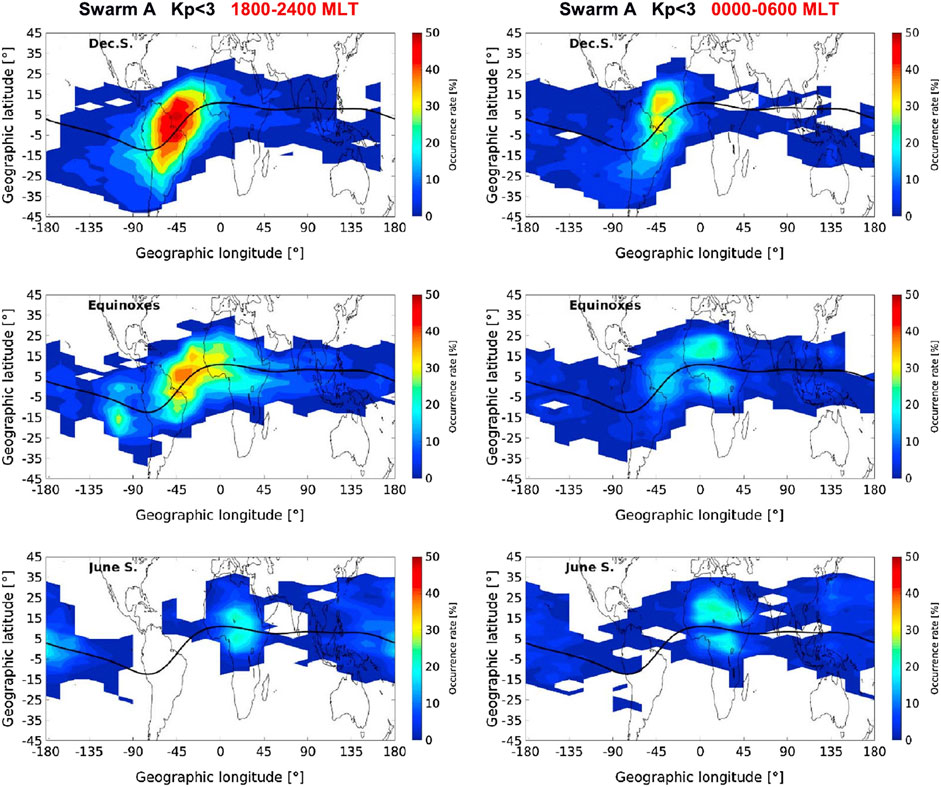
FIGURE 1. Occurrence rate of equatorial plasma depletions as a function of longitude and latitude for (left) post-sunset sector and (right) post-midnight sector (from Wan et al., 2018).

2.3 GOLD

The NASA Global-scale Observations of the Limb and Disk (GOLD) mission has a far ultraviolet imaging spectrograph (∼ 134–162 nm) on the SES-14 communications satellite in geosynchronous orbit at longitude 47.5°W (Eastes et al., 2020). The satellite was launched in January 2018. Measurements made include limb scans, stellar occultations, and images of the sunlit and nightside disk from 6:10 to 00:40 universal time each day. The thermospheric composition ratio O/N₂, temperatures near 160 km, and exospheric temperatures are retrieved from the daytime observations. Molecular oxygen (O₂) densities are measured using stellar occultations. Relevant to equatorial spread F, nighttime emissions from radiative recombination in the ionospheric F region is used to quantify ionospheric density variations in the equatorial ionization anomaly (EIA).

Eastes et al. (2019) reported imaging of the equatorial ionization anomaly that included the solar minimum period October - December 2018. They found the unexpected development of large-scale plasma depletions exhibiting longitudinal structure associated with EPBs which occurred frequently. These observations are unique and provide new information of EPB development on a global scale that has not been achieved before. The results of this study are further discussed in the Global Modeling section.

2.4 ICON

The NASA Ionospheric Connection Explorer (ICON) satellite mission was launched in October 2019 (Immel et al., 2018). It has an orbit 590 × 607 km orbit at 27° inclination so it is well-suited to measure equatorial dynamics. It is instrument package includes 1) the Michelson Interferometer for Global High-resolution Thermospheric Imaging (MIGHTI) which measures the altitude profile of the atmospheric wind and temperature in the Earth’s upper atmosphere, 2) the Ion Velocity Meter (IVM) which measures the in situ ion drift velocity, the ion temperature and the total ion number density, 3) the Extreme Ultraviolet Spectrograph (EUV) which measures the earth’s EUV dayglow, and 4) the Far Ultra Violet Imaging Spectrograph (FUV) which measures the daytime thermospheric composition and altitude profiles of the nighttime ion density. The primary science objectives of ICON are to 1) quantify the relationships between the thermospheric winds, conductances, and electric field in the ionosphere, 2) identify the role of large-scale waves in the neutral atmosphere that propagate from the lower atmosphere to the upper atmosphere, and 3) understand the response of the low-to mid-latitude ionosphere to disturbances in the solar wind.

Although the primary mission did not specify the study of ionospheric irregularities, it is being proposed for an extended mission. ICON has the unique capability of measuring winds in the E and F regions, plasma drifts, and ion densities. The relationship between these quantities can be used to establish the physical underpinnings of the cause and evolution of equatorial ionospheric irregularites and EPBs. For example, Huba et al. (2021) investigated the occurrence of large-scale depletions of O⁺ (but not H⁺) in the post-midnight, topside ionosphere. During the course of this study they also discovered the development of EPBs in the African and Pacific sectors. The IVM detected a series of plasma striations (i.e., bubbles) in the longitude range 240°–330° in the post-midnight local time sector consistent with model results.

3 Theory

The generalized Rayleigh-Taylor instability (GRTI) is considered to be a primary mechanism to initiate equatorial spread F (ESF). The linear theory of the GRTI, using the local approximation, is well-described in Ossakow (1981), Hysell (2000), and Huba (2021). The growth rate is

$\gamma =\frac{1}{L_n}\left[\left(\frac{c{E}_0}{B_0}-V_n\right)+\frac{g}{{\nu }_{in}}\right](1)$

where 1/L_n = ∇n/n is the density gradient scale length, E₀ is the zonal electric field, V_n is the meridional neutral wind, g is gravity, B₀ is the geomagnetic field, and ν_in is the ion-neutral collision frequency. However, Haerendel (1974) recognized that a flux-tube integrated theory of the GRTI was more relevant to ESF because the geomagnetic field lines are essentially equipotentials and the electric field connects the E and F regions. This theory was subsequently elaborated upon by Haerendel et al. (1992) and Sultan (1996). This theory has been applied to develop forecasting methodology for the occurrence of equatorial plasma bubbles (Sultan, 1996; Carter et al., 2014; Wu, 2015). We now highlight two new aspects of the GRTI theory that has emerged over the last several years.

3.1 Meridional winds

The long held conventional wisdom has been that transequatorial neutral winds are a stabilizing influence on the development of EPBs. Maruyama (1988) demonstrated that such a wind enhances the field-line integrated Pedersen conductivity and that this can reduce the growth rate of the generalized Rayleigh-Taylor instability. Zalesak and Huba (1991) extended the analysis of Maruyama (1988) to consider the direct effect of the wind on the development of the instability. They found that, in fact, the instability can be completely stabilized for a sufficiently strong meridional wind. These results were borne out in a 3D simulation study by Krall et al. (2009). However, this result is based on the assumption of a uniform, transequatorial meridional wind.

The observational evidence that meridional winds are a stabilizing influence on ESF is not conclusive Mendillo et al. (1992) performed a limited, 2-day case study using the ALTAIR radar and optical imaging data. They found that ESF was suppressed on the first night but not the next night. They attribute the suppression of ESF on the first night to a north-to-south meridional wind based on a reduction of the northern meridional gradient in 6300 Å airglow. A subsequent study by Mendillo et al. (2001) found ‘no convincing evidence for the wind suppression mechanism.’ A study by Abdu et al. (2006) found magnetic meridional winds negatively influence ESF development by reducing the pre-reversal enhancement electric field and direct suppression of the instability. On the other hand, Devasia et al. (2002) and Jyoti et al. (2004) found that under certain circumstances equatorward neutral winds appeared to be needed for ESF to develop.

The impact of meridional winds on ESF was reexamined by Huba and Krall (2013). They found that transequatorial meridional winds could be stabilizing or destabilizing based on theory and modeling. The key to this result is that they relaxed the assumption of a constant transequatorial meridional wind. They found that a wind profile with a positive gradient as a function of latitude (∂V_m/∂θ ≥ 0) is a stabilizing influence on the generalized Rayleigh-Taylor instability; but a wind profile with a negative gradient (∂V_m/∂θ < 0) is a destabilizing influence. Here, a northward wind is positive and θ increases in the northward direction. It was suggested that meridional wind profiles may account for, in part, the longitudinal and day-to-day variability of ESF.

An example of the impact of different meridional winds on EPB development is shown in Figure 2. Electron density contours are shown as a function of longitude and altitude for equatorward winds (top: case 80eq) and for poleward winds (bottom: case 80po). The equatorward flow case, which has a strong negative meridional wind gradient, has a well-developed plasma bubble that extends to almost 800 km while the poleward flow case, which has a strong positive meridional wind gradient, has only developed a minor density undulation on the bottomside F layer.

FIGURE 2

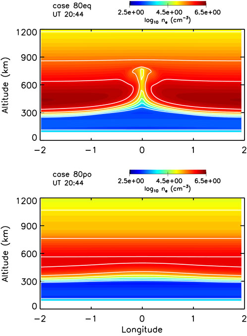
FIGURE 2. Electron density contours as a function of longitude and altitude for a negative wind gradient (top: case 80eq) and a positive wind gradient (bottom: case 80po) (from Huba and Krall, 2013).

3.2 E region drivers

Recently the linear theory of the GRTI was expanded to include inertia, acceleration forces, and E region drivers for both the local approximation and the flux-tube integration method (Huba, 2022). It was found that inertia and acceleration forces do not affect the growth rate of the GRTI for nominal ionospheric conditions, but E region zonal drifts can significantly increase or decrease the growth rate of the GRTI in the equatorial and mid-latitude ionosphere depending on their direction. We will not go through the details of the analysis in Huba (2022) but highlight the essential point. The geometry and drivers considered in the analysis is show in Figure 3. The growth rate of the GRTI is represented as

$\gamma \propto \frac{1}{L_n}\left[\left(\frac{c{E}_{0\varphi }}{B}-V_{np}\right)-\frac{g_p}{{\nu }_{in}}+\frac{{\nu }_{in}}{{\mathrm{\Omega }}_i}\left(\frac{c{E}_{0p}}{B}-V_{n\varphi }\right)\right](2)$

FIGURE 3

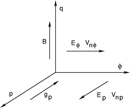
FIGURE 3. Geometry and drivers considered in Huba (2022).

In Eq. 2 the first three terms on the RHS correspond to those shown in Eq. 1. These are the F region drivers that dominate when ν_in ≪Ω_i. On the other hand, when ν_in ≫Ω_i then the last two terms in Eq. 2 can become important. These are the zonal plasma (i.e., cE_0p/B) and neutral wind drifts in the E region and are responsible for equatorial electrojet instabilities (Rogister and D’Angelo, 1970).

An important aspect of this result is the following. An issue with the standard flux-tube integrated theory of the GRTI is that the growth rate of the instability is typically relatively slow: $\sim 8\times 10^{-4}$ s⁻¹ which corresponds to an e-folding time of ∼ 20 min (Sultan, 1996). Based on this it would take over an hour for an EPB to develop (i.e., several e-folding times) which is not consistent with observations. However, if E region drivers are considered then it is possible to increase the growth rate of the GRTI to explain the rapid development of EPBs. This is illustrated in Figure 4 which shows contour plots of the electron density (top), the EF growth rate which only includes F region drivers (middle), and the EE growth rate which includes both the E and F region drivers (bottom) as a function of longitude and altitude (Huba, 2022). The electron density contour shows a weak uplift after sunset (longitude ∼ 120°) but a strong uplift in the pre-dawn sector (longitude ∼ 260°). This latter result has been observed with the C/NOFS satellite during periods of very low F10.7 (Su et al., 2009). The middle panel shows the growth rate of the GRTI for the EF case. It has a maximum during the pre-dawn uplift of ∼ 2.0 × 10⁻³ s⁻¹ which corresponds to a growth time ∼ 8.3 min. The bottom panel shows the growth rate of the GRTI for the EE case. It has a maximum growth rate near the peak uplift of the ionosphere of ∼ 6.2 × 10⁻³ s⁻¹ which corresponds to a growth time ∼ 2.7 min; significantly faster than the EF case.

FIGURE 4

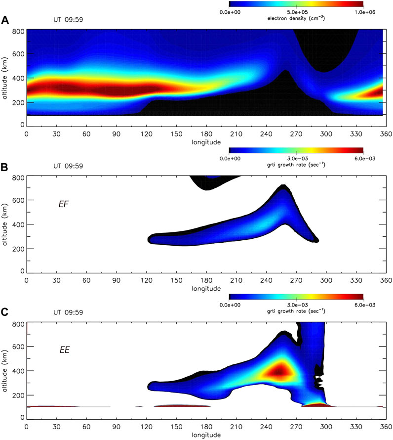
FIGURE 4. Contour plots of the electron density (A), EF growth rate (B), and EE growth rate (C) as a function of longitude and altitude at time ∼ 10:00 UT [from Huba (2022)].

4 Modeling

There have been significant advances in computational modeling of equatorial spread F over the past decade. Reviews of new models have been presented by Yokoyama (2017) and Huba (2021). The original ESF bubble models were two-dimensional in space (i.e., in the plane orthogonal to the geomagnetic field) and considered an idealized ionosphere background (Zalesak and Ossakow, 1980; Zalesak et al., 1982). Newer ESF bubble models have been developed that are three-dimensional in space and include transport along the magnetic field for realistic background ionosphere conditions (Huba et al., 2008; Retterer, 2010a; Retterer, 2010b; Yokoyama et al., 2014; Yokoyama et al., 2015). These models assume equipotential field lines, i.e., the electrostatic potential does not vary along the magnetic field. Additionally, these models only considered a narrow wedge of the ionosphere, i.e., a limited range of longitudes, typically a few degrees. Three-dimensional models have also been developed that relax the equipotential field line assumption and solve a three-dimensional potential equation so the potential can vary along the magnetic field (Kherani et al., 2005; Aveiro and Hysell, 2010; Aveiro and Hysell, 2012; Aveiro and Huba, 2013). And lastly, data-driven numerical ESF models have been developed (Hysell et al., 2014a; Hysell et al., 2014b). We highlight two new model developments that indicate a significant path forward to understanding and forecasting equatorial spread F.

4.1 Data driven modeling

Recently, the onset and evolution of ESF bubbles has been studied using a data-driven methodology (Hysell et al., 2014a; Hysell et al., 2014b; Hysell et al., 2014c; Hysell et al., 2015). The 3D space/3D potential model developed by Aveiro and Hysell (2012) is initialized using ionospheric and neutral wind data at Jicamarca. The model is then run to determine whether or not ESF bubbles are generated for these conditions and the results compared to radar backscatter data at Jicamarca.

In Hysell et al. (2014a), the Jicamarca Radio Observatory measured the ionosphere electron density, vector drift velocity, the neutral winds, and coherent radar backscatter from plasma irregularities during a campaign running from 12 to 18 April 2013. The 3D model was initialized with a combination of data and empirical models was used. The electron density was specified using the Parameterized Ionosphere Model (PIM) (Daniell et al., 1995) where it was ‘nudged’ to match the Jicamarca radar measured value of the electron density. The International Reference Ionosphere (IRI 2007) (Bilitza and Reinisch, 2008) was used to determine the plasma composition. An imposed background zonal electric field and neutral wind profile, both varying in time and longitude, are used. The zonal electric field is obtained from height-averaged Jicamarca plasma drift measurements, while the neutral wind profile is determined from fitting FPI measurements to the empirical wind model HWM07 (Drob et al., 2008). A similar study was carried out (Hysell et al., 2014b) focused on the 2013 Autumnal equinox.

The model predictions of ESF bubble development were in good agreement with the observations. In Hysell et al. (2014a) it was noted that the bottom-type layers observed on a day of moderate activity (weak plumes) were stronger than a day with low activity (no plumes) conditions, contrary to the simulation results. It was suggested that this was caused by an inadequate specification of the neutral wind, the most important variable for driving collisional shear instability. In Hysell et al. (2014b) the modeling results were also in good agreement with observations. The simulations failed to reproduce two significant events. Hysell et al. (2015) performed yet another study focusing on April and December of 2014. One notable improvement in this study is that it used the upgraded horizontal wind model HWM14 (Drob et al., 2015). The simulations were able to determine whether or not large plasma ESF bubbles form and penetrate through to the topside. Significantly, the simulations did not produce any “false alarms.”

Recently, Hysell et al. (2022) reported results from a data driven simulation that used the global atmosphere/ionosphere/plasmasphere GCM (WAM-IPE) to forecast irregularities associated with equatorial spread F (ESF) the post-sunset sector. A regional simulation was first performed using ionosphere parameters derived from Jicamarca Radio Observatory observations and empirical models, similar to earlier data driven simulations. The irregularities produced were found to be similar to those observed. Subsequently, several simulations were performed using state parameters from WAM-IPE. They found that in one of five cases studied, the forecast failed to accurately predict ESF irregularities due to the late reversal of the zonal thermospheric winds. More significantly, in four of five cases there were major differences between the observed and predicted prereversal enhancement (PRE) of the background electric field. This resulted in a poor forecast accuracy for EPB development.

Based on this work one could argue that the problem of large scale equatorial plasma bubble development has been solved. The fundamental plasma equations being solved in the computational model appear adequate to describe the phenomenon; the only caveat is that the background ionosphere and thermosphere conditions need to be known accurately. Thus, the technique provides a ‘nowcast’ to EPB development using observational measurements of the plasma and neutral states. To provide a forecast of EPB development would require an accurate forecast model of the ionosphere/thermosphere system.

4.2 Global modeling

As indicated in the previous section, data-driven models of ESF appear to be a very promising tool in forecasting bubble development. However, two shortcomings of many 3D ESF models are that they are limited to a narrow wedge (e.g., $\sim 4°$) of the post-sunset ionosphere, and they do not include a self-consistent neutral wind driven dynamo electric field. To overcome these shortcomings, a self-consistent global ionosphere/thermosphere model is required with grid scales sufficiently small (e.g., ≲ 10 s km) to capture the onset and evolution of ESF plasma bubbles.

Huba and Joyce (2010) made a substantial step forward by adapting the global ionosphere model SAMI3 to include a high-resolution sub-grid that allows for the development of ESF plasma bubbles. We mention Eccles (1999) performed a similar analysis. However, a simplistic, 2D flux-tube integrated plasma model was used that only included O⁺ and a single molecular mixture of NO⁺ and ${\mathrm{O}}_2^{+}$ Huba and Joyce (2010) modified the global ionosphere model SAMI3 to include a high resolution longitudinal grid in the pre-to post-sunset sector (1630 MLT - 2230 MLT) to capture the evolution of equatorial plasma bubbles. The neutral composition and temperature were specified using NRLMSISE00 (Picone et al., 2002), and the neutral wind is specified using HWM93 (Hedin et al., 1991). In order to initiate the development of EPBs, a series of Gaussian-like perturbations in the ion density were imposed at t = 0 in the pre- and post-sunset sectors.

An example of the results from Huba and Joyce (2010) is shown in Figure 5. Electron density contours as a function of magnetic local time (MLT) and altitude (km) at 0° longitude are shown. If Figure 5A a the ionosphere builds up after sunrise (0600 MLT) and reaches a maximum electron density in mid-afternoon (∼ 1500 MLT). Subsequently the ionosphere is lifted to higher altitudes because of the pre-reversal enhancement (PRE) of the eastward electric field (peaking at ∼ 1800 MLT). Finally, the ionosphere descends and weakens throughout the nighttime hours (i.e., 2100 MLT - 0600 MLT). This is nominally the standard behavior of the ionosphere. The imposed perturbations on the electron density are weakly evident in the contours around 1800 MLT. At later times, large scale plasma bubbles develop (between ∼ 1940–2100 MLT) as shown in Figure 5B. These bubbles were triggered by the imposed perturbations at the outset of the simulation except for the last bubble at time ∼ 2000 MLT). This bubble was initiated by downward flows associated with the plasma bubble preceding it.

FIGURE 5

FIGURE 5. Electron density contours as a function of magnetic local time (MLT) and altitude (km) at 0° longitude are shown at times (A) 00:10 UT and (B) 02:20 UT (from Huba and Joyce, 2010).

There are several shortcomings of the model developed by Huba and Joyce (2010) in the quest to accurately model the onset and development of EPBs. First, it used a centered-dipole geomagnetic field which limits the code’s ability to capture seasonal and longitudinal variations of EPB development. Second, it used the donor cell method for cross-field transport which is a diffusive transport algorithm and inhibits the development of complex EPB structures. And lastly, it used an artificial ion perturbation seed to intitiate EPBs as opposed to a more realistic seeding mechanism such as gravity waves.

These shortcomings were overcome in a recent study by Huba and Liu (2020). This work demonstrated that large-scale equatorial spread F (ESF) plasma bubbles could develop in the post-sunset ionosphere using a global ionosphere/thermosphere model. The coupled model comprises the ionospheric code SAMI3 (based on SAMI3 (Huba et al., 2000)) and the atmosphere/thermosphere code WACCM-X (Liu et al., 2018). The model is one-way coupled in that WACCM-X provides the thermosphere inputs to SAMI3 (i.e., neutral densities, termperature, and winds) by SAMI3 does not supply any ionospheric inputs into WACCM-X. In addition to self-consistently modeling the thermosphere, WACCM-X also includes gravity waves (via parameterization) which provide natural seeds to trigger EPBs. Lastly, the SAMI3 model used implemented a 4th order flux-corrected transport scheme for E × B transport perpendicular to the magnetic field. The partial donor cell method (Hain, 1987; Huba, 2003) was used which reduces numerical diffusion and allows steeper density gradients to develop. Two cases are modeled for different seasons and geophysical conditions: the March case (low solar activity: F10.7 = 70) and the July case (high solar activity: F10.7 = 170). We find that equatorial plasma bubbles formed and penetrated into the topside F layer for the March case but not the July case; consistent with ESF climatology [ ].

In Figure 6 we compare 135.6 nm emissions from the simulation for the March case at 23:59 UT (left and middle panels) to GOLD emission observations (right panel) from geosynchronous orbit (Eastes et al., 2019). The GOLD results are for October 2018 which corresponds to equinox conditions at solar minimum, similar to the conditions of the simulation. An interesting result of this work is shown in Figure 6. Here, is a comparison of 135.6 nm emissions from the simulation for the March case at 23:59 UT (left and middle panels) to GOLD emission observations (right panel) from geosynchronous orbit (Eastes et al., 2019). The GOLD results are for October 2018 which corresponds to equinox conditions at solar minimum, similar to the conditions of the simulation. The center panel is on the same color scale as the GOLD data (maximum of 40 Rayleighs); it shows that the intensity of the 135.6 nm emissions from the model is less than the data. The left panel reduces the color scale maximum to 12 Rayleighs in order to highlight the structure in the model results; it shows a remarkable similarity to the data. The model results capture the extended ionization arcs from the post-sunset period (eastern South America) to midnight (western Africa) observed in the data. Moreover, regular plasma striations (bubbles) are also observed in the model as in the data on similar scale lengths.

FIGURE 6

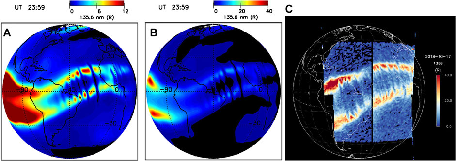
FIGURE 6. Comparison of 135.6 nm emissions from the simulation for the March case (A, B) and GOLD emission data (C) observed from geosynchronous orbit (Eastes et al., 2019).

5 Where do we stand?

As noted in the Introduction, Woodman (2009) addressed the problem of ESF and the status of its ‘solution’ over a decade ago. In his final section, also entitled ‘Where do we stand?,’ he notes that progress has been very slow in coming to grips with ESF. Although the fundamenatal theories of the instabilities responsible for ESF seemed to be in hand, and progress had been made in the computational modeling of a number of instabilities, there remains an inability to understand it is day-to-day variability. Woodman (2009) argued this was primarily because of a lack of neutral wind data, a dominant factor in controlling ESF.

The current situation of understanding ESF has improved considerably over the past decade. A wealth of new observational data from in situ satellite measurements has been acquired. Data continues to be obtained from ground-based radar systems, as well as GPS TEC data, but we have focused on satellite data because it provides global coverage over a solar cycle and establishes a more complete picture of equatorial density irregularities as a function of season, solar activity, and longitude. Moreover, a global perspective of equatorial plasma bubbles (EPBs) has emerged from the NASA GOLD mission, and the NASA ICON mission is making unprecedented measurements of the neutral wind with the MIGHTI instrument in conjunction with in situ measurements of ion densities, velocities, and temperature with the IVM instrument. New theoretical analyses (Huba and Krall, 2013; Huba, 2022) have shed new light on the role of neutral winds and electric fields on the development of ESF through the generalized Rayleigh-Taylor instability. Perhaps more significantly there has been major improvements in the modeling capability of ESF (Yokoyama, 2017; Huba and Liu, 2020).

But there still remains a number of issues to be resolved. As noted in the Introduction, the spatial scales of electron density irregularities in the equatorial ionosphere range from 100 s km to 10 s cm. One of the unsolved problems noted in Woodman (2009) is understanding the physical mechanisms to generate turbulence over this range and the spectral behavior of this turbulence. Haerendel (1974) proposed a hierarchy of instabilities operating at different length scales to explain this range of turbulence. Although conceptually this remains relevant, there is still no unified theory/model to capture the physics of this system. One problem is modeling the irregularities from the global scale to 100 s m (the Fresnel scale for L-band signals is 300–400 m; these scale lengths are responsible for signal scintillation). Yokoyama (2017) has presented the highest resolution simulation result to date with grid sizes ∼ 300 m. Spectral analysis of the results are shown in Figure 7 which are remarkable but higher resolution is still needed.

FIGURE 7

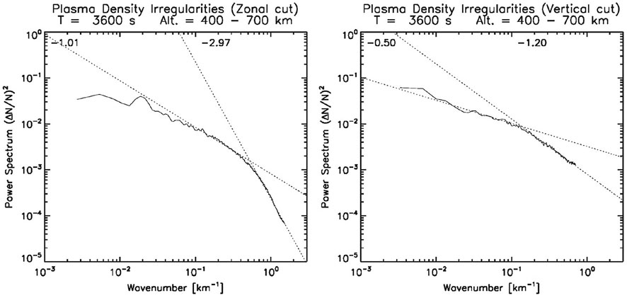
FIGURE 7. Power spectral density plots of irregularities from a high-resolution computational model (from Yokoyama, 2017).

The more challenging issue is addressing turbulent scales below 100 m in a unified manner because kinetic physics becomes important (e.g., finite Larmor radius effects, demagnetization of the ions). For example, radar backscatter measurements detect irregularities with scale lengths of 36 cm, 1 m, and 3 m (Woodman, 2009). Huba et al. (1978) demonstrated that the ion cyclotron and lower-hybrid-drift instabilities are viable candidates to explain the 1 m and 3 m irregularities but not the 3 m irregularities. Costa and Kelley (1978) proposed the universal drift instability as a mechanism to explain the 3 m irregularities but Huba and Ossakow (1979) argued against this because the instability would be damped by ion viscosity. To date there is still no explanation for the 3 m irregularities. Perhaps the more likely scenario is that these waves are generated via a nonlinear cascade from longer wavelength turbulence (or perhaps from shorter wavelength turbulence). A particle-in-cell code or hybrid code that included collisions would be needed to address this problem more fully.

Another area that has not been fully explored is the development of equatorial plasma bubbles during geomagnetic storms (Abdu, 2012). In this situation, stormtime penetration electric fields and disturbance dynamo fields impact the low-to mid-latitude ionosphere and can excite (or possibly suppress) EPBs. These stormtime fields have not been included in any global simulation studies yet. A path forward to address this issue would be to couple a whole atmosphere model (e.g., WACCM-X) to a ionosphere/ring current model (e.g., SAMI3/RCM (Huba and Sazykin, 2014)).

From a forecasting point of view, it has been noted that perhaps the most important parameter that needs to be known is the neutral wind (Hysell et al. (2022)). The zonal wind predominantly determines the ionospheric electric field, and in particular the PRE which can play a crucial role is the onset of ESF. Additionally, the transequatorial meridional neutral wind can act to stabilize or destabilize the GRTI (Huba and Krall, 2013). To this end high-resolution, whole atmosphere models have been developed and are being improved to forecast the thermospheric winds (e.g., WACCM-X (Liu et al., 2018 and HIAMCM (Becker et al., 2022). Moreover, the NASA ICON mission has provided, and hopefully will continue to provide, thermospheric winds on a global scale that can be used in equatorial dynamics studies.

Lastly, the preponderance of ESF occurrence is during solar maximum condtions in the American/Atlantic sector and is related to strong PRE upward drifts. The EPBs associated with these occurrences can often persist after midnight and are referred to as ‘fossil bubbles.’ However, there are also observations of ESF occurring in the post-midnight sector during solar minimum conditions for the June solstice in the absence of post-sunset EPBs (Heelis et al., 2010; Li et al., 2011; Zhan et al., 2018). This area of ESF research has not been fully explored with modeling and deserves attention.

Data availability statement

The original contributions presented in the study are included in the article/supplementary material, further inquiries can be directed to the corresponding author.

Author contributions

The author confirms being the sole contributor of this work and has approved it for publication.

Funding

This research has been funded by NASA grant 80NSSC21K1305, the NASA ICON Explorers Program through contracts NNG12FA45C and NNG12FA42I, and NSF grant AGS-1931415.

Conflict of interest

Author JH was employed by Syntek Technologies, Inc., Fairfax, VA, United States.

Publisher’s note

All claims expressed in this article are solely those of the authors and do not necessarily represent those of their affiliated organizations, or those of the publisher, the editors and the reviewers. Any product that may be evaluated in this article, or claim that may be made by its manufacturer, is not guaranteed or endorsed by the publisher.

References

Abdu, M. A., Iyer, K. N., de Medeiros, R. T., Batista, I. S., and Sobral, J. H. A. (2006). Thermospheric meridional wind control of equatorial spread F and evening prereversal electric field. Geophys. Res. Lett. 33, L07106. doi:10.1029/2005GL024835

CrossRef Full Text | Google Scholar

Abdu, M. A. (2012). Equatorial spread F/plasma bubble irregularities under storm time disturbance electric fields. J. Atmos. Sol. Terr. Phys. 75, 44–56. doi:10.1016/j.jastp.2011.04.024

CrossRef Full Text | Google Scholar

Aveiro, H. C., and Huba, J. D. (2013). Equatorial spread F studies using SAMI3 with two-dimensional and three-dimensional electrostatics. Ann. Geophys. 31, 2157–2162. doi:10.5194/angeo-31-2157-2013

CrossRef Full Text | Google Scholar

Aveiro, H. C., and Hysell, D. L. (2010). Forecast assessment of topside spread F at Jicamarca. J. Geophys. Res. 115, A12331. doi:10.1029/2010JA015990

CrossRef Full Text | Google Scholar

Aveiro, H. C., and Hysell, D. L. (2012). Three-dimensional numerical simulation of equatorial F region plasma irregularities with bottomside shear flow. J. Geophys. Res. 115, A11321. doi:10.1029/2010JA015602

CrossRef Full Text | Google Scholar

Becker, E., Vadas, S. L., Bossert, K., Harvey, V. L., Zulicke, C., and Hoffmann, L. (2022). A High-resolution whole-atmosphere model with resolved gravity waves and specified large-scale dynamics in the troposphere and stratosphere. J. Geophys. Res. Atmos. 127, e2021JD035018. doi:10.1029/2021JD035018

CrossRef Full Text | Google Scholar

Bilitza, D., and Reinisch, B. W. (2008). International Reference ionosphere 2007: Improvements and new parameters. Adv. Space Res. 42, 599–609. doi:10.1016/j.asr.2007.07.048

CrossRef Full Text | Google Scholar

Booker, H. G., and Wells, H. G. (1938). Scattering of radio waves by the F-region of the ionosphere. J. Geophys. Res. 43, 249. doi:10.1029/te043i003p00249

CrossRef Full Text | Google Scholar

Burke, W. J., de La Beaujardière, O., Gentile, L. C., Hunton, D. E., Pfaff, R. F., Roddy, P. A., et al. (2009). C/NOFS observations of plasma density and electric field irregularities at post-midnight local times. Geophys. Res. Lett. 36, L00C09. doi:10.1029/2009GL038879

CrossRef Full Text | Google Scholar

Carter, B. A., Retterer, J. M., Yizengaw, E., Groves, K., Caton, R., McNamara, L., et al. (2014). Geomagnetic control of equatorial plasma bubble activity modeled by the TIEGCM with Kp. Geophys. Res. Lett. 41, 5331–5339. doi:10.1002/2014GL060953

CrossRef Full Text | Google Scholar

Costa, E., and Kelley, M. C. (1978). Linear theory for the collisionless drift wave instability with wavelengths near the ion gyroradius. J. Geophys. Res. 83, 4365. doi:10.1029/ja083ia09p04365

CrossRef Full Text | Google Scholar

Daniell, R. E., Brown, L. D., Anderson, D. N., Fox, M. W., Doherty, P. H., Decker, D. T., et al. (1995). Parameterized ionospheric model: A global ionospheric parameterization based on first principles models. Radio Sci. 30, 1499–1510. doi:10.1029/95rs01826

CrossRef Full Text | Google Scholar

de La Beaujardiere, O. (2004). C/NOFS: a mission to forecast scintillations. J. Atmos. Sol. Terr. Phys. 66, 1573–1591. doi:10.1016/j.jastp.2004.07.030

CrossRef Full Text | Google Scholar

Devasia, C. V., Jyoti, N., Viswanathan, K. S., et al. (2002). On the plausible leakage of thermospheric meridional winds with equatorial spread F. J. Atmos. Sol. Terr. Phys. 64 (1), 1–12. doi:10.1016/S1364-6826(01)00089-X

CrossRef Full Text | Google Scholar

Drob, D. P., Emmert, J. T., Crowley, G., Picone, J. M., Shepherd, G. G., Skinner, W., et al. (2008). An empirical model of the earth’s horizontal wind fields: HWM07. J. Geophys. Res. 113, A12304. doi:10.1029/2008JA013668

CrossRef Full Text | Google Scholar

Drob, D. P., Emmert, J. T., Meriwether, J. W., Makela, J. J., Doornbos, E., Conde, M., et al. (2015). An update to the Horizontal Wind Model (HWM): The quiet time thermosphere. Earth Space Sci. 2, 301–319. doi:10.1002/2014EA000089

CrossRef Full Text | Google Scholar

Eastes, R. W., Solomon, S. C., Daniell, R. E., Anderson, D. N., Burns, A. G., England, S. L., et al. (2019). Global-scale observations of the equatorial ionization anomaly. Geophys. Res. Lett. 46, 9318–9326. doi:10.1029/2019GL084199

CrossRef Full Text | Google Scholar

Eastes, R. W., McClintock, W. E., Burns, A. G., Anderson, D. N., Andersson, L., Aryal, S., et al. (2020). Initial observations by the GOLD mission. JGR. Space Phys. 125, e2020JA027823. doi:10.1029/2020JA027823

CrossRef Full Text | Google Scholar

Eccles, J. V. (1999). “Geophysically realistic models of ESF plasma plumes,” in Proceeding Ionospheric Effects Symposium. Editor J.M. Goodman, 545.

Google Scholar

Haerendel, G., Eccles, J. V., and Çakir, S. (1992). Theory for modeling the equatorial evening ionosphere and the origin of the shear in the horizontal plasma flow. J. Geophys. Res. 97, 1209. doi:10.1029/91ja02226

CrossRef Full Text | Google Scholar

Haerendel, G. (1974). Theory of equatorial spread F, preprint. Munich, Germany: Max Planck Institute for Extraterrestrial Physics.

Google Scholar

Hain, K. (1987). The partial donor cell method. J. Comput. Phys. 73, 131–147. doi:10.1016/0021-9991(87)90110-0

CrossRef Full Text | Google Scholar

Hedin, A. E., Biondi, M. A., Burnside, R. G., Hernandez, G., Johnson, R. M., Killeen, T. L., et al. (1991). Revised global model of thermosphere winds using satellite and ground-based observations. J. Geophys. Res. 96, 7657. doi:10.1029/91ja00251

CrossRef Full Text | Google Scholar

Heelis, R. A., Stoneback, R., Earle, G. D., Haaser, R. A., and Abdu, M. A. (2010). Medium-scale equatorial plasma irregularities observed by coupled ion-neutral dynamics investigation sensors aboard the communication navigation outage forecast system in a prolonged solar minimum. J. Geophys. Res. 115, A10321. doi:10.1029/2010JA015596

CrossRef Full Text | Google Scholar

Huang, C.-S., and Hairston, M. R. (2015). The postsunset vertical plasma drift and its effects on the generation of equatorial plasma bubbles observed by the C/NOFS satellite. J. Geophys. Res. Space Phys. 120, 2263–2275. doi:10.1002/2014JA020735

CrossRef Full Text | Google Scholar

Huang, C.-S., de La Beaujardiere, O., Roddy, P. A., Hunton, D. E., Ballenthin, J. O., and Hairston, M. R. (2012). Generation and characteristics of equatorial plasma bubbles detected by the C/NOFS satellite near the sunset terminator. J. Geophys. Res. 117, A11313. doi:10.1029/2012JA018163

CrossRef Full Text | Google Scholar

Huang, C.-S., de La Beaujardiere, O., Roddy, P. A., Hunton, D. E., Liu, J. Y., and Chen, S. P. (2014). Occurrence probability and amplitude of equatorial ionospheric irregularities associated with plasma bubbles during low and moderate solar activities (2008–2012). J. Geophys. Res. Space Phys. 119, 1186–1199. doi:10.1002/2013JA019212

CrossRef Full Text | Google Scholar

Huang, C.-S. (2017). The characteristics and generation mechanism of small-amplitude and large-amplitude ESF irregularities observed by the C/NOFS satellite. J. Geophys. Res. Space Phys. 122, 8959–8973. doi:10.1002/2017JA024041

CrossRef Full Text | Google Scholar

Huba, J. D., and Joyce, G. (2010). Global modeling of equatorial plasma bubbles. Geophys. Res. Lett. 37, L17104. doi:10.1029/2010GL044281

CrossRef Full Text | Google Scholar

Huba, J. D., and Krall, J. (2013). Impact of meridional winds on equatorial spread F: Revisited. Geophys. Res. Lett. 40, 1268–1272. doi:10.1002/grl.50292

CrossRef Full Text | Google Scholar

Huba, J. D., and Liu, H.-L. (2020). Global modeling of equatorial spread F with SAMI3/WACCM-X. Geophys. Res. Lett. 47, e2020GL088258. doi:10.1029/2020gl088258

CrossRef Full Text | Google Scholar

Huba, J. D., and Ossakow, S. L. (1979). On the generation of 3 meter irregularities during equatorial spread F by low frequency drift waves. J. Geophys. Res. 84, 6697. doi:10.1029/ja084ia11p06697

CrossRef Full Text | Google Scholar

Huba, J. D., and Sazykin, S. (2014). Storm time ionosphere and plasmasphere structuring: SAMI3-RCM simulation of the 31 March 2001 geomagnetic storm. Geophys. Res. Lett. 41, 8208–8214. doi:10.1002/2014gl062110

CrossRef Full Text | Google Scholar

Huba, J. D., Chaturvedi, P. K., Ossakow, S. L., and ToMe, D. M. (1978). High frequency drift waves with wavelengths below the iongyroradius in equatorial spread F. Geophys. Res. Lett. 5, 695–698. doi:10.1029/gl005i008p00695

CrossRef Full Text | Google Scholar

Huba, J. D., Joyce, G., and Fedder, J. A. (2000). Sami2 is another model of the ionosphere (SAMI2): A new low-latitude ionosphere model. J. Geophys. Res. 105, 23035–23053. doi:10.1029/2000ja000035

CrossRef Full Text | Google Scholar

Huba, J. D., Joyce, G., and Krall, J. (2008). Three-dimensional equatorial spread F modeling. Geophys. Res. Lett. 35, L10102. doi:10.1029/2008GL033509

CrossRef Full Text | Google Scholar

Huba, J. D., Heelis, R., and Maute, A. (2021). Large-scale O⁺ depletions observed by ICON in the post-midnight topside ionosphere: Data/model comparison. Geophys. Res. Lett. 48, e2020GL0920061. doi:10.1029/2020gl092061

CrossRef Full Text | Google Scholar

Huba, J. D. (2003). “A tutorial on Hall magnetohydrodynamics,” in Space simulations. Editors M. Scholer, C. T. Dum, and J. Büchner (New York: Springer), 170.

Google Scholar

Huba, J. D. (2021). “Theory and modeling of equatorial spread F,” in Ionospheric dynamics and applications, geophysical monograph 260. Editors C. Huang, and G. Lu (American Geophysical Union, Wiley). doi:10.1002/9781119815617.ch10

CrossRef Full Text | Google Scholar

Huba, J. D. (2022). Generalized Rayleigh-Taylor instability: Ion inertia, acceleration forces, and E region drivers. JGR. Space Phys. 127, e2022JA030474. doi:10.1029/2022JA030474

CrossRef Full Text | Google Scholar

Hysell, D. L., Jafari, R., Milla, M. A., and Meriwether, J. W. (2014a). Data-driven numerical simulations of equatorial spread F in the Peruvian sector. J. Geophys. Res. Space Phys. 119, 3815–3827. doi:10.1002/2014JA019889

CrossRef Full Text | Google Scholar

Hysell, D. L., Jafari, R., Milla, M. A., and Meriwether, J. W. (2014b). Data-driven numerical simulations of equatorial spread F in the Peruvian sector: 2. Autumnal equinox. J. Geophys. Res. Space Phys. 119, 6981–6993. doi:10.1002/2014JA020345

CrossRef Full Text | Google Scholar

Hysell, D. L., Jafari, R., Fritts, D. C., and Laughman, B. (2014c). Gravity wave effects on postsunset equatorial F region stability. J. Geophys. Res. Space Phys. 119, 5847–5860. doi:10.1002/2014JA019990

CrossRef Full Text | Google Scholar

Hysell, D. L., Milla, M. A., Condori, L., and Vierinen, J. (2015). Data-driven numerical simulations of equatorial spread F in the Peruvian sector 3: Solstice. J. Geophys. Res. Space Phys. 120, 10,809–10,822. doi:10.1002/2015JA021877

CrossRef Full Text | Google Scholar

Hysell, D. L., Fang, T. W., and Fuller-Rowell, T. J. (2022). Modeling equatorial F-region ionospheric instability using a regional ionospheric irregularity model and WAM-IPE. J. Geophys. Res. Space Phys. 127, e2022JA030513. doi:10.1029/2022JA030513

CrossRef Full Text | Google Scholar

Hysell, D. L. (2000). An overview and synthesis of plasma irregularities in equatorial spread F. J. Atmos. Sol. Terr. Phys. 62, 1037–1056. doi:10.1016/s1364-6826(00)00095-x

CrossRef Full Text | Google Scholar

Immel, T. J., England, S. L., Mende, S. B., Heelis, R. A., Englert, C. R., Edelstein, J., et al. (2018). The ionospheric connection explorer mission: Mission goals and design. Space Sci. Rev. 214, 13. doi:10.1007/s11214-017-0449-2

PubMed Abstract | CrossRef Full Text | Google Scholar

Jyoti, N., Devasia, C. V., Sridharan, R., and Tiwari, D. (2004). Threshold height (h’F)_c for the meridional wind to play a deterministic role in the bottom side equatorial spread F and its dependence on solar activity. Geophys. Res. Lett. 31, L12809. doi:10.1029/2004GL019455

CrossRef Full Text | Google Scholar

Kherani, E. A., Mascarenhas, M., Sobral, J. H. A., de Paula, E. R., and Bertoni, F. C. (2005). A three-dimensional simulation of collisional-interchange-instability in the equatorial-low-latitude ionosphere. Space Sci. Rev. 121, 253–269. doi:10.1007/s11214-006-6158-x

CrossRef Full Text | Google Scholar

Krall, J., Huba, J. D., Joyce, G., and Zalesak, S. T. (2009). Three-dimensional simulation of equatorial spread F with meridional wind effects. Ann. Geophys. 27, 1821–1830. doi:10.5194/angeo-27-1821-2009

CrossRef Full Text | Google Scholar

Li, G., Ning, B., Abdu, M. A., Yue, X., Liu, L., Wan, W., et al. (2011). On the occurrence of postmidnight equatorial F region irregularities during the June solstice. J. Geophys. Res. 116, A04318. doi:10.1029/2010JA016056

CrossRef Full Text | Google Scholar

Liu, H.-L., Bardeen, C. G., Foster, B. T., Lauritzen, P., Liu, J., Lu, G., et al. (2018). Development and validation of the whole atmosphere community climate model with thermosphere and ionosphere extension (WACCM-X 2.0). J. Adv. Model. Earth Syst. 10, 381–402. doi:10.1002/2017ms001232

CrossRef Full Text | Google Scholar

Maruyama, T. (1988). A diagnostic model for equatorial spread F, 1, Model description and application to electric field and neutral wind effects. J. Geophys. Res. 93 (14), 14611. doi:10.1029/ja093ia12p14611

CrossRef Full Text | Google Scholar

Mendillo, M., Baumgardner, J., Pi, X., Sultan, P., and Tsunoda, R. (1992). Onset conditions for equatorial spread F. J. Geophys. Res. 97 (13), 13865. doi:10.1029/92ja00647

CrossRef Full Text | Google Scholar

Mendillo, M., Meriwether, J., and Biondi, M. (2001). Testing the thermospheric neutral wind suppression mechanism for day-to-day variability of equatorial spread F. J. Geophys. Res. 106, 3655–3663. doi:10.1029/2000ja000148

CrossRef Full Text | Google Scholar

Ossakow, S. L. (1981). Spread F theories - a review. J. Atmos. Terr. Phys. 43, 437–452. doi:10.1016/0021-9169(81)90107-0

CrossRef Full Text | Google Scholar

Picone, J. M., Hedin, A. E., Drob, D. P., and Aikin, A. C. (2002). NRLMSISE-00 empirical model of the atmosphere: Statistical comparisons and scientific issues. J. Geophys. Res. 107, SIA 15-21–SIA 15-16. doi:10.1029/2002JA009430

CrossRef Full Text | Google Scholar

Retterer, J. M. (2010a). Forecasting low-latitude radio scintillation with 3-D ionospheric plume models: 1. Plume model. J. Geophys. Res. 115, A03306. doi:10.1029/2008JA013839

CrossRef Full Text | Google Scholar

Retterer, J. M. (2010b). Forecasting low-latitude radio scintillation with 3-D ionospheric plume models: 2. Scintillation calculation. J. Geophys. Res. 115, A03307. doi:10.1029/2008JA013840

CrossRef Full Text | Google Scholar

Rogister, A., and D’Angelo, N. (1970). Type II irregularities in the equatorial electrojet. J. Geophys. Res. 75, 3879–3887. doi:10.1029/ja075i019p03879

CrossRef Full Text | Google Scholar

Su, Y.-J., Retterer, J. M., de La Beaujardière, O., Burke, W. J., Roddy, P. A., Pfaff, R. F., et al. (2009). Assimilative modeling of equatorial plasma depletions observed by C/NOFS. Geophys. Res. Lett. 36, L00C02. doi:10.1029/2009GL038946

CrossRef Full Text | Google Scholar

Sultan, P. J. (1996). Linear theory and modeling of the Rayleigh-Taylor instability leading to the occurrence of equatorial spread F. J. Geophys. Res. 101 (26), 26875–26891. doi:10.1029/96ja00682

CrossRef Full Text | Google Scholar

Tsunoda, R. T. (2021). “Observations of equatorial spread F: A working hypothesis,” in Ionospheric dynamics and applications, geophysical monograph 260. Editors C. Huang, and G. Lu (American Geophysical Union, Wiley). doi:10.1002/9781119815617.ch11

CrossRef Full Text | Google Scholar

Wan, X., Xiong, C., Rodriguez-Zuluaga, J., Kervalishvili, G. N., Stolle, C., and Wang, H. (2018). Climatology of the occurrence rate and amplitudes of local time dis- tinguished equatorial plasma depletions observed by Swarm satellite. J. Geophys. Res. Space Phys. 123, 3014–3026. doi:10.1002/2017JA025072

CrossRef Full Text | Google Scholar

Woodman, R. F. (2009). Spread F - an old equatorial aeronomy problem finally resolved? Ann. Geophys. 27, 1915–1934. doi:10.5194/angeo-27-1915-2009

CrossRef Full Text | Google Scholar

Wu, Q. (2015). Longitudinal and seasonal variation of the equatorial flux tube integrated Rayleigh-Taylor instability growth rate. J. Geophys. Res. Space Phys. 120, 7952–7957. doi:10.1002/2015JA021553

CrossRef Full Text | Google Scholar

Xiong, C., Stolle, C., Lühr, H., Park, J., Fejer, B. G., and Kervalishivili, G. (2016). Scale analysis of equatorial plasma irregularities derived from Swarm constellation. Earth Planets Space 68, 121. doi:10.1186/s40623-016-0502-5

CrossRef Full Text | Google Scholar

Yokoyama, T., Shinagawa, H., and Jin, H. (2014). Nonlinear growth, bifurcation, and pinching of equatorial plasma bubble simulated by three-dimensional high-resolution bubble model. J. Geophys. Res. Space Phys. 119, 10474. doi:10.1002/2014JA020708

CrossRef Full Text | Google Scholar

Yokoyama, T., Shinagawa, H., and Jin, H. (2015). Nonlinear growth, bifurcation and pinching of equatorial plasma bubble simulated by three-dimensional high-resolution bubble model. J. Geophys. Res. Space Phys. 119 (10), 474. doi:10.1002/2014JA020708

CrossRef Full Text | Google Scholar

Yokoyama, T. (2017). A review on the numerical simulation of equatorial plasma bubbles toward scintillation evaluation and forecasting. Prog. Earth Planet. Sci. 4, 37. doi:10.1186/s40645-017-0153-6

CrossRef Full Text | Google Scholar

Zakharenkova, I., Astafyeva, E., and Cherniak, I. (2016). GPS and in situ Swarm observations of the equatorial plasma density irregularities in the topside ionosphere. Earth Planets Space 68, 120. doi:10.1186/s40623-016-0490-5

CrossRef Full Text | Google Scholar

Zalesak, S. T., and Huba, J. D. (1991). Effect of meridional winds on the development of equatorial spread F. Eos Trans. AGU 72, 211.

Google Scholar

Zalesak, S. T., and Ossakow, S. L. (1980). Nonlinear equatorial spread F: Spatially large bubbles resulting from large horizontal scale initial perturbations. J. Geophys. Res. 85, 2131. doi:10.1029/ja085ia05p02131

CrossRef Full Text | Google Scholar

Zalesak, S. T., Ossakow, S. L., and Chaturvedi, P. K. (1982). Nonlinear equatorial spread F: The effect of neutral winds and background conductivity. J. Geophys. Res. 87, 151. doi:10.1029/ja087ia01p00151

CrossRef Full Text | Google Scholar

Zhan, W., Rodrigues, F., and Milla, M. (2018). On the Genesis of postmidnight equatorial spread F: Results for the American/Peruvian sector. Geophys. Res. Lett. 45, 7354–7361. doi:10.1029/2018GL078822

CrossRef Full Text | Google Scholar