EMD based statistical analysis of nighttime pre-earthquake ULF electric field disturbances observed by CSES

To explore the correlation between earthquakes and spatial ultra-low frequency electric field disturbances and to study the phenomenon of seismic ionospheric disturbances, this study uses 3 years of electric field ULF band data from 2019 to 2021 observed by the electric field detector carried by the CSES to identify anomalous disturbances using the anomaly automatic detection algorithm based on empirical mode decomposition for the 2,329 seismic events of magnitude not less than 5.0 and the electric field ULF disturbances in this period are analyzed by Superposed Epoch Analysis, and the statistical results are compared and analyzed in depth by earthquake location and different magnitudes in terms of both spatial and temporal scales and spatial distribution. The results show that: 1) There is a correlation between earthquakes of magnitude not less than 5.0 and ultra-low frequency disturbances in the electric field. The abnormal disturbance mainly occurred 11 days before the earthquake, 2 days before the earthquake to the day of the earthquake, and the location of the earthquake is within 200 km from the epicenter. 2) Sea earthquakes can observe more pre-seismic anomalous electromagnetic disturbances than land earthquakes. 3) In terms of earthquake magnitude, the larger the magnitude, the earlier the pre-earthquake anomalous disturbances appear and the wider the range of anomalies. This study provides an effective way to explain seismic ionospheric phenomena, and also provides a reference for the application of electromagnetic monitoring satellites in earthquake prediction and early warning as well as disaster prevention and mitigation.

1 Introduction

Theoretical studies show that pre-earthquake stress changes, micro-ruptures and small shocks cause variations in the ground electromagnetic field. After LAIC (lithosphere-atmosphere-ionosphere coupling), the electromagnetic anomalies generated during the seismic breeding process affect various parameters of the ionosphere, causing anomalous changes, such as electron and ion densities, electric and magnetic field strengths (Zhang et al., 2009a; Zhang et al., 2009b; Zhang et al., 2012; Yan et al., 2013; Zhang et al., 2020; Adib et al., 2021). Since the first report of anomalies in satellite electromagnetic signals before earthquakes in 1982, studies of ionospheric anomalies based on space satellite observations began to emerge (Gokhberg et al., 1982), So far, scholars around the world have conducted many observations, experiments and researches on the relationship between pre-earthquake electromagnetic anomalies and earthquakes, which has accumulated valuable experience and provided rich information for people to understand the pre-earthquake electromagnetic anomalies (Varotsos and Alexopoulos, 1984; Fraser-Smith et al., 1990; Varotsos and Lazaridou, 1991; Slifkin, 1993; Uyeda et al., 2000; Zlotnicki et al., 2001; Varotsos et al., 2003; Uyeda et al., 2009; Kon et al., 2011; Serebryakova et al., 2013; Sarlis, 2018). The DEMETER satellite is the first launched satellite dedicated to earthquake monitoring. During its operation, many typical earthquake cases, such as Sumatra earthquake, Wenchuan earthquake, Yushu earthquake, Chile earthquake, etc., were observed with significant changes in various parameters of the ionosphere before the earthquake (He et al., 2009; Solovieva et al., 2009; Błeçki et al., 2010; Huang et al., 2010; Sarkar and Gwal, 2010; Zhima et al., 2012b; Yao et al., 2014; Ouyang and Shen, 2015b). Moreover, the statistical analysis of seismic events using DEMETER satellite data also yielded a series of results reflecting the characteristics of seismic ionospheric phenomena. Yan et al. (2017) used the statistical data of ion density observed by the DEMETER satellite from 2004 to 2010, it is found that the anomalies before the earthquake with a magnitude of more than 4.8 mainly occurred 5 days before the earthquake and were within 200 km from the epicenter. A statistical study of magnetic field perturbation before and after earthquakes of magnitude not less than seven in the Northern Hemisphere from 2005 to 2009 by Zeren et al. (2012) found that 42% of 26 strong earthquakes showed a gradual increase in magnetic field perturbation amplitude before the earthquake and the change eventually exceeded 3 times the standard deviation, afterwards the perturbation amplitude declined and an earthquake occurred during the declination; 35% of strong earthquakes had a maximum disturbance amplitude exceeded 3 times the standard deviation, and the earthquake occurred during the period when the disturbance amplitude was at its highest value, and the magnetic field disturbance amplitude gradually fell back after the earthquake. Ouyang et al. (2020) investigated the correlation between ULF wave activity in the nighttime ionosphere and earthquakes using electric field data in the DC/ULF range recorded by the DEMETER satellite from May 2005 to November 2010, and found that the incidence of ULF wave disturbances was significantly enhanced at less than 200 km from the epicenter about 7 days before the earthquake.

Since the launch of the China Seismo-Electromagnetic Satellite (CSES), a large number of seismic case analyses and statistical studies have also been conducted (Huang et al., 2022). Using ULF magnetic field data observed by CSES during the 2018 Indonesia earthquake of magnitude 7.4, Yang et al. (2021) found large anomalous changes in all three components of the magnetic field before the earthquake. Li et al. (2022a, 2022b) used the electric field data observed by the CSES in the 2020 Caribbean Sea 7.7 earthquake and found that the ULF electric field waveform anomalies started to increase in the third period before the earthquake, and used the signal-to-noise ratio (SNR) method to calculate the SNR changes and ionospheric height changes over the earthquake area before and after the earthquake, and found that the SNR decrease was accompanied by a simultaneous decrease in the low ionospheric height. Zhu et al. (2021) calculated the electron density and electron temperature data for 2.5 years since the launch of CSES satellite and found a strong correlation between ionospheric anomalies and earthquakes of magnitude not less than 5.0, with the anomalies mainly concentrated within 200 km in 1–7 days and 13–15 days before the earthquake. Li et al. (2020) used data such as ion density and electron density observed by CSES to count earthquakes of magnitude not less than 4.8 that occurred during August 2018–November 2019, and the results showed that the most anomalous disturbances occurred in the day of the earthquake.

Studies on anomalous changes in electric and magnetic fields before earthquakes have covered almost the entire electromagnetic wave band from DC to HF (Zlotnicki et al., 2006; M, 2013; Píša et al., 2013; Walker et al., 2013; Li et al., 2018). Among the many ionospheric parameters, the study of electric field ULF band is considered to be the most promising research direction for earthquake ionospheric precursors because of its large stratum depth, which is comparable to the depth of the earthquake (Hayakawa et al., 2007). Although a large number of statistical analyses of the correlation between ULF disturbances and earthquakes have been done in previous studies, they have not been classified according to different earthquake magnitudes, seismogenic regions such as sea earthquakes and land earthquakes, and the northern and southern hemisphere. The statistical study of the ultra-low frequency (ULF) electric field observed by CSES and DEMETER satellites, which are different in terms of operational altitude and orbital period, is also inadequate. To sum up, it is necessary and meaningful to carry out the statistical study of ULF recorded by CSES. Therefore, in the study, we detect all ULF disturbances during 2019–2021 using an automatic EMD-based ULF disturbance detection algorithm and statistically analyze the detected ULF disturbances with the earthquakes of magnitude 5.0 or higher that occurred during this period. We performed the spatial and temporal statistics and spatial distribution statistics between earthquakes and ULF disturbances according to the location and epicenter of earthquakes and other parameters, and obtained a series of spatial and temporal characteristics between the earthquake-related ULF disturbances.

2 Data source and selection

2.1 Data source

Launched on 2nd February 2018, the scientific objectives of the CSES are to obtain global electromagnetic field, ionospheric plasma, and high-energy particle observation data, and to conduct real-time monitoring of ionospheric dynamics and earthquake precursor tracking in China and surrounding regions. CSES operates in a sun-synchronous orbit at an altitude of about 507 km, with a revisit period of 5 days and an orbital inclination of 97.4°. In general, the working mode of CSES is BURST mode. In order to be able to conduct focused detection in the whole China and surrounding areas as well as the Pacific seismic zone and the Eurasian seismic zone, the working mode of CSES in these areas is in SURVEY mode. The CSES carries eight payloads, namely High Precision Magnetometer (HPM), Search Coil Magnetometer (SCM), Electric Field Detector (EFD), Plasma Analyzer Package (PAP), Langmuir Probe (LAP), High Energetic Particle Package (HEPP), GNSS Occultation Receiver (GRO) and Tri-Band Beacon (TBB). The EFD has four different detection bands, DC-ULF (0–16 Hz), ELF (6 Hz–2.2 kHz), VLF (1.8 kHz–20 kHz), and HF (18 Khz–3.5 MHz). The sampling rate of ULF band is 125 Hz and the sampling period is 2.048 s, hence there are 256 sampling points per operating cycle (Ma et al., 2018). Its data products under different working modes are shown in Table 1.

TABLE 1

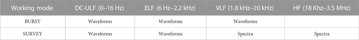
TABLE 1. Data products under different working modes.

2.2 Data selection

Earthquakes affect the ionosphere very rapidly. Generally, the larger the magnitude, the easier it is to observe pre-earthquake ionospheric anomalies. For this reason, this study uses earthquake data published on the USGS website (https://earthquake.usgs.gov/earthquakes/search/, accessed on 1st February 2022) for earthquakes of magnitude not less than 5.0 in the 3-year period from 2019 to 2021. Electromagnetic radiation generated by rock rupture is difficult to radiate from deeper underground, so earthquakes with a source depth of less than 40 km are selected (Ouyang et al., 2019).

Also, considering the complex ionospheric disturbances at high latitudes (He et al., 2020), only earthquakes occurring at low and middle latitudes were selected, and those with the south and north latitudes not less than 50° were discarded. To improve the reliability of the calculation results, only the main earthquake was considered. The earthquakes with the largest magnitude within a distribution range of ±2° in latitude and longitude and ±15 days in time were selected. After such screening of data, the final seismic library includes 2,329 seismic events, of which geographical distribution is shown in Figure 1.

FIGURE 1

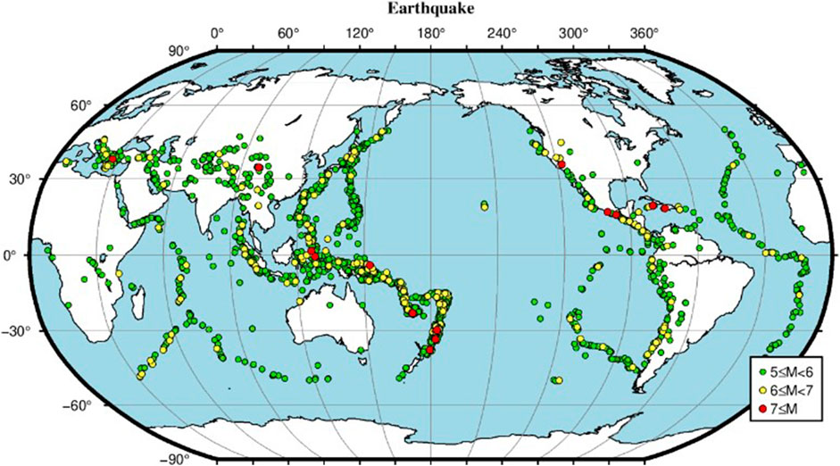
FIGURE 1. Global earthquake distribution in 2019–2021. In this figure, the green dots indicate earthquakes of magnitude five to six, the yellow dots indicate earthquakes of magnitude six to seven, and the red dots indicate earthquakes of magnitude seven or higher.

To determine the spatial and temporal extent of ionospheric anomalous disturbances caused by seismic events, the correlation between the magnitude of the earthquake and the extent of the effect on ionospheric anomalies, as well as the comparability of statistical results, are considered in determining the spatial extent. The size of the seismic zone can be calculated according to Eq. 1.

$R={10}^{0.43M}(1)$

where R represents the radius of the seismic zone in km, M represents the magnitude of the earthquake (Dobrovolsky et al., 1979). Based on previous experience, this formula can be used to estimate the areas where anomalies may occur theoretically (De Santis et al., 2019; Zheng et al., 2022). The study area was chosen to have a radius of 1,000 km centered on the epicenter.

For the selection of the time range, the time range was calculated according to the rule of the operation period of Zhangheng-1 satellite and the empirical Eq. 2 between the earthquake magnitude and the anomaly time.

$d={10}^{-3}\times M^{4.9}(2)$

where d is the number of days and M represents the magnitude of the earthquake (Hu et al., 2020). Accordingly, 15 days before to 5 days after the earthquake are chosen as the study period.

To avoid the interference of statistical results caused by anomalies due to excessive geomagnetic activity, it is set that when the average geomagnetic activity index Kp > 3 in the day when the disturbance occurs, all orbital data of that day are removed. To exclude the interference caused by solar activity and other factors on the ionosphere, the night-side data of the electric field recorded by the CSES satellite are selected for the study.

In order to interpret anomalies more objectively and to gain a comprehensive understanding of seismic ionospheric phenomena, the observed anomalies need to be verified. In statistical studies of seismic ionospheric phenomena, the random event test method is often used to test the validity of statistical results (Li, 2020; Ouyang et al., 2020). The events generation does not simply rely on generating sequence of random seismic events, but following certain rules to ensure the validity of random events. To avoid the influence of seasonal factors on the ionosphere, this study ensures that the random earthquake time is within the same seasonal range as the actual seismic event by pushing the actual earthquake 1 month ahead; meanwhile, to avoid the complex electromagnetic interference in high latitudes, only the longitude of the actual earthquake is shifted 30° westward, so that the random earthquake and the actual earthquake remain in a similar ionospheric environment (Li and Parrot, 2013).

3 Automatic detection method of ULF disturbance anomalies

During the operation of the satellite, as the EFD cuts the Earth’s magnetic lines of force, it makes the V×B additional electric field on the basis of the original electric field (Ouyang and Shen, 2015a). In addition, electromagnetic satellites work in the ionosphere and are susceptible to interference from both above (solar activity, etc.) and below (lithosphere, human activity, etc.) (He et al., 2020). This all affects the observed data. In order to remove these noise factors and to obtain the true perturbation of the ULF electric field, the empirical mode decomposition (EMD) and sample entropy based algorithm proposed by Li et al. (2022a) is optimized and used. As a result, the automatic identification of anomalous disturbances in ultra-low frequency electric fields is achieved.

The detailed process of the automatic detection method for ULF disturbance anomalies is as follows. Firstly, the original signal is decomposed. The EMD decomposition is performed on the original signal of the ULF waveform. The EMD decomposition algorithm, as an adaptive data processing method, is suitable for feature extraction of non-linear and non-stationary time series, and the original signal is decomposed and then reconstructed, so that the variation of the signal can be amplified (Huang et al., 1998; Papadopoulou and Skordas, 2014). The EMD decomposition algorithm uses the time-scale characteristics of the signal itself to decompose the signal, and any complex signal can be decomposed into a number of Intrinsic Mode Functions (IMF) that are different from each other and a residual signal. Each IMF carries information about local features of the original information at different time scales (Lu and Wang, 2021). Each IMF must satisfy the following requirements. 1) The extreme points in the original data series differ by at most one point from when they pass zero. 2) At any time, the average envelope defined by the local maximum and minimum of the signal is zero.

The EMD decomposition algorithm is shown in Eq. 3.

$S={\displaystyle \sum _{j=1}^n{c}_j}+r(3)$

where S is the original signal, n is the number of IMF components obtained by decomposition, c_j is the jth IMF component, and r is the residual signal, representing the average trend of the signal.

Secondly, the signal is reconstructed. In order to capture the anomalous information that exists as much as possible and extract the decomposed anomalous feature signals, the sample entropy is used to evaluate the complexity of each IMF obtained by EMD decomposition. Sample entropy is a new measure of time series complexity proposed by Richman and Moorman (2000), with better estimation than simple time-domain statistics. It is a commonly used method to calculate entropy values without coarse-grained extraction for original data processing and with high interference resistance. The higher the sample entropy, the higher the complexity of the time series signal and the higher the probability of carrying an implied anomalous information signal. The sample entropy of each IMF after EMD decomposition is calculated, and then the mean value of the sample entropy of all IMFs is calculated and taken as the base value, and the IMF sequences with sample entropy not less than the base value are selected for reconstruction, which can effectively reduce the error sources. After the original signal is decomposed by EMD and reconstructed by sample entropy, the trend signal of the electric field can be effectively removed from the spatial electric field waveform data to obtain the real electric field information, thus clearly depicting the anomalous change information.

Thirdly, the noise signal is removed. The factors that cause ionospheric, disturbances are complex and diverse, and not all the anomalies observed by satellites are caused by earthquakes; geomagnetic activity, solar activity, acoustic heavy waves, ionospheric disturbance transport, changes in plasma dynamics, and large-scale meteorological activity may cause ionospheric disturbances (Parrot, 2011). For this purpose the reconstructed signal is smoothed using the S-G filtering method to obtain a weighted moving average of the original data to reduce the effect of some noise on the signal (Savitzky and Golay, 1964; Li, 2015).

Finally, anomalous values are automatically identified. After the electric field disturbance anomaly signal obtained from the above steps, further determination of the disturbance anomaly value is required. 1) The magnitude of the outliers must exceed 3 times the standard deviation. 2) In order to avoid recording some non-anomalous signals, such as pulsed anomalous disturbances caused by data bursts or satellite calibration signals, only disturbance anomalies with anomaly duration up to three consecutive sampling points, about 6.144 s, are recorded, and the satellite flies about 50 km during this time, thus avoiding recording some non-anomalous signals, such as pulsed anomalous disturbances caused by data bursts or satellite calibration signals.

For example, a 7.7 magnitude earthquake (78.79°W longitude, 19.46°N latitude) that occurred in the southern waters of Cuba on 28th January 2020, is processed using an automatic detection method for ultra-low frequency disturbances. Figure 2 shows the observation results of orbit 10,823 before the earthquake.

FIGURE 2

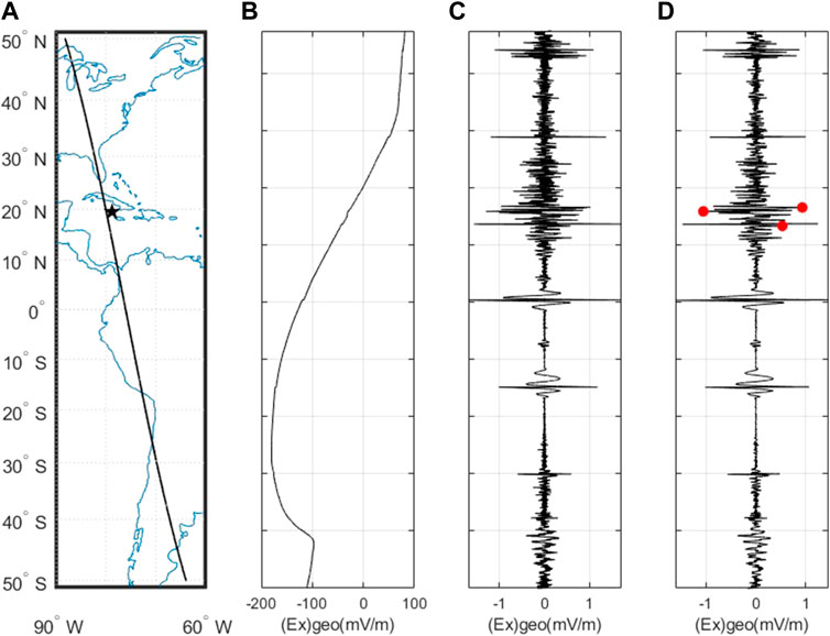
FIGURE 2. Pre-earthquake ULF disturbances in Cuba recorded by CSES orbit of 10,823. Subgraph (A) shows the area through which the satellite orbit passes, and the black pentagons represents the epicenter location; subgraph (B) shows the electric field Ex component electric field value observed by the electric field detector, and subgraph (C) shows the results of the first two steps of the automatic ultra-low frequency disturbance detection method: the real electric field signal after EMD decomposition and recombination. And subgraph (D) shows the smooth electric field signal after one S-G filtering, and the red dots represent the anomalies that exceed the determined threshold.

From Figure 2C, it can be seen that there are multiple waveform perturbations in the track, but it is difficult to identify which of the many perturbations are caused by the earthquake, which requires the discrimination of the anomalies. From Figure 2D, it can be seen that the automatic detection method of ultra-low frequency disturbances detects anomalies near the epicenter, while at the same time the index values of spatial environment such as Kp, Dst and F10.7 before and after the earthquake are at normal levels, so it can be assumed that the anomalies appearing at the epicenter may be caused by the earthquake.

4 Statistical results and analysis

The process of earthquake generation is a complex geophysical-chemical process, and the resulting anomalous manifestations are therefore also complex and diverse. The following statistics will be made on the relationship between seismic events and ULF electric field anomalies from the perspectives of time and space distribution of disturbance anomalies. By analyzing the statistical results of multiple earthquake events, it is expected that the general expression of abnormal disturbance before earthquakes will be obtained.

4.1 Multi-seismic event spatio-temporal superposed epoch analysis

4.1.1 Comparison of real and random seismic events

To investigate the correlation between earthquakes and ultra-low frequency disturbances of the electric field, superposed epoch analysis method is used to highlight the weak but critical information components from the complex background information (Hayakawa et al., 2010; Kon et al., 2011). In the superposed epoch analysis method, each grid is divided into a 12 h × 200 km spatio-temporal scale, and the Density is defined as the number of anomalies per square kilometer. Using the anomaly automatic detection algorithm introduced above, the ULF electric field data of CSES for a total of 3 years from 2019 to 2021 were scanned to obtain 49,883 ULF disturbance anomalous events; then the time difference and distance difference between each anomalous event and the earthquakes that occurred in the same period were counted and put into the divided grid; afterwards, the generated random earthquake sequences were compared with the real earthquake sequences by superposed epoch analysis. Of all the ultra-low frequency disturbances, 26,879 anomalies were related to actual earthquakes, accounting for 53% of the total anomalies detected, and 15,906 anomalies were related to random earthquakes, accounting for 31% of the total. In the statistics of real earthquake events, 213 real earthquake events have not found abnormal phenomena, accounting for 9.14% of all real earthquake events.

From Figure 3A, it can be seen that among the 2,329 earthquakes of magnitude not less than 5.0, the anomalies were concentrated within 200 km from the epicenter in terms of the spatial extent of the disturbance anomalies. Anomalous disturbances were also observed after the earthquake, indicating that electromagnetic anomalies generated during the earthquake from conception to occurrence can persist for some time after the earthquake. It is also clear from the figure that the electromagnetic anomalies associated with the earthquake were concentrated before the earthquake, and no concentration of anomalies was found on the day of the earthquake. As shown in Figure 3B, there is no significant correlation between random earthquakes and ULF perturbations of the spatial electric field, and no concentration of pre-earthquake anomalies is observed in the spatial and temporal range. The statistical results for the pseudo seismic events show that there is a significant correlation between the ULF perturbation anomalies and the real earthquakes.

FIGURE 3

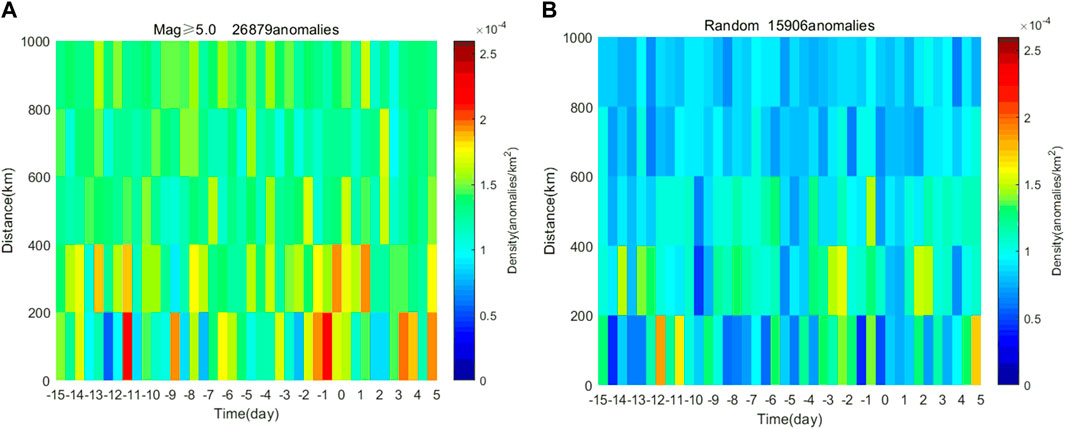
FIGURE 3. Comparison of spatial-temporal superposed epoch analysis of ULF disturbances of real and random seismic electric fields, where subgraph (A) are real earthquakes, (B) are random earthquakes, the horizontal axis indicates the time difference between the anomaly and the time of the earthquake, and the vertical axis indicates the distance between the anomaly and the epicenter.

4.1.2 Comparative analysis of spatial and temporal statistics of marine earthquakes and land earthquakes

It is experimentally proven that ULF signals are generated during rock rupture. The ULF signals generated by earthquakes propagate upward through different media and produce different observations. Therefore, it is necessary to count sea earthquakes and land earthquakes separately. Among the earthquake examples used in this experiment, 1,829 earthquakes in sea area and 500 earthquakes on land are included. The results of the superimposed ephemeral element comparison analysis of the classification statistics of sea earthquakes and land earthquakes are shown in Figure 4.

FIGURE 4

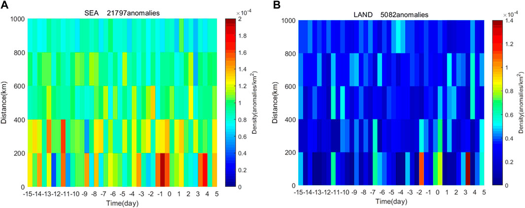
FIGURE 4. Statistical comparison of spatial-temporal superposed epoch analysis of sea earthquakes and land earthquakes. The subgraph (A) represent sea earthquakes, (B) represent land earthquakes, the horizontal axis represents the time difference between the disturbance anomaly and the earthquake, and the vertical axis represents the distance between the anomaly and the epicenter.

As shown in Figure 4A, the anomalies related with earthquakes in the sea area appear 13 days before the earthquake and are concentrated within 200 km from 1 day before the earthquake to the time of the earthquake. It is noteworthy that the anomalies can also be observed 4 days after the earthquake. As can be seen in Figure 4B, the electromagnetic anomalies related with land earthquakes increase only 2 days before the earthquake. Of the 1,829 earthquakes that occurred in the ocean, 21,797 electromagnetic anomalies were detected, while only 5,082 electromagnetic anomalies were related with 500 land earthquakes. It follows that earthquakes occurring in the sea are able to detect more anomalies than those occurring on land.

4.1.3 Spatial and temporal statistical analysis of different earthquake magnitudes

Previous studies have shown that the larger the magnitude of the earthquake is, the wider the range and more frequent the occurrence of spatial electric field disturbance anomalies are, and the easier the anomalies are to be observed (Zhang et al., 2012). In this paper, earthquakes are classified into two categories according to their magnitude: one is earthquakes of magnitude five to six and the other is earthquakes of magnitude six and above. The earthquake catalog of this study includes 2,090 earthquakes of magnitude five to six and 239 earthquakes of magnitude six and above. The results of the spatio-temporal superposition ephemeral analysis of these two types of earthquakes and the comparative analysis are shown in Figure 5.

FIGURE 5

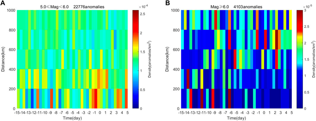
FIGURE 5. Statistical comparison of spatial-temporal superposed epoch analysis for earthquakes of different magnitudes, The subgraph (A) represents earthquakes of magnitude from five to six, subgraph (B) represents earthquakes of magnitude not less than six. The horizontal axis represents the time difference between the anomaly and the earthquake, and the vertical axis represents the distance between the anomaly and the epicenter.

Figure 5 shows there is correlation between the spatial and temporal extent of the concentrated appearance of pre-earthquake electromagnetic anomalies and the magnitude of the earthquake. In Figure 5A, most of the electromagnetic anomalies appear within 200 km from the epicenter, and the anomalies decrease substantially at 400 km from the epicenter; the anomalies appear within two satellite operation cycles, i.e., 10 days before the earthquake. The anomalies are most obvious within 200 km of the epicenter 1 day before the earthquake.

As shown in Figure 5B, electromagnetic anomalies associated with earthquakes of magnitude six and above can be observed 14 days before the earthquake, and the anomalies appear in a wide spatial range. The anomalies were most concentrated within 200 km 11 days before the earthquake and 6 days before the earthquake, while those 1 day before the earthquake were concentrated at 800 km from the epicenter.

4.2 Statistical analysis of the spatial distribution of multiple seismic events

In the spatio-temporal superposed epoch analysis of multiple seismic events, it is found that the ULF anomalous disturbances related with earthquakes are mainly concentrated in the spatial range within 200 km, while it is not clear in which direction they appear. As a result, a study area is divided into every 200 km outward with the epicenter as the center, and the orientation of anomalies appearing within each area is further investigated. To highlight the spatial electric field ULF anomalous perturbations detected before the earthquake, the time range is chosen from 15 days before the earthquake to the time of the earthquake. Figure 6 shows the statistical map of the spatial distribution of anomalies for real earthquakes of magnitude not less than 5.0.

FIGURE 6

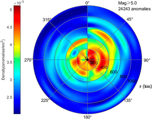
FIGURE 6. Spatial distribution statistics of ULF disturbances in the spatial electric field of earthquakes of magnitude not less than 5.0 (black pentagrams represent epicenters).

In Figure 6, the ULF disturbances are mainly concentrated within 200 km south east of the epicenter, and a significant concentration of anomalies can also be observed in a 400 km range to the southeast. The concentration of anomalies near the epicenter indicates a close coupling between seismic events and ionospheric disturbance anomalies, and a strong correlation between the appearance of anomalies and earthquakes.

4.2.1 Comparative analysis of the spatial distribution of sea earthquakes and land earthquakes

In the spatial and temporal statistical comparison of earthquakes in sea and land, it was found that the pre-seismic anomalies appear earlier in the period of sea earthquakes compared with land earthquakes. The following studies the spatial distribution characteristics of anomalies from the perspective of earthquakes in different regions, and the statistical results are shown in Figure 7.

FIGURE 7

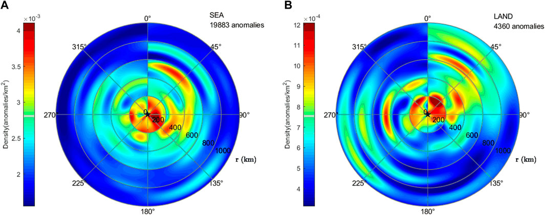
FIGURE 7. Statistical comparison of the spatial distribution of seismic anomalies in the sea and on land (black pentagrams represent epicenters).

Figure 7A shows the statistical map of the spatial distribution of anomalies for earthquakes in the sea. It can be seen that the anomalies related to earthquakes occurred in the sea are mainly distributed within 200 km in the southeast. Figure 7B shows the spatial distribution of anomalies for earthquakes on land. The locations of ULF signal anomalies are more dispersed and widely distributed, but most of them appear in the north side of the epicenter. It can be seen from the comparative analysis that the ionospheric disturbance related with the earthquake occurred in the sea area is closer to the epicenter. The reason may be that the electromagnetic wave propagation medium of marine earthquakes is single. However, when the electromagnetic wave of land earthquake propagates from the underground to the surface to the ionosphere, it is easy to be absorbed due to encountering multiple media, making the initial weak signal of earthquake preparation unable to reach the ionosphere, which leads to this phenomenon.

4.2.2 Comparison of statistical analysis of spatial distribution of different earthquake levels

Analysis of the spatial and temporal statistical results for different earthquake magnitudes reveals that the larger the magnitude is, the earlier the ULF signal disturbance anomalies appear. The spatial distribution characteristics of earthquakes of magnitude five to six and not less than six are discussed below, and the statistical results are shown in Figure 8.

FIGURE 8

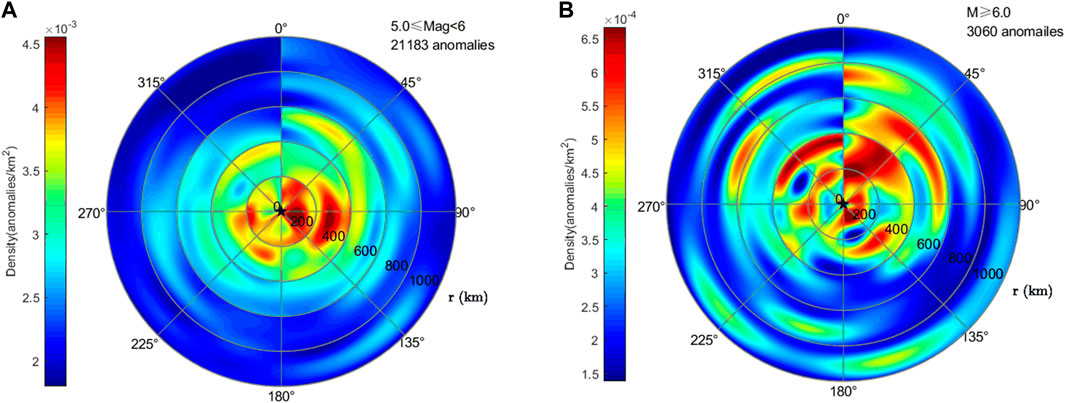
FIGURE 8. Statistical comparison of the spatial distribution of different earthquake magnitudes (black pentagons represent epicenters).

Figure 8A shows the spatial distribution of disturbance anomalies for magnitude five to six earthquakes, and subplot Figure 8B shows the spatial distribution of disturbance anomalies for magnitude not less than six earthquakes. As shown in subgraph Figure 8A, the 5–6 earthquake anomalies mainly appear on the east side of the epicenter within 400 km from the epicenter, and are mostly concentrated within 200 km. As the magnitude of the earthquake increases, the anomalies appear in a scattered range, and can be observed within 1,000 km from the epicenter, as shown in Figure 8B. It is noteworthy that almost all the anomalies farther away from the epicenter appear in the north side of the epicenter, and can only be observed within 400 km in the south side of the epicenter. This indicates that the range of the anomalies caused by the earthquake increases with the increase of the magnitude.

4.2.3 Comparison of statistical analysis of spatial distribution in the northern and southern hemispheres

It is generally accepted in previous earthquake studies that the electromagnetic anomalies caused by earthquakes are usually shifted in the direction of the magnetic equator, not exactly directly above the epicenter because of the Earth’s magnetic field (Pulinets and Legen’ka, 2003). Therefore, it is possible to divide the northern and southern hemisphere comparisons according to the location of earthquake occurrence, with 1,076 earthquakes in the northern hemisphere and 1,253 in the southern hemisphere. The statistical results of the spatial distribution of the northern and southern hemispheres are shown in Figure 9.

FIGURE 9

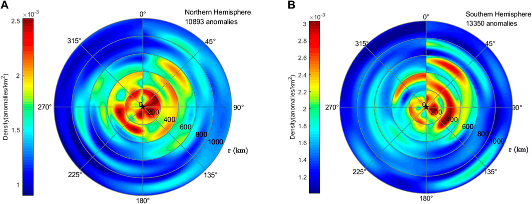
FIGURE 9. Statistical analysis of spatial distribution in the northern and southern hemispheres (black asterisks represent epicenters).

As shown in Figure 9A, the east concentration of anomalies in seismic events occurring in the northern hemisphere occurs in the region south of the epicenter; in Figure 9B, the anomalies are mainly concentrated in the eastern side for earthquakes occurring in the southern hemisphere. Previous studies have shown that ionospheric anomalies caused by earthquakes are usually shifted along the geomagnetic magnetic line of force toward the geomagnetic equator, a phenomenon that is consistent with the spatial statistical distribution of earthquakes in the Northern Hemisphere but not in the Southern Hemisphere.

5 Discussion and conclusion

5.1 Discussion

The statistical results in this study demonstrate that the occurrence of seismic anomalies of magnitude not less than 5.0 was within 200 km from the epicenter in about 11 days before and 2 days before to 12 h before the earthquake. In addition, we found a noteworthy that there was no concentration of anomalies found on the day of the earthquake, a situation that has been reported in many previous studies (Boudjada et al., 2010; Georgios et al., 2012), This phenomenon will be a major part of our future research. Among the earthquake cases studied, 87% of the earthquakes were of magnitude 5–6, according to the earthquake preparation zone formula, it is reasonable that the range of anomalies generated during the earthquake incubation process is concentrated within 400 km, with the most obvious within 200 km. Interestingly, the appearance of anomalous disturbances was also found after the earthquake, which may be due to the tectonic plates still colliding with each other after the main earthquake. Moreover, eighty percent of the earthquake cases in this study occurred in the sea, and secondary hazards such as tsunamis and volcanic eruptions caused by the earthquake can also lead to ionospheric disturbances (Jin et al., 2010; Hao et al., 2012). Earthquakes are generated by the collision and compression of tectonic plates against each other, and the displacement and faulting caused by earthquakes may also cause ionospheric disturbances in the post-earthquake crustal recovery process. In this regard, there is no in-depth analysis in this study, and further research is needed.

From the spatial perspective, the anomalies related with the sea earthquakes were mainly concentrated in the spatial range within 200 km from the epicenter, while those related with the land earthquakes were more scattered; temporally, the anomalies related with the sea earthquakes appeared several times before the earthquake. Moreover, the average number of anomalies related with each sea earthquake we counted was more than that related with each land earthquake, so it is considered that more anomalies can be observed for sea earthquakes.

In the classification statistics of earthquake magnitude, it is found that although earthquakes of magnitude six or higher can be observed in a larger spatial and temporal scale, the statistics of anomalies within 200 km of the epicenter in one cycle before the earthquake are not prominent. The reason for this result is, on the one hand, that the effects of earthquakes with larger magnitude can be observed in a large spatial scale; on the other hand, it may be that there are too few earthquake cases, which leads to insufficient observation results; additionally, since the satellite is observing in motion, it is difficult to make a complete observation of the gestation process of each earthquake case, which may also lead to this result. In future studies, it is necessary to improve the anomaly identification method, accumulate more earthquake cases, conduct finer classification and classification studies, and carry out joint studies of multiple satellites to make up for the shortcomings in this regard.

5.2 Conclusion

In this study, the electric field ULF data observed by CSES in 2019–2021 are used for analysis, 26,879 ULF disturbance events related with earthquakes are identified from 2,329 earthquakes of magnitude not less than 5.0 using the automatic ULF disturbance algorithm, followed by a superposed epoch analysis. The study was conducted both temporally and spatially, with analyze of spatial distribution characteristics, and the following four conclusions are obtained from the statistical analysis according to earthquake location and earthquake magnitude respectively.

(1) By superposed epoch analysis and random event test for earthquakes of magnitude not less than 5.0, it is demonstrated that ULF disturbance events are highly correlated with earthquakes.

(2) From the spatial and temporal statistics, the anomalous disturbances of earthquakes of magnitude not less than 5.0 usually appear 11 to 2 days before the occurrence of the earthquake. In terms of spatial distribution characteristics, the earthquake-related anomalies are mainly concentrated within 200 km to the south-east of the epicenter.

(3) Sea earthquakes can observe more pre-seismic anomalous electromagnetic disturbances than land earthquakes.

(4) With the increase of earthquake magnitudes, the anomalies tend to appear earlier and are distributed more widely.

Data availability statement

The datasets presented in this study can be found in online repositories. The names of the repository/repositories and accession number(s) can be found below: https://leos.ac.cn; http://wdc.kugi.kyoto-u.ac.jp/dstae/index.html; https://earthquake.usgs.gov/earthquakes/search/.

Author contributions

B-YY contributed to algorithm implementation. ZL contributed to the conceptualization and methodology. X-MY contributed to software. J-PH contributed to data analysis and conclusion. Z-YL wrote the original draft. H-CY reviewed and edited manuscript. Z-YL contributed to resources. W-JL contributed to validation. X-HS contributed to supervision. ZZ and QT contributed to data curation. NN contributed to investigation. All authors read and approved the final manuscript.

Funding

This research was funded by Open Project Fund of Hebei Key Laboratory of Seismic Disaster Instrument and Monitoring Technology (No. FZ224104). The National Natural Science Foundation of China (No. 42104159), the APSCO Earthquake Special Project II, and ISSI-BJ2019. This work made use of the data from the CSES mission, a project funded by China National Space Administration (CNSA) and the China Earthquake Administration (CEA).

Acknowledgments

Thanks to the CSES satellite team for the data (https://leos.ac.cn, accessed on 1st February 2022). Thanks to the World Data Center for Geomagnetism. The geomagnetic index data can be found here: (http://wdc.kugi.kyoto-u.ac.jp/dstae/index.html, accessed on 1st February 2022). Thanks to USGS for Earthquake catalogue (https://earthquake.usgs.gov/earthquakes/search/ accessed, on 1st February 2022).

Conflict of interest

The authors declare that the research was conducted in the absence of any commercial or financial relationships that could be construed as a potential conflict of interest.

Publisher’s note

All claims expressed in this article are solely those of the authors and do not necessarily represent those of their affiliated organizations, or those of the publisher, the editors and the reviewers. Any product that may be evaluated in this article, or claim that may be made by its manufacturer, is not guaranteed or endorsed by the publisher.

References

Adib, Y. K., Mardina, A., Abdul, H. N. S., Suaidi, A., and Akimasa, Y. (2021). Correlations between earthquake properties and characteristics of possible ULF geomagnetic precursor over multiple earthquakes. Universe 7 20(1). doi:10.3390/UNIVERSE7010020

CrossRef Full Text | Google Scholar

Błeçki, J., Parrot, M., and Wronowski, R. (2010). Studies of the electromagnetic field variations in ELF frequency range registered by DEMETER over the Sichuan region prior to the 12 May 2008 earthquake. Int. J. Remote Sens. 31 (13), 3615–3629. doi:10.1080/01431161003727754

CrossRef Full Text | Google Scholar

Boudjada, M. Y., Schwingenschuh, K., Döller, R., Rohznoi, A., Parrot, M., Biagi, P. F., et al. (2010). Decrease of VLF transmitter signal and Chorus-whistler waves before l'Aquila earthquake occurrence. Nat. Hazards Earth Syst. Sci. 10 (7), 1487–1494. doi:10.5194/nhess-10-1487-2010

CrossRef Full Text | Google Scholar

De Santis, A., Marchetti, D., Pavón-Carrasco, F. J., Cianchini, G., Perrone, L., Abbattista, C., et al. (2019). Precursory worldwide signatures of earthquake occurrences on Swarm satellite data. Sci. Rep. 9 (1), 20287. doi:10.1038/s41598-019-56599-1

PubMed Abstract | CrossRef Full Text | Google Scholar

Dobrovolsky, I. P., Zubkov, S. I., and Miachkin, V. I. (1979). Estimation of the size of earthquake preparation zones. Pure Appl. Geophys. 117 (5), 1025–1044. doi:10.1007/bf00876083

CrossRef Full Text | Google Scholar

Fraser-Smith, A. C., Bernardi, A., McGill, P. R., Ladd, M. E., Helliwell, R. A., and Villard, O. G. (1990). Low-frequency magnetic field measurements near the epicenter of the Ms 7.1 Loma Prieta Earthquake. Geophys. Res. Lett. 17 (9), 1465–1468. doi:10.1029/GL017i009p01465

CrossRef Full Text | Google Scholar

Georgios, C., Efthymios, V., and Sergey, P. (2012). Characteristics of flux-time profiles, temporal evolution, and spatial distribution of radiation-belt electron precipitation bursts in the upper ionosphere before great and giant earthquakes. Ann. Geophys. 55 (1). doi:10.4401/ag-5365

CrossRef Full Text | Google Scholar

Gokhberg, M. B., Morgounov, V. A., Yoshino, T., and Tomizawa, I. (1982). Experimental measurement of electromagnetic emissions possibly related to earthquakes in Japan. J. Geophys. Res. 87 (B9), 7824–7828. doi:10.1029/jb087ib09p07824

CrossRef Full Text | Google Scholar

Hao, Y., Xiao, Z., and Zhang, D. (2012). Multi-instrument observation on co-seismic ionospheric effects after great Tohoku earthquake. J. Geophys. Res. 117 doi:10.1029/2011ja017036A2).

CrossRef Full Text | Google Scholar

Hayakawa, M., Hattori, K., and Ohta, K. (2007). Monitoring of ULF (Ultra-Low-Frequency) geomagnetic variations associated with earthquakes. Sensors 7(7), 1108–1122. doi:10.3390/s7071108

CrossRef Full Text | Google Scholar

Hayakawa, M., Kasahara, Y., Nakamura, T., Muto, F., Horie, T., Maekawa, S., et al. (2010). A statistical study on the correlation between lower ionospheric perturbations as seen by subionospheric VLF/LF propagation and earthquakes. J. Geophys. Res. 115 (A9). doi:10.1029/2009JA015143

CrossRef Full Text | Google Scholar

He, Y. F., Yang, D. M., Chen, H. R., Qian, J. D., Zhu, R., and Parrot, M. (2009). Demeter satellite detected the signal-to-noise ratio change of ground VLF transmitting station signal that may be related to Wenchuan earthquake. Chin. Sci. Part D. 39 (04), 403–412. doi:10.1016/S1874-8651(10)60080-4

CrossRef Full Text | Google Scholar

He, Y. (2020). Study on seismo-ionospheric phenomena based on electric density data Record by SWARM and DEMETER satellite. Inst. Geophys. china Earthq. Adm.

Google Scholar

Hu, Y., Zhima, Z. R., Huang, J., Zhao, S., Guo, F., Wang, Q., et al. (2020). Algorithms and implementation of wave vector analysis toolfor the electromagnetic waves recorded by the CSES satellite. Chin. J.Geophys 63 (05), 1751–1765. doi:10.6038/cjg2020N0405

CrossRef Full Text | Google Scholar

Huang, J., Jia, J., Yin, H., Li, Z., Li, J., Shen, X., et al. (2022). Study of the statistical characteristics of Artificial source signals based on the CSES. Front. Earth Sci. (Lausanne). 10. doi:10.3389/feart.2022.883836

CrossRef Full Text | Google Scholar

Huang, J., Liu, J., Ouyang, X. Y., and Li, W. (2010). Analysis to the energetic particles around the m8.8 chili earthquake. Seismol. Geol. 32 (03), 417–423. doi:10.3969/j.issn.0253-4967.2010.03.008

CrossRef Full Text | Google Scholar

Huang, N. E., Shen, Z., Long, S. R., Wu, M. C., Shih, H. H., Zheng, Q., et al. (1998). The empirical mode decomposition and the Hilbert spectrum for nonlinear and non-stationary time series analysis. Proc. R. Soc. Lond. A 454(1971), 903–995. doi:10.1098/rspa.1998.0193

CrossRef Full Text | Google Scholar

Jin, S., Zhu, W., and Afraimovich, E. (2010). Co-seismic ionospheric and deformation signals on the 2008 magnitude 8.0 Wenchuan Earthquake from GPS observations. Int. J. Remote Sens. 31 (13), 3535–3543. doi:10.1080/01431161003727739

CrossRef Full Text | Google Scholar

Kon, S., Nishihashi, M., and Hattori, K. (2011). Ionospheric anomalies possibly associated with M⩾ 6.0 earthquakes in the Japan area during 1998–2010: Case studies and statistical study. J. Asian Earth Sci. 41 (4-5), 410–420. doi:10.1016/j.jseaes.2010.10.005

CrossRef Full Text | Google Scholar

Li, K. (2020). Pre-earthquake anomaly detection and statistical analysis of Swarm Sate-llite magnetic field data. Changchun, China: jilin university.

Google Scholar

Li, M., and Parrot, M. (2013). Statistical analysis of an ionospheric parameter as a base for earthquake prediction. J. Geophys. Res. Space Phys. 118 (6), 3731–3739. doi:10.1002/jgra.50313

CrossRef Full Text | Google Scholar

Li, M. (2015). Statistical characteristics of seismic influence on Ionosphereand study of Earth一atmosphere electromagnetic coupling Besed on the Wenchuan Ms8.0 earthquake. Beijing): China University of Geosciences.

Google Scholar

Li, M., Shen, X., Parrot, M., Zhang, X., Zhang, Y., Yu, C., et al. (2020). Primary joint statistical seismic influence on ionospheric parameters recorded by the CSES and DEMETER satellites. JGR. Space Phys. 125 (12). doi:10.1029/2020JA028116

CrossRef Full Text | Google Scholar

Li, Z., Song, Y., Liu, H., and An, J. (2018). Review of the earthquake electromagnetic precursor research based on groundand space observations. Chin. J. radio Sci. 33 (01), 105–115. doi:10.13443/j.cjors.2017072101

CrossRef Full Text | Google Scholar

Li, Z., Li, J., Huang, J., Yin, H., and Jia, J. (2022a). Research on pre-seismic feature Recognition of spatial electric field data recorded by CSES. Atmosphere 13 (2), 179. doi:10.3390/atmos13020179

CrossRef Full Text | Google Scholar

Li, Z., Yang, B., Huang, J., Yin, H., Yang, X., Liu, H., et al. (2022b). Analysis of pre-earthquake space electric field disturbance observed by CSES. Atmosphere 13 (6), 934. doi:10.3390/atmos13060934

CrossRef Full Text | Google Scholar

Lu, J., and Wang, Z. (2021). The Systematic Bias of entropy calculation in the Multi-scale entropy algorithm. Entropy 23 (6), 659, doi:10.3390/e23060659

PubMed Abstract | CrossRef Full Text | Google Scholar

Akhoondzadeh, M. (2013). Novelty detection in time series of ULF magnetic and electric components obtained from DEMETER satellite experiments above Samoa (29 September 2009) earthquake region. Nat. Hazards Earth Syst. Sci. 13 15, 25. doi:10.5194/nhess-13-15-2013169).

CrossRef Full Text | Google Scholar

Ma, M., Lei, J., Li, C., Li, S., Zong, C., Liu, Z., et al. (2018). Design Optimization of Zhangheng-1 space electric field detector. Chin. J. vacuuum Sci. Technol. 38 (07), 582–589. doi:10.13922/j.cnki.cjovst.2018.07.06

CrossRef Full Text | Google Scholar

Ouyang, X. Y., and Shen, X. (2015a). Method for pre-processing ULF electric field disturbances observed by DEMETER and its case application analysis. Acta Seismol. sin. 37 (05), 820–829. doi:10.11939/jass.2015.05.010

CrossRef Full Text | Google Scholar

Ouyang, X. Y., and Shen, X. (2015b). Typical interferences of ULF electric field waveform data observed by DEMETER. Seismol. geomagnetic observation Res. 36 (4), 19–25.

Google Scholar

Ouyang, X., Bortnik, J., Ren, J., and Berthelier, J. (2019). Features of Nightside ULF wave activity in the ionosphere. J. Geophys. Res. Space Phys. 124 9203, 9213. doi:10.1029/2019ja02710311).

CrossRef Full Text | Google Scholar

Ouyang, X. Y., Parrot, M., and Bortnik, J. (2020). ULF wave activity observed in the nighttime ionosphere above and some Hours before strong earthquakes. J. Geophys. Res. Space Phys. 125 doi:10.1029/2020ja0283969).

CrossRef Full Text | Google Scholar

Papadopoulou, K. A., and Skordas, E. S. (2014). Application of the Huang-Hilbert transform and natural time to the analysis of seismic electric signal activities. Chaos. 24 (4), 043102. doi:10.1063/1.4896795

PubMed Abstract | CrossRef Full Text | Google Scholar

Parrot, M. (2011). Statistical analysis of the ion density measured by the satellite DEMETER in relation with the seismic activity. Earthq. Sci. 24 (06), 513–521. doi:10.1007/s11589-011-0813-3

CrossRef Full Text | Google Scholar

Píša, D., Němec, F., Santolík, O., Parrot, M., and Rycroft, M. (2013). Additional attenuation of natural VLF electromagnetic waves observed by the DEMETER spacecraft resulting from preseismic activity. J. Geophys. Res. Space Phys. 118 (8), 5286–5295. doi:10.1002/jgra.50469

CrossRef Full Text | Google Scholar

Pulinets, S. A., and Legen'ka, A. D. (2003). Spatial–temporal characteristics of large scale disturbances of electron density observed in the ionospheric F-region before strong earthquakes. Cosmic Res. 41 (3), 221–230. doi:10.1023/A:1024046814173

CrossRef Full Text | Google Scholar

Richman, J. S., and Moorman, J. R. (2000). Physiological time-series analysis using approximate entropy and sample entropy. Am. J. Physiology-Heart Circulatory Physiology 278 (6), H2039–H2049. doi:10.1152/ajpheart.2000.278.6.H2039

PubMed Abstract | CrossRef Full Text | Google Scholar

Sarkar, S., and Gwal, A. K. (2010). Satellite monitoring of anomalous effects in the ionosphere related to the great Wenchuan earthquake of May 12, 2008. Nat. Hazards (Dordr). 55 (2), 321–332. doi:10.1007/s11069-010-9530-9

CrossRef Full Text | Google Scholar

Sarlis, N. V. (2018). Statistical significance of Earth’s electric and magnetic field variations preceding earthquakes in Greece and Japan revisited. Entropy 20 (8), 561, doi:10.3390/e20080561

PubMed Abstract | CrossRef Full Text | Google Scholar

Savitzky, A., and Golay, M. (1964). Smoothing and Differentiation of data by Simplified Least squares Procedures. Anal. Chem. 36 (8), 1627–1639. doi:10.1021/ac60214a047

CrossRef Full Text | Google Scholar

Serebryakova, O. N., Bilichenko, S. V., Chmyrev, V. M., Parrot, M., Rauch, J. L., Lefeuvre, F., et al. (2013). Electromagnetic ELF radiation from earthquake regions as observed by low-altitude satellites. Geophys. Res. Lett. 19 (2), 91–94. doi:10.1029/91gl02775

CrossRef Full Text | Google Scholar

Slifkin, L. (1993). Seismic electric signals from displacement of charged dislocations. Tectonophysics 224 (1), 149–152. doi:10.1016/0040-1951(93)90066-S

CrossRef Full Text | Google Scholar

Solovieva, M. S., Rozhnoi, A. A., and Molchanov, O. A. (2009). Variations in the parameters of VLF signals on the DEMETER satellite during the periods of seismic activity. Geomagn. Aeron. 49 (4), 532–541. doi:10.1134/S0016793209040161

CrossRef Full Text | Google Scholar

Uyeda, S., Nagao, T., and Kamogawa, M. (2009). Short-term earthquake prediction: Current status of seismo-electromagnetics. Tectonophysics 470 (3), 205–213. doi:10.1016/j.tecto.2008.07.019

CrossRef Full Text | Google Scholar

Uyeda, S., Nagao, T., Orihara, Y., Yamaguchi, T., and Takahashi, I. (2000). Geoelectric potential changes: Possible precursors to earthquakes in Japan. Proc. Natl. Acad. Sci. U. S. A. 97(9), 4561–4566. doi:10.1073/pnas.97.9.4561

PubMed Abstract | CrossRef Full Text | Google Scholar

Varotsos, P., and Alexopoulos, K. (1984). Physical properties of the variations of the electric field of the Earth preceding earthquakes. Tectonophys 110 (1), 73–98. doi:10.1016/0040-1951(84)90059-3

CrossRef Full Text | Google Scholar

Varotsos, P., and Lazaridou, M. (1991). Latest aspects of earthquake prediction in Greece based on seismic electric signals. Tectonophysics 188 (3), 321–347. doi:10.1016/0040-1951(91)90462-2

CrossRef Full Text | Google Scholar

Varotsos, P. A., Sarlis, N. V., and Skordas, E. S. (2003). Electric fields that “Arrive” before the time Derivative of the magnetic field prior to major earthquakes. Phys. Rev. Lett. 91 (14), 148501. doi:10.1103/PhysRevLett.91.148501

PubMed Abstract | CrossRef Full Text | Google Scholar

Walker, S. N., Kadirkamanathan, V., and Pokhotelov, O. A. (2013). Changes in the ultra-low frequency wave field during the precursor phase to the Sichuan earthquake: DEMETER observations. Ann. Geophys. 31 1597, 1603. doi:10.5194/angeo-31-1597-20139).

CrossRef Full Text | Google Scholar

Yan, R., Wang, L., Hu, Z., Liu, D., Zhang, X., and Zhang, Y. (2013). Ionospheric disturbances before and after strong earthquakes based on DEMETER data. Acta Seismol. sin. (04), 498–511. doi:10.3969/j.issn.0253-3782.2013.04.005

CrossRef Full Text | Google Scholar

Yan, R., Parrot, M., and Pinçon, J.-L. (2017). Statistical study on variations of the ionospheric ion density observed by DEMETER and related to seismic activities. J. Geophys. Res. Space Phys. 122 (12), 12421–412429. doi:10.1002/2017JA024623

CrossRef Full Text | Google Scholar

Yang, C., Yong, S., Wang, X., and Liu, C. (2021). Research on Indonesia Ms 7.4 earthquake based on data of Zhangheng-1 electromagnetic satellite. Acta Sci. Nat. Univ. Pekin. 57 (06), 997–1005. doi:10.13209/j.0479-8023.2021.097

CrossRef Full Text | Google Scholar

Yao, L., Shen, X., and Zhang, X. (2014). Analysis of ionospheric anomalies preceding the 2010 Yushu MS7. 1 earthquake. EARTHQUAKE 34 (03), 74–85.

Google Scholar

Zhang, X., Qian, J., Ouyang, X., Shen, X., Cai, J. a., and Zhao, S. (2009a). Ionospheric electromagnetic perturbations observed on DEMETER satellite before Chile M7.9 earthquake. Earthq. Sci. 22 (3), 251–255. doi:10.1007/s11589-009-0251-7

CrossRef Full Text | Google Scholar

Zhang, X., Shen, X., Liu, J., Ouyang, X., Qian, J., and Zhao, S. (2009b). Analysis of ionospheric plasma perturbations before Wenchuan earthquake. Nat. Hazards Earth Syst. Sci. 9 (4), 1259–1266. doi:10.5194/nhess-9-1259-2009

CrossRef Full Text | Google Scholar

Zhang, X., Shen, X., Parrot, M., Zeren, Z., Ouyang, X., Liu, J., et al. (2012). Phenomena of electrostatic perturbations before strong earthquakes (2005–2010) observed on DEMETER. Nat. Hazards Earth Syst. Sci. 12 (1), 75–83. doi:10.5194/nhess-12-75-2012

CrossRef Full Text | Google Scholar

Zhang, X., Wang, Y., Boudjada, M. Y., Liu, J., Magnes, W., Zhou, Y., et al. (2020). Multi-experiment observations of ionospheric disturbances as precursory effects of the Indonesian Ms6.9 earthquake on August 05, 2018. Remote Sens. 12 (24), 4050, doi:10.3390/rs12244050

CrossRef Full Text | Google Scholar

Zheng, L., Yan, R., Parrot, M., Zhu, K., Zhima, Z., Liu, D., et al. (2022). Statistical research on seismo-ionospheric ion density Enhancements observed via DEMETER. Atmosphere 13 (8), 1252, doi:10.3390/atmos13081252

CrossRef Full Text | Google Scholar

Zhi-Ma, Z., Xu-Hui, S., Jin-Bin, C. A. O., Xue-Min, Z., Jian-Ping, H., Jing, L. I. U., et al. (2012a). Statistical analysis of ELF/VLF magnetic field disturbances before major earthquakes. Chin. J. Geophys. (in Chinese)VL - 55 (11), 3699–3708. doi:10.6038/j.issn.0001-5733.2012.11.017

CrossRef Full Text | Google Scholar

Zhima, Z., Xuhui, S., Xuemin, Z., Jinbin, C., Jianping, H., Xinyan, O., et al. (2012b). Possible ionospheric electromagnetic perturbations Induced by the Ms7.1 Yushu earthquake. Earth Moon Planets 108 231, 241. doi:10.1007/s11038-012-9393-z3-4).

CrossRef Full Text | Google Scholar

Zhu, K., Zheng, L., Yan, R., Shen, X., Zeren, Z., Xu, S., et al. (2021). The variations of electron density and temperature related to seismic activities observed by CSES. Natural Hazards Research 1 (2), 88–94. doi:10.1016/j.nhres.2021.06.001

CrossRef Full Text | Google Scholar

Zlotnicki, J., Kossobokov, V., and Le Mouël, J.-L. (2001). Frequency spectral properties of an ULF electromagnetic signal around the 21 July 1995, M=5.7, Yong Deng (China) earthquake. Tectonophysics 334 (3), 259–270. doi:10.1016/S0040-1951(00)00222-5

CrossRef Full Text | Google Scholar

Zlotnicki, J., Le Mouël, J. L., Kanwar, R., Yvetot, P., Vargemezis, G., Menny, P., et al. (2006). Ground-based electromagnetic studies combined with remote sensing based on Demeter mission: A way to monitor active faults and volcanoes. Planetary and Space Science 54 (5), 541–557. doi:10.1016/j.pss.2005.10.022

CrossRef Full Text | Google Scholar