MAFIAT: Magnetic field analysis tools

The magnetic twist is one of the key defining parameters of solar flux ropes (FRs). The routine computation of the winding of magnetic field lines, referred to as the twist, has the potential to lead to significant advancement in the field of solar physics and solar—terrestrial research, e.g., by enabling more accurate investigations of FR morphology, stability, and temporal evolution. However, this has been hampered by the axial-dependence of the solution and the availability of simpler, albeit approximate, methods. Here we introduce the Magnetic Field Analysis Tools (MAFIAT) python library and Jupyter notebooks for the computation and exploitation of this quantity. The required axis location is specified manually by the user, either with their own preferred method, or using the twist number calculated from the parallel current by Magnetic Field Analysis Tools. The notebooks allow users to create a variety of novel visualisations of FRs and their twist distributions for scientific study. Magnetic Field Analysis Tools is written in Python and is released under the BSD 3-Clause Licence. Code available at: https://github.com/pricedj/mafiat.

1 Introduction

Coronal mass ejections (CMEs; Webb and Howard, 2012) are gigantic structures of magnetic field and plasma that regularly erupt from the Sun and serve as one of the primary drivers of space weather in the heliosphere. Their study is critical due to their vast and often adverse impact, ranging from human spaceflight to national power grids and other infrastructure (e.g., Eastwood et al., 2017; Kilpua et al., 2017). An integral component of CMEs are flux ropes, helical structures where magnetic field lines wind about a common axis (Chen, 2017). The understanding of CMEs and their impact requires a detailed knowledge of their magnetic fields and their associated flux ropes (FRs), from their formation in the corona to their eventual eruption and propagation (e.g., Kilpua et al., 2019). However, directly measuring coronal magnetic fields is very difficult and as a result modelling is usually employed (Wiegelmann et al., 2017).

Flux ropes possess a number of fundamental properties that are also useful to study in their own right. Here we focus on one of the most critical parameters, the magnetic twist, which describes the number of turns that a magnetic field line makes around the FR axis. Computations of the twist sheds light on how stable the FR is, and therefore how it evolves and the likelihood of it erupting (e.g., Amari et al., 2018; Inoue et al., 2018; Zhong et al., 2021). For example, in the case of the kink instability, a FR is said to be unstable and likely to erupt if twisted beyond a critical value (Török and Kliem, 2003). There are several distinct quantities that are commonly called twist which, in general, do not measure the same thing. As a result, ‘twist’ values must always be considered alongside the methodology employed (Liu et al., 2016).

A commonly used metric for quantifying twist is the twist number T_w which uses the parallel current and magnetic field to compute how many turns two infinitesimally close field lines wind about each other (Berger and Prior, 2006, Eq. 16). A simpler quantity is T_α, computed using the force-free parameter α at the footpoints of the FR (Inoue et al., 2011). However, these methods, and others, notably do not factor in the geometry of the field lines. The twist number T_g introduced by Berger and Prior (2006) (see their Eq. 12) takes this into consideration. T_g describes how many times each field line winds about the flux rope axis. It is defined as

$T_g=\frac{1}{2\pi }{\int }_x\frac{d\phi }{ds}ds=\frac{1}{2\pi }{\int }_x\widehat{\mathbf{T}}\left(s\right)\cdot \widehat{\mathbf{V}}\left(s\right)\times \frac{d\widehat{\mathbf{V}}\left(s\right)}{ds}ds(1)$

Where x(s) defines the flux rope axis, φ the rotation angle made by the field line under consideration about x(s), $\widehat{\mathbf{T}}$ the unit tangent vector to x(s) (i.e., the local direction of the flux rope axis), and $\widehat{\mathbf{V}}$ the unit vector normal to x(s) which intersects the field line under consideration. This method is more computationally expensive and more difficult to employ, but it factors in the geometry of the FR. For a comparison of these, and other, twist methods, see Liu et al. (2016).

This paper serves to introduce the newly released collection of Magnetic Field Analysis Tools (MAFIAT). The primary purpose of MAFIAT is to compute the quantity T_g and to provide useful visualisations of its distribution throughout the flux rope.

2 Methods

2.1 Implementation

MAFIAT is designed to support the analysis of magnetic fields in coronal simulations. It is written in Python 3 and is freely available from GitHub. Additionally, it is compatible with PyPI, enabling the installation of MAFIAT, along with its dependencies, with the widely used pip command-line tool. The primary workflow is in the form of the included Jupyter Notebooks, however, the functions can also be used in scripts as desired.

The list of required dependencies is kept as short as possible to minimise the potential for compatibility issues. At present, MAFIAT requires the widely used ipykernel, k3d, matplotlib, numba, numpy, and scipy packages. Additionally, it requires the newly-released pySMSH package which provides tools for working with grid-based simulation data.

2.2 Overview

The primary workflow of MAFIAT enables the computation of T_g for flux ropes in coronal simulation domains. This consists of four main steps:

1. Data loading and initialisation

2. Computing T_w to locate the FR axis

3. Computing T_g

4. Visualising the results

The first three steps take part in the Computing_Tg notebook, and the fourth step takes place in the Visualising_Tg notebook, both provided in the notebooks folder of the repository. The following sections describe these steps in more detail.

2.2.1 Initialisation

MAFIAT requires an input file with magnetic field data and details of the corresponding Cartesian rectilinear grid. From this, magnetic field and current density interpolators are initialised to facilitate the computation of T_w and the tracing of magnetic field lines through the simulation domain.

2.2.2 Axis location

After initialisation, the user is required to select a 2D plane that is orthogonal with one of the coordinate axes. It is advised that a plane bisecting the apex of the FR is chosen as closely as possible. Following this, the compute_Tw_map function is used to calculate T_w for the chosen plane.

The plane is then processed in a series of steps to identify the flux rope and facilitate locating the axis. First, any open field lines are removed, i.e., any field lines where both ends are not rooted in the photosphere. Second, any regions of small twist number (|T_w| < 0.99) are removed. This choice provides a good estimate of FR extent in many cases, but can be changed by the user as needed. Third, if a horizontal slice (i.e., a cut in z) was made then any regions with a positive (or negative) polarity are removed so that the FR only threads the plane once. Fourth, any points with the wrong sign of T_w are removed based on user selection. The fifth, and final, step is manual trimming of any other undesired regions of T_w. The remaining region is considered to correspond to the FR and its coordinates are saved for future use. We note that none of the steps above are strictly mandatory, and can be omitted.

Next, T_w is computed again at a higher resolution, for the region defined following the previous procedure and plotted with contours to assist in identifying the axis, which is considered to be at an extremum of T_w. The user should adjust the values of the contour levels until the axis is well-defined. In practice, this can mean adjusting the values by fractional amounts in a series of trial and error. Then the centre of the axis contour is taken forward as the axis of the FR (Figure 1).

FIGURE 1

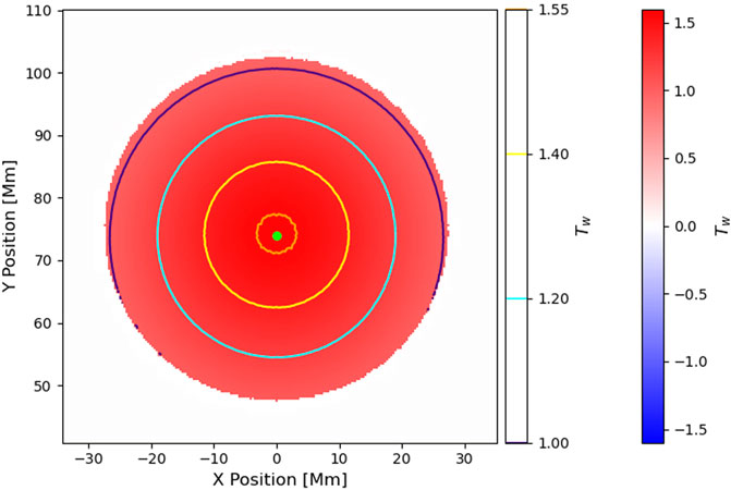
FIGURE 1. Output from the axis locating step, showing a high-resolution plot of T_w with contours of T_w overlaid. A lime dot indicates the centre of the highest contour, taken forward as the flux rope axis.

The axis location is then traced to determine the axis coordinates, and the saved FR coordinates from above are also traced to give the first visualisation of the FR and its axis so the user can look for any abnormalities (Figure 2).

FIGURE 2

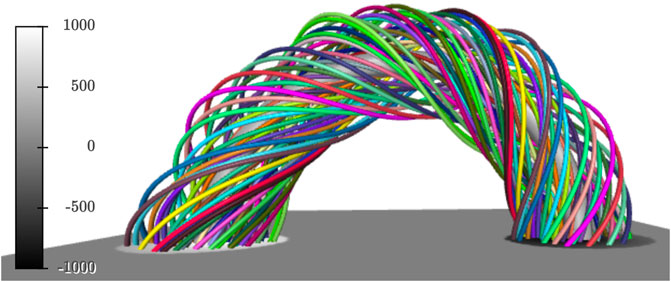
FIGURE 2. Output from the first visualisation of the flux rope. The axis is shown by a thicker grey line while the other field lines are shown by randomly coloured thinner lines. B_z from the lower boundary of the domain is also shown.

2.2.3 Computing T_g

When the axis coordinates are confirmed, the corresponding unit tangent vectors $(\widehat{T})$ are first computed. These are then used in a loop through each field line to find the unit normal vector from each point along the axis to a point on the chosen field line using the find_V function. For this step, the field lines are traced at a higher resolution than the axis to provide a greater search interval. For a given axis coordinate, unit vectors are computed to a range of field line coordinates. The pairing with the dot product closest to 0 is then taken as the sought-after normal vector and the process repeats for the next axis coordinate. To minimise mistaken matches in complex cases it is required that the rotation angle between consecutive unit normal vectors does not exceed a given value. Additionally, when all axis coordinates have been matched with a field line coordinate, the inner 80% (i.e., excluding 10% from each footpoint) of the paired unit tangent vectors and unit normal vectors are tested to ensure their dot products do not exceed 0.01. Where this occurs, the unit vector normals for the entire field line are returned as NaN because it indicates that the field line may not belong to the FR or potentially bad search parameters.

When the unit normals have been computed for each field line in the FR, the distance along the axis is calculated using the calc_s function. The calc_dVds function is then used to perform simple differencing to evaluate the latter part of Eq. 1, namely, $\frac{d\widehat{\mathbf{V}}(s)}{ds}$. The cross product of this with the unit vector normals is then computed. Finally the dot product of that result with the unit tangent normal is computed and all multiplied by ds/2π for each point along the axis for each field line. The value for each step is saved as Tg_comps, i.e., the contribution to the T_g integral for each axis coordinate, and they are summed to return the final value of T_g for the field line.

2.2.4 Visualisation

The visualisation notebook reads the file generated by the computation notebook (stored in the Numpy npz format) and first allows the user to produce plots of T_g and T_w (Figure 3) for the FR coordinates and 2D plane selected for the axis determination (Section 2.2.2). Secondly, the user can visualise the FR and its axis. This is also done in the computation notebook, but is repeated here as a form of validation that the file was read in correctly, and for creating plots without having to redo the computation steps. Finally, it provides a visualisation of the FR whereby each segment of the field lines are coloured based on their local contribution to the total T_g integral for that field line, which illustrates how T_g is locally distributed along the field line (Figure 4). The two field line plots can be generated for all field lines intersecting the chosen plane or for the field lines from the plane that satisfy a T_g threshold.

FIGURE 3

FIGURE 3. Output from the visualisation notebook showing the T_g (A) and T_w (B) planes with their corresponding contours overlaid. A lime dot indicates the centre chosen in Figure 1. The dot is slightly displaced due to the difference in resolution.

FIGURE 4

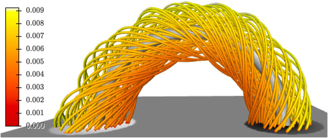
FIGURE 4. Output from the visualisation notebook. The axis is shown by a thicker grey line while the other field lines are shown by thinner lines coloured based on their local contribution to the total T_g integral. B_z at the lower boundary of the domain is also shown.

3 Discussion

We have presented a tool to investigate one of the most critical flux rope parameters, the magnetic twist, using the geometrically dependent T_g quantity and a suite of advanced visualisations such as the local contribution plot (Figure 4) which enables users to see how twist is distributed along the field lines of their flux ropes. The present workflow is liable to exclude part of the FR structure because T_w is initially used to define which field lines belong to the FR for the purposes of computing T_g. This means the Notebook provided is more suited to studying the distribution of the twist instead of FR identification. However, the user is free to select points in other ways instead of rigidly following the Notebook as written. In future versions we will implement alternative examples and provide them as Notebooks.

A current limitation for MAFIAT is that it is not suitable for low-lying FRs where field lines make multiple crossings through the photosphere because the field lines are traced to the photosphere at each end. Furthermore, for T_g in particular, FRs that are inclined at their footpoints may yield underestimations for T_g if it is not possible to find a unit normal from the axis to the target field line without going below the photosphere. Improved field line tracing and local interpolation are under development for future versions to handle these situations, which will ensure the found unit normals are more robustly computed and reduce the dependency of accuracy on field line resolution.

Presently all computations are serial. However, given that the computation of T_g is independent for each field line, they are able to be computed simultaneously. This will be addressed in a future version to improve performance. Furthermore, we plan to implement additional visualisation features such as a framework for the simple selection and investigation of individual field lines in the FR. These, and other features, highlight the fact that MAFIAT will remain under active development, with a number of improvements planned over the coming year.

Data availability statement

The datasets presented in this study can be found in online repositories. The names of the repository/repositories and accession number(s) can be found in the article.

Author contributions

DP developed the MAFIAT software with contributions from JP. All authors contributed to manuscript preparation and revision, and read and approved the submitted version.

Funding

This project has received funding from the European Research Council (ERC) under the European Union’s Horizon 2020 research and innovation programme under grant agreement No. 724391 (SolMAG) and 101004159 (SERPENTINE). The work leading to these results has been carried out in the Finnish Centre of Excellence in Research of Sustainable Space (Academy of Finland grant number 336807). JP acknowledges the Academy of Finland Project 343581 (SWATCH).

Acknowledgments

This research has made use of NASA’s Astrophysics Data System.

Conflict of interest

The authors declare that the research was conducted in the absence of any commercial or financial relationships that could be construed as a potential conflict of interest.

Publisher’s note

All claims expressed in this article are solely those of the authors and do not necessarily represent those of their affiliated organizations, or those of the publisher, the editors and the reviewers. Any product that may be evaluated in this article, or claim that may be made by its manufacturer, is not guaranteed or endorsed by the publisher.

References

Amari, T., Canou, A., Aly, J.-J., Delyon, F., and Alauzet, F. (2018). Magnetic cage and rope as the key for solar eruptions. Nature 554, 211–215. doi:10.1038/nature24671

PubMed Abstract | CrossRef Full Text | Google Scholar

Berger, M. A., and Prior, C. (2006). The writhe of open and closed curves. J. Phys. A Math. Gen. 39, 8321–8348. doi:10.1088/0305-4470/39/26/005

CrossRef Full Text | Google Scholar

Chen, J. (2017). Physics of erupting solar flux ropes: Coronal mass ejections (CMEs)—Recent advances in theory and observation. Phys. Plasmas 24, 090501. doi:10.1063/1.4993929

CrossRef Full Text | Google Scholar

Eastwood, J. P., Biffis, E., Hapgood, M. A., Green, L., Bisi, M. M., Bentley, R. D., et al. (2017). The economic impact of space weather: Where do we stand? Risk Anal. 37, 206–218. doi:10.1111/risa.12765

PubMed Abstract | CrossRef Full Text | Google Scholar

Inoue, S., Kusano, K., Büchner, J., and Skála, J. (2018). Formation and dynamics of a solar eruptive flux tube. Nat. Commun. 9, 174. doi:10.1038/s41467-017-02616-8

PubMed Abstract | CrossRef Full Text | Google Scholar

Inoue, S., Kusano, K., Magara, T., Shiota, D., and Yamamoto, T. T. (2011). Twist and connectivity of magnetic field lines in the solar active region. Astrophys. J. 738, 161. doi:10.1088/0004-637X/738/2/161

CrossRef Full Text | Google Scholar

Kilpua, E. K. J., Lugaz, N., Mays, M. L., and Temmer, M. (2019). Forecasting the structure and orientation of earthbound coronal mass ejections. Space weather. 17, 498–526. doi:10.1029/2018SW001944

CrossRef Full Text | Google Scholar

Kilpua, E., Koskinen, H. E. J., and Pulkkinen, T. I. (2017). Coronal mass ejections and their sheath regions in interplanetary space. Living Rev. Sol. Phys. 14, 5. doi:10.1007/s41116-017-0009-6

PubMed Abstract | CrossRef Full Text | Google Scholar

Liu, R., Kliem, B., Titov, V. S., Chen, J., Wang, Y., Wang, H., et al. (2016). Structure, stability, and evolution of magnetic flux ropes from the perspective of magnetic twist. Astrophys. J. 818, 148. doi:10.3847/0004-637X/818/2/148

CrossRef Full Text | Google Scholar

Török, T., and Kliem, B. (2003). The evolution of twisting coronal magnetic flux tubes. Astron. Astrophys. 406, 1043–1059. doi:10.1051/0004-6361:20030692

CrossRef Full Text | Google Scholar

Webb, D. F., and Howard, T. A. (2012). Coronal mass ejections: Observations. Living Rev. Sol. Phys. 9, 3. doi:10.12942/lrsp-2012-3

CrossRef Full Text | Google Scholar

Wiegelmann, T., Petrie, G. J. D., and Riley, P. (2017). Coronal magnetic field models. Space Sci. Rev. 210, 249–274. doi:10.1007/s11214-015-0178-3

CrossRef Full Text | Google Scholar

Zhong, Z., Guo, Y., and Ding, M. D. (2021). The role of non-axisymmetry of magnetic flux rope in constraining solar eruptions. Nat. Commun. 12, 2734. doi:10.1038/s41467-021-23037-8

PubMed Abstract | CrossRef Full Text | Google Scholar