 Jeff Klenzing
 Jonathon M. Smith
 Alexa J. Halford
 J. D. Huba
 Angeline G. Burrell
94% of researchers rate our articles as excellent or good
Learn more about the work of our research integrity team to safeguard the quality of each article we publish.
Find out more
TECHNOLOGY AND CODE article
Front. Astron. Space Sci., 02 December 2022
Sec. Space Physics
Volume 9 - 2022 | https://doi.org/10.3389/fspas.2022.1066480
This article is part of the Research TopicSnakes on a Spaceship—An Overview of Python in Space PhysicsView all 31 articles
sami2py is a Python module that runs the SAMI2 (Sami2 is Another Model of the Ionosphere) ionospheric model, as well as load and archive the results. SAMI2 is a model developed by the Naval Research Laboratory to simulate the motions of plasma in a two-dimensional ionospheric environment along a dipole magnetic field. SAMI2 solves for the chemical and dynamical evolution of seven ion species in this environment (H+, He+, N+, O+,
SAMI2 is a model developed at the Naval Research Laboratory to simulate the motions of plasma in a two dimensional (2D) ionospheric environment along dipole magnetic field lines (Huba et al., 2000). The model itself is written in FORTRAN (Backus and Heising, 1964) and distributed under an open source license. It has been applied to a variety of low-latitude ionospheric physics problems, including longitudinal variation of airglow measurements (England et al., 2008), the effect of neutral winds on instability growth rates (Zhan and Rodrigues., 2018), and plasma bubble refilling rates (Otsuka et al., 2021). Because of the open source nature of the code, other variations have been built with additional physics considerations such as photoelectron transport (Varney et al., 2012; Krall and Huba, 2019).
The sami2py software package (Klenzing et al., 2022) is an interface built in Python (Van Rossum and Drake, 2009) designed to initiate, modify, and manage runs of the SAMI2 model for ionospheric studies. The original version was written in MatLab (Higham and Higham, 2016) as part of a systematic study of solar minimum (Klenzing et al., 2013), but has been rewritten and modified to comply with the Heliophysics Python ecosystem (e.g., Annex et al., 2018; Burrell et al., 2018). The software has been made open source and available to the community for modification to better improve reproducability of ionospheric research (e.g., Gil et al., 2016). Section 2 will discuss the implementation of sami2py. Section 3 will discuss a brief overview of a standard workflow of the code, including example output and plots. Section 4 will describe several ongoing applications of the sami2py project using the Application Usability Level (AUL) Framework (Halford et al., 2019). This framework was recently developed to help track the progress of a product and ensure that it will be usable by the intended user community. The framework matches the progress to similar frameworks such as the technology readiness levels used by the space hardware community and the readiness levels used by the National Oceanic and Atmospheric Administration (NOAA).
The sami2py project will be discussed in terms of the three major components: the core ionospheric solver, the component models, and the Python interface.
The core of the code is the FORTRAN ionospheric dynamics engine. At this stage of development, this is numerically unchanged from the original release of the SAMI2 model, though the handling of some variables has been updated to accommodate compilation using GNU compilers (e.g., gfortran team, 2022). SAMI2 solves for the chemical and dynamical evolution of seven ion species in this environment (H+, He+, N+, O+,
The SAMI2 model simulates the production, motion, and loss of ions along a two-dimensional slice of Earth’s ionosphere, as shown in Figure 1. This slice is aligned with magnetic field lines as calculated for an offset tilted dipole field. The continuity, momentum, and temperature equations for ions and electrons are solved. The model is initialized and driven by empirical models, as discussed in Section 2.2. A series of scaling factors can be used to alter the magnitude of these empirical values through the namelist file. In general, the model is run for 24 h before modelled values are output to files. This is done to clear transients from the system.
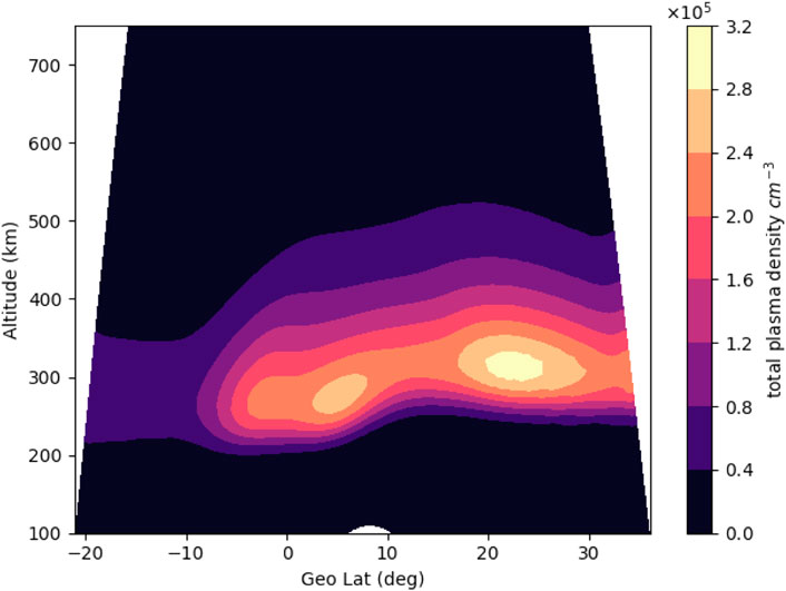
FIGURE 1. Example output of the SAMI2 model.
The sami2py software builds on the modular nature of the SAMI2 model. In the original release, SAMI2 used four key empirical models to prime the ionospheric solutions: NRLMSISe-00 (Picone, 2002) to provide the neutral atmosphere, EUVAC (Richards et al., 1994) to provide the EUV spectrum, HWM-93 to provide neutral winds (Hedin et al., 1993b,a), and the Fejer-Scherliess model of low-latitude E×B drifts (Scherliess and Fejer, 1999). sami2py updates these component models, whose acronyms are defined below, to the latest versions and includes the older versions as optional inputs. Additionally, the number of scalable parameters has been expanded. A full list of the available models and scalable parameters is included in Table 1.
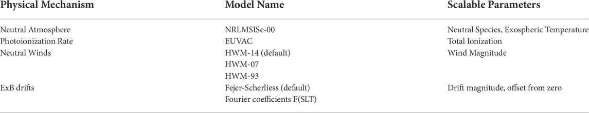
TABLE 1. Component Models in sami2py 0.3.0.
The Naval Research Laboratory Mass Spectrometer and Incoherent Scatter radar (NRLMSIS) model is a semi-empirical model representing multiple decades of neutral atmospheric measurements, including mass spectrometer, radar, and satellite drag data (Picone, 2002). The version implemented in sami2py is a modification of the extended version of the model released in 2000 (NRLMSISe-00). During the solar minimum between cycles 23 and 24, record low densities in the thermosphere were observed through satellite drag measurements Emmert et al. (2010) and direct measurement of neutral pressure density (Haaser et al., 2010). These measurements were outside of the underlying database used to construct the model. Solomon et al. (2010) suggested that anomalously low Extreme Ultraviolet (EUV) radiation during this period resulted in a much cooler thermosphere than expected from the radio flux proxy for solar activity (F10.7). Since F10.7 rather than EUV is used to drive the thermospheric model, Klenzing et al. (2013) implemented a scalar factor for the exospheric temperature in their empirical study of altered electrodynamics during extreme solar minima. The SAMI2 model already allows users to scale the resultant density profiles independently for each species after NRLMSISe-00 has run. The modification implemented here adds the capability to scale the exospheric temperature directly in NRLMSISe-00 in addition to constantly scaling each species. An example of the effect of this reduced temperature run is shown in Figure 2.
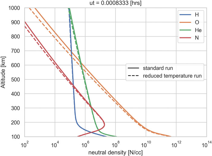
FIGURE 2. Modification of the NRLMSISe exospheric temperature.
The Extreme Ultraviolet for Aeronomic Calculations (EUVAC) model provides a calculation of the EUV flux as a function of the solar radio flux proxy F10.7 (Richards et al., 1994). For SAMI2, the model is used to calculate the photo-ionization rate of the ionosphere. While the implementation is unchanged from the SAMI2 1.00 release, a scalar parameter has been added to the code to allow sensitivity studies for directly changing the total photo-ionization rate.
The Horizontal Wind Model (HWM) provides a statistical view of neutral winds gathered from world-wide Fabry-Perot Interferometers, Incoherent Scatter Radars, satellites, and rockets (Drob et al., 2015). The latest version (HWM14) is incorporated as the default, thought users can run numerical experiments with HWM07 (Drob et al., 2008) and HWM93 as options.
The Fejer-Scherliess model of E×B drift climatology (e.g., Scherliess and Fejer, 1999) provides the two-dimensional drifts perpendicular to the magnetic field lines as a function of local time, solar activity, day of year, and longitude. This is done through cubic spline fits to data from the Jicamarca Incoherent Scatter Radar and the Atmospheric Explorer E satellite. The model is unchanged in the sami2py implementation. As in SAMI2, scalar parameters allow users to directly change the magnitude and offset of the drifts.
An alternative E×B is provided for users wanting to investigate alternate drift climatologies. Since the model is constrained to a local series of flow tubes in a single magnetic meridian, the alternate model is incorporated as a series of Fourier coefficients that are user-specified that describe a function of Solar Local Time (SLT), as shown in Eq. 1.
This allows users with direct measurements to create a localized drift model. Examples of this type of usage are presented in Klenzing et al. (2013) and Smith and Klenzing (2022). An additional input file to the FORTRAN code names exb.inp was added so that the localized model can be changed without recompiling the FORTRAN engine. Note that this creates a function that averages to zero over all local times, ensuring that there is no net upward or downward drift over the course of a day.
The sami2py Python code wraps the compiled SAMI2 FORTRAN engine (see Figure 3) in a standardized Python package. It provides an interface for users to directly update the namelist and E×B input files via keywords, and returns the results in an xarray.Dataset object (Hoyer and Hamman, 2017).
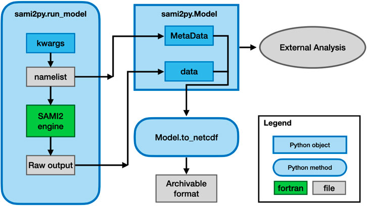
FIGURE 3. Block diagram of the sami2py workflow.
The core SAMI2 code in sami2py is compatible with FORTRAN 90 and is suitable for compilation under multiple compilers. The variable parameters, such as geographic location, solar activity, and season, are input via a namelist file, and the resulting modelled parameters are sent to binary output files. An additional exb.inp file is included to generate alternate E×B drift models via a Fourier series over solar local time. The sami2py code provides a user interface to both the input namelist files (through the sami2py.run_model method) and the output binaries (through the sami2py.Model class).
The method sami2py.run_model allows the user to directly run the compiled FORTRAN executable. The namelist that specifies the parameters of the model run can be adjusted via keyword arguments, which are fully documented in the code docstrings and in the detailed documentation that is available in the GitHub repository and online at readthedocs. This includes a user-specified “tag” to quickly describe the run for archival purposes (e.g., “solarmin”). The FORTRAN executable saves each variable as a separate file. By default, this method will move all of the output files, as well as the input namelist and exb.inp files, to an archival directory. All files are grouped under subdirectories by the tag name, longitude, and date in case a user runs multiple dates or locations for the same input conditions.
The sami2py.Model class loads the raw output of the model run. It loads each individual file and reshapes them into a single xarray. Dataset object for convenience of use. This class will also load the namelist info as metadata to allow inspection of input parameters, as well as any custom E×B input that was used. When working within sami2py, this information is stored in the model.MetaData object as a dictionary. The parameters are reshaped as 4D arrays with appropriate coordinates. Examples are shown in the sample code in Section 3. Users may run analysis directly from the Model object or save to a single file.
For portability and reproducability, both data and metadata can be exported to a netCDF4 file (Whitaker et al., 2020) using the to_netcdf method on the model. The metadata will be included as top-level attributes in the output file, documenting how the run was initialized and including both the sami2py version number and commit hash (in case a custom branch based on an official version was created). The netCDF4 versions of the file are constructed to be compatible with pysat.
The pysat ecosystem (Stoneback et al., 2018) has evolved to support management and analysis of a number of data sets throughout the space science community. The core pysat engine provides a framework to manage data sets, including acquisition, archival, and management. As a management tool, it has been used operationally in missions and analysis projects, including the ICON and COSMIC2 missions. A series of libraries has been written to translate between the core pysat commands and individual data sets. This standardization allows pysat to manage the metadata as well.
These files can be integrated into the pysat ecosystem by using the custom sami2py instrument module at pysatModels (Burrell et al., 2022). This package includes a number of other tools to compare observational data with models.
This section demonstrates how sami2py can be used in a research workflow to run and analyze the SAMI2 model and output.
The code here has been tested in linux, Mac, and Windows environments through Github Actions. Each environment is tested through a unit test suite with 97.6% code coverage as of version 0.3.0. The unit tests are configured to use the latest python packages under python 3.9 and 3.10 environments, as well as a version limited to numpy 1.20 under python 3.8. The specific versions used for the core requirements as of the publication of this paper are listed in Table 2.
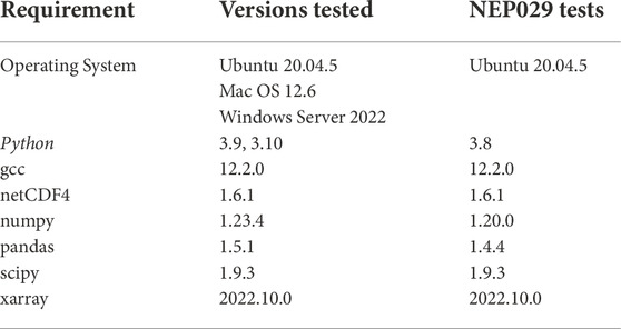
TABLE 2. Environments currently tested for sami2py 0.3.0.
The sami2py.run_model method and sami2py.Model class provide the core functionality of sami2py. The following code snippet prepares the archive directory, and specifies the time and location for the run as well as declaring custom E×B input.
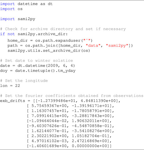
Note that setting the user archive directory only needs to be run when the package is first installed.
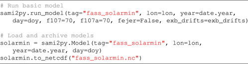
Now that the custom input has been declared and the environment is prepared for archival, the model can now be executed. The time, location, F10.7 and E×B are provided to the sami2py.run_model method. Upon completion the model output is loaded as a sami2py.Model object and archived as a netCDF file.
The following code snippet loads the archived model run, adds a new variable to the data set which consists of the total plasma density, and then plots the total plasma density as a function of local time and altitude with the E×B drift superimposed over the density. Note that by default, the ion density variable (deni) is a four-dimensional object, with one of the dimensions (retrievable as ion) specifies the individual ion species. A summation over this third axis is needed to extract total ion density.
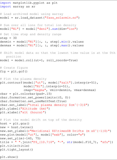
The resulting figure is shown in Figure 4.
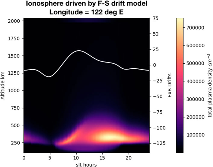
FIGURE 4. Example output ionosphere driven by custom drifts from the Fejer-Scherliess model.
The AUL framework is divided into three phases with three levels each as shown in Table 3 Halford et al. (2019). Examples of use are in the paper and a full example of the AUL framework applied to the development of a project can be found in Cid et al. (2020). The first phase focuses on basic research, the identification of the user, and agreement between the researcher and users of the intended application and requirements. The second phase develops and tests the application in a similar environment to where it will be operational. In the case of a software development such as sami2py this may include common operating systems and Python installations. The third phase includes the delivery of the application into the operational environment for routine use. The definitions of these AUL parameters are defined in the context of sami2py in Table 4.
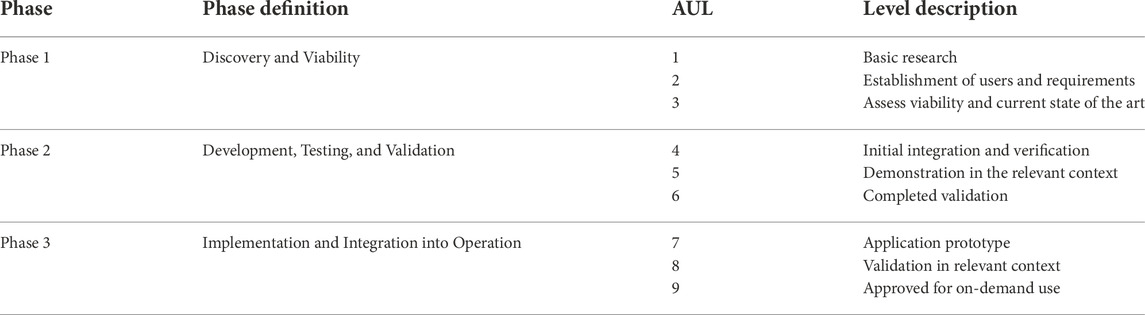
TABLE 3. A brief description of the AUL phases and levels as outlined in Halford et al. (2019).
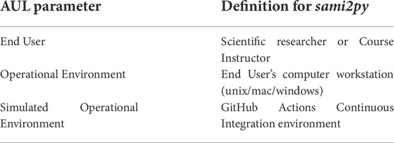
TABLE 4. AUL definitions for sami2py.
At this phase in project development, we have identified three core use cases of the software: The use of early-phase research projects to perform key sensitivity studies, as a key dependency in the growin software package (Smith and Klenzing, 2020), and as an educational tool for classes to teach ionospheric electrodynamics. We will discuss each of these individually through the framework of the AUL framework summarized in Table 3 as each as different users and requirements. The AUL framework provides a standardized scale for software and other projects on a scale of 1–9, analogous to the Technology Readiness Levels often used for flight hardware projects. The first two applications have been identified as having completed validation (AUL 6), whereas the third application (use as an educational tool) is still at an AUL 1. This section will document the steps we have taken to reach these AUL levels.
One of the applications of sami2py is for early-phase research projects. The user is the broader ionospheric research community who are communicated with on a direct basis with the development team and at conferences such as CEDAR. The operational environment is then considered to be an individual’s work computer.
An example of the early-phase research projects is running sensitivity studies on proposed physical forcing mechanisms. For this paper, an example of an identified user for this application is Klenzing et al. (2013) where the early phase research includes a series of sensitivity studies for proposed modifications to ionospheric drivers under extremely low levels of solar activity. This study was originally conducted using a prototype of the sami2py model written in MatLab, but the functionality applies to the Python version as well. Each empirical model that drives the SAMI2 ion dynamics engine can be modified to reflect proposed changes to the forcing of the ionosphere, including reductions in exospheric temperature for the MSIS model and the direct input of user-specified E×B drift profiles as a function of local time.
Examples of how the ionospheric density changes by altering the E×B drift assumptions are shown in Figures 4, 5. Each plot shows the evolution of the vertical ionospheric density profile over time. The white line plotted above the ionospheric density represents the driving E×B timeseries used in sami2py, with Figure 4 driven by the Fejer-Scherliess model (Scherliess and Fejer, 1999) and Figure 5 driven by climatology measured by the Coupled Ion-Neutral Dynamics Investigation (CINDI) mission of opportunity (Smith and Klenzing, 2022).
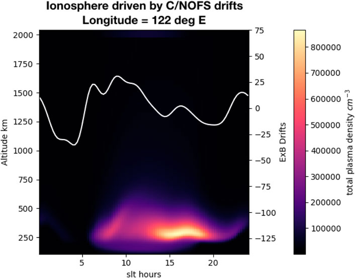
FIGURE 5. Example output ionosphere driven by custom drift climatology fit to C/NOFS data.
The work discussed above has shown how a Python version of SAMI2 will provide a path beyond the current state of the art capabilities for individual research projects. The Python interface for the SAMI2 model also provides a new capability making it easier for more researchers to access and use this model, as well as document results. Moving from a MatLab interface to an open source language improves the accessibility of the work. Incorporation of the resulting modeled data into an xarray. Dataset object improves the usability of the output. The primary requirement for this application at this phase is to ensure that this Python package is open access and works across computer operating systems. We have satisfied the milestones for AUL 3 with the release of sami2py version 0.2.0 in December 2019 (Klenzing et al., 2019).
The AUL four to six milestones require improved documentation and testing of the beta prototype of the model. Changes incorporated since version 0.2.0 include docstrings for all functions, improved Continuous Integration (CI) testing, and improved compatibility with external Python packages, including numpy, xarray, and pysat. The model undergoes continuous integration tests in the GitHub Actions environment with
AUL level 7 is the Application Prototype of the project. This requires demonstration of the prototype and dissemination of results. Both of these goals are achieved with the release of version 0.3.0 (Klenzing et al., 2022) and the publication of this paper. Improvements to the user interface and code style have been implemented in version 0.3.0 to maintain PyHC standards and improve code maintainability.
For AUL 8 and 9, a finalized project for on-demand usage needs to be released. In the context of this application for sami2py, a series of updates focusing on an improved workflow and code maintainability have been identified. These are demarcated as a future 0.4.0 release. Input from the community will be evaluated alongside these updates as the user base grows.
As an additional demonstration of the prototype, the sami2py module is a central dependency for the growin python module which was written to compute the Rayleigh-Taylor instability (RTI) growth rate. The calculation of the RTI growth rate is central to the development and growth of plumes of depleted plasma, or plasma bubbles, in the bottomside of the equatorial ionosphere. The growin module uses the sami2py module to run the SAMI2 model, archive the output, and load the output into Python data structures (Klenzing et al., 2022). Similar to the example code above, drift measurements are used to create a climatological drift profile from in-situ measurements. These drifts are then passed to sami2py and an ionosphere is simulated with the typical ionospheric indices for the corresponding time period. Subsequently the produced ionospheric plasma densities, drifts, and winds are used to compute flux-tube integrated quantities necessary to compute the RTI growth rate. These growth rates have been previously used to discuss bubble occurrence frequencies obtained from the CINDI (Smith and Klenzing, 2022) and Global Observations of the Limb and Disk (GOLD) (Martinis et al., 2021) missions.
Similar to the previous application, the broader ionospheric research community is the user and will benefit from a Python version of growin and the inclusion of sami2py within it. The feasibility, viability, and expected improvements can all be found within Smith and Klenzing (2022). Thus many of the milestones have been completed for this application through the previously discussed application in Section 4.1. As shown in Table 5, the key additional requirement here is the output of neutral atmospheric data, which is required to perform the RTI calculations. This has been added to sami2py as an optional output. As the other components growin were already within the operational/end user environment, the final AUL is now dependent on the progress of sami2py. Similar to the previous application, the usage of sami2py in the growin package is at an AUL of 7.
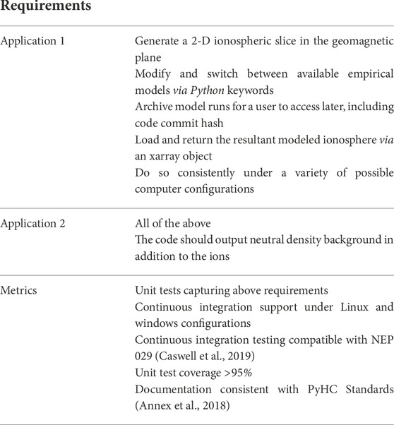
TABLE 5. Requirements and Metrics for the sami2py project.
Beyond the research community, another user community has been identified but not yet contacted. The code here can also be used as an educational tool as part of a Space Weather of Ionospheric Electrodynamics curriculum. The straightforward and modular nature of the code makes it practical to incorporate into homework or class projects as needed. As this application has been identified, but specific requirements have not been defined and incorporated into the code, this is defined as an AUL 1 project. Work is ongoing, and interested parties should contact the authors to help better refine this project and requirements for these purposes.
This work documents an overview of the sami2py code and several potential applications. The proposed applications are documented here and their progress towards on-demand use using the Application Usability Level framework. Ongoing assessment and progress of these AULs will be updated online at the projects page of the GitHub repository.
Full documentation of the code including examples is available at https://sami2py.readthedocs.io.
The data sets generated for the figures in this study can be found at zenodo: https://doi.org/10.5281/zenodo.7182786.
JK and JS wrote the Python interface to SAMI2, as well as modified the FORTRAN code. JH is the original author (with Dr. Glenn Joyce) of the FORTRAN SAMI2 code. AB contributed to overall design and interface of the code, as well as the integration into the pysat ecosystem. JK wrote the first draft of the manuscript. JS and AH wrote sections of the manuscript. All authors contributed to manuscript revision, read, and approved the submitted version.
JK and AH are supported by the Space Precipitation Impacts project at Goddard Space Flight Center through the Heliophysics Internal Science Funding Model. JS is supported by NASA NNH20ZDA001N-NASA. The research of JH was supported by NSF (AGS-1931415). AB is supported by the Office of Naval Research. This work uses the SAMI2 ionosphere model written and developed at the Naval Research Laboratory. The sami2py Python model is freely available to the community at www.github.com/sami2py/sami2py.
Author JH was employed by company Syntek Technologies Inc..
The remaining authors declare that the research was conducted in the absence of any commercial or financial relationships that could be construed as a potential conflict of interest.
All claims expressed in this article are solely those of the authors and do not necessarily represent those of their affiliated organizations, or those of the publisher, the editors and the reviewers. Any product that may be evaluated in this article, or claim that may be made by its manufacturer, is not guaranteed or endorsed by the publisher.
Annex, A., Alterman, B. L., Azari, A., Barnes, W., Bobra, M., Cecconi, B., et al. (2018). Python in heliophysics community (pyhc) standards (v1.0). Available at: https://doi.org/10.5281/zenodo.2529131
Backus, J. W., and Heising, W. P. (1964). Fortran. IEEE Trans. Electron. Comput. 13 (4), 382–385. doi:10.1109/pgec.1964.263818
Burrell, A. G., Halford, A., Klenzing, J., Stoneback, R. A., Morley, S. K., Annex, A. M., et al. (2018). Snakes on a spaceship—An overview of python in heliophysics. J. Geophys. Res. Space Phys. 123 (1210384–10), 402. doi:10.1029/2018ja025877
Burrell, A. G., Klenzing, J., and Stoneback, R. (2022). pysat/pysatModels: v0.1.0 Release (v0.1.0) Zenodo. Available at: https://doi.org/10.5281/zenodo.6567105.
Caswell, T. A., Mueller, A., Granger, B., Munk, M., Gommers, R., Haberland, M., et al. (2019). Nep 29–recommend python and numpy version support as a community policy standard. Available at: https://numpy.org/neps/nep-0029-deprecation_policy.html
Cid, C., Guerrero, A., Saiz, E., Halford, A. J., and Kellerman, A. C. (2020). Developing the ldi and lci geomagnetic indices, an example of application of the auls framework. Space weather. 18, e2019SW002171. doi:10.1029/2019sw002171
Drob, D., Emmert, J., Meriwether, J., Makela, J., Doornbos, E., Conde, M., et al. (2015). An update to the horizontal wind model (hwm): The quiet time thermosphere. Earth Space Sci. 2 (7), 301–319. doi:10.1002/2014ea000089
Drob, D. P., Emmert, J. T., Crowley, G., Picone, J. M., Shepherd, G. G., Skinner, W., et al. (2008). An empirical model of the earth’s horizontal wind fields: Hwm07. J. Geophys. Res. 113 (A12), A12304. doi:10.1029/2008ja013668
Emmert, J. T., Lean, J., and Picone, J. M. (2010). Record-low thermospheric density during the 2008 solar minimum. Geophys. Res. Lett. 37. doi:10.1029/2010gl043671
England, S. L., Immel, T. J., and Huba, J. D. (2008). Modeling the longitudinal variation in the post-sunset far-ultraviolet oi airglow using the Sami2 model. J. Geophys. Res. 113 (A1). doi:10.1029/2007ja012536
gfortran team (2022). The gnu fortran compiler. Available at: https://gcc.gnu.org/onlinedocs/gcc-12.2.0/gfortran/
Gil, Y., David, C. H., Demir, I., Essawy, B. T., Fulweiler, R. W., Goodall, J. L., et al. (2016). Toward the geoscience paper of the future: Best practices for documenting and sharing research from data to software to provenance. Earth Space Sci. 3 (10), 388–415. doi:10.1002/2015ea000136
Haaser, R. A., Earle, G. D., Heelis, R. A., Coley, W. R., and Klenzing, J. H. (2010). Low-latitude measurements of neutral thermospheric helium dominance near 400 km during extreme solar minimum. J. Geophys. Res. 115 (11), 1–5. doi:10.1029/2010ja015325
Halford, A. J., Kellerman, A. C., Garcia-Sage, K., Klenzing, J., Carter, B. A., McGranaghan, R. M., et al. (2019). Application usability levels: A framework for tracking project product progress. J. Space Weather Space Clim. 9, A34. doi:10.1051/swsc/2019030
Hedin, A. E., Fleming, E. L., Manson, A. H., Schmidlin, F. J., Avery, S. K., Clark, R. R., et al. (1993a). Empirical wind model for the middle and lower atmosphere – part 2: Local time variations.” in NASA technical memorandum 104592. Greenbelt, MD, United States: NASA. Available at: https://ntrs.nasa.gov/citations/19940017389
Hedin, A. E., Schmidlin, F. J., Fleming, E. L., Avery, S. K., Manson, A. H., and Franke, S. J. (1993b). NASA technical memorandum 104581. Greenbelt, MD, United States: NASA. Empirical wind model for the middle and lower atmosphere – part 1: Local time average. Available at: https://ntrs.nasa.gov/citations/19930015971
Higham, D. J., and Higham, N. J. (2016). MATLAB guide, Vol. 150. Philadelphia, PA, United States: Society for Industrial and Applied Mathematics.
Hoyer, S., and Hamman, J. (2017). xarray: N-d labeled arrays and datasets in python. J. Open Res. Softw. 5, 10. doi:10.5334/jors.148
Huba, J. (2003). A tutorial on hall magnetohydrodynamics. Space Plasma Simulation. Lecture Notes in Physics, Vol. 615. Heidelberg: Springer. https://doi.org/10.1007/3-540-36530-3_9
Huba, J. D., Joyce, G., and Fedder, J. A. (2000). Sami2 is another model of the ionosphere (Sami2): A new low-latitude ionosphere model. J. Geophys. Res. 105 (A10), 23035–23053. doi:10.1029/2000ja000035
Klenzing, J., Burrell, A. G., Heelis, R. A., Huba, J. D., Pfaff, R. F., and Simões, F. (2013). Exploring the role of ionospheric drivers during the extreme solar minimum of 2008. Ann. Geophys. 31 (12), 2147–2156. doi:10.5194/angeo-31-2147-2013
Klenzing, J., Smith, J., and Hirsch, M. (2019). sami2py/sami2py: Version 0.2.0 – Support for xarray (v0.2.0). Zenodo. https://doi.org/10.5281/zenodo.3581453
Klenzing, J., Smith, J. M., Burrell, A. G., Kitano, R., and Hirsch, M. (2022). sami2py/sami2py: v0.3.0 (v0.3.0). Zenodo. https://doi.org/10.5281/zenodo.7277517
Klenzing, J., Smith, J. M., Kitano, R., Hirsch, M., and Burrell, A. G., (2021). sami2py/sami2py: Version 0.2.5 (v0.2.5). Zenodo. https://doi.org/10.5281/zenodo.5575825
Krall, J., and Huba, J. D. (2019). Simulation of counterstreaming h+ outflows during plasmasphere refilling. Geophys. Res. Lett. 46 (6), 3052–3060. doi:10.1029/2019gl082130
Martinis, C., Daniell, R., Eastes, R., Norrell, J., Smith, J., Klenzing, J., et al. (2021). Longitudinal variation of post-sunset plasma depletions from the global-scale observations of the limb and disk (gold) mission. JGR. Space Phys. 6 (2), 1–10. doi:10.1029/2020ja028510
Otsuka, Y., Shinbori, A., Sori, T., Tsugawa, T., Nishioka, M., and Huba, J. D. (2021). Plasma depletions lasting into daytime during the recovery phase of a geomagnetic storm in may 2017: Analysis and simulation of gps total electron content observations. Earth Planet. Phys. 5 (5), 1–8. doi:10.26464/epp2021046
Picone, J. M., Hedin, A. E., Drob, D. P., and Aikin, A. C. (2002). NRLMSISE-00 empirical model of the atmosphere: Statistical comparisons and scientific issues. J. Geophys. Res. 107 (A12), SIA 15-21–SIA 15-16. SIA 15–16. doi:10.1029/2002ja009430
Richards, P., Fennelly, J. A., and Torr, D. G. (1994). Euvac - a solar euv flux model for aeronomic calculations. J. Geophys. Res. 99 (A5), 8981–8992. doi:10.1029/94ja00518
Scherliess, L., and Fejer, B. G. (1999). Radar and satellite global equatorial f region vertical drift model. J. Geophys. Res. 104 (A4), 6829–6842. doi:10.1029/1999ja900025
Smith, J., and Klenzing, J. (2020). JonathonMSmith/growin: Beta (0.1-beta.1) Zenodo. https://doi.org/10.5281/zenodo.3678866
Smith, J. M., and Klenzing, J. (2022). Growin: Modeling ionospheric instability growth rates. J. Space Weather Space Clim. 12, 26. doi:10.1051/swsc/2022021
Solomon, S. C., Woods, T. N., Didkovsky, L. V., Emmert, J. T., and Qian, L. (2010). Anomalously low solar extreme-ultraviolet irradiance and thermospheric density during solar minimum. Geophys. Res. Lett. 37 (16), 1–5. doi:10.1029/2010gl044468
Stoneback, R. A., Burrell, A. G., Klenzing, J., and Depew, M. D. (2018). Pysat: Python satellite data analysis toolkit. JGR. Space Phys. 123 (6), 5271–5283. doi:10.1029/2018ja025297
Varney, R. H., Swartz, W. E., Hysell, D. L., and Huba, J. D. (2012). Sami2-pe: A model of the ionosphere including multistream interhemispheric photoelectron transport. J. Geophys. Res. 117 (A6), 7280. doi:10.1029/2011ja017280
Whitaker, J., Khrulev, C., Huard, D., Paulik, C., Hoyer, S., FilipePastewka, L., et al. (2020). Unidata/netcdf4-python: version 1.5.5 release (v1.5.5rel2) Zenodo. https://doi.org/10.5281/zenodo.4308773
Keywords: ionosphere, ionospheric model, SAMI2 model, python (programming language), open source software, software, plasma instability
Citation: Klenzing J, Smith JM, Halford AJ, Huba JD and Burrell AG (2022) sami2py—Overview and applications. Front. Astron. Space Sci. 9:1066480. doi: 10.3389/fspas.2022.1066480
Received: 10 October 2022; Accepted: 04 November 2022;
Published: 02 December 2022.
Edited by:
Guozhu Li, Institute of Geology and Geophysics (CAS), ChinaReviewed by:
Zhipeng Ren, Institute of Geology and Geophysics (CAS), ChinaCopyright © 2022 Klenzing, Smith, Halford, Huba and Burrell. This is an open-access article distributed under the terms of the Creative Commons Attribution License (CC BY). The use, distribution or reproduction in other forums is permitted, provided the original author(s) and the copyright owner(s) are credited and that the original publication in this journal is cited, in accordance with accepted academic practice. No use, distribution or reproduction is permitted which does not comply with these terms.
*Correspondence: Jeff Klenzing, amVmZi5rbGVuemluZ0BuYXNhLmdvdg==
†These authors have contributed equally to this work and share first authorship
Disclaimer: All claims expressed in this article are solely those of the authors and do not necessarily represent those of their affiliated organizations, or those of the publisher, the editors and the reviewers. Any product that may be evaluated in this article or claim that may be made by its manufacturer is not guaranteed or endorsed by the publisher.
Research integrity at Frontiers
Learn more about the work of our research integrity team to safeguard the quality of each article we publish.