Using MEPED observations to infer plasma density and chorus intensity in the radiation belts

Efforts to model and predict energetic electron fluxes in the radiation belts are highly sensitive to local wave-particle interactions. In this study, we use multi-point measurements of precipitating and trapped electron fluxes to investigate the dynamic variation of chorus wave-particle interactions during the 17 March 2013 storm. Quasilinear theory characterizes the chorus wave-particle interaction as a diffusive process, with the diffusion coefficients depending on the particle energy and pitch angle, as well as the background plasma parameters such as the wave intensity and plasma density. These plasma parameters in the radiation belts are spatially localized and time-varying, so we construct event-specific diffusion coefficients using MEPED (onboard POES/MetOp) measurements of electron fluxes at low Earth orbit. This new method provides realistic diffusion coefficients for chorus waves that account for changes in the wave intensity, the plasma density, and the magnetic field strength in the outer radiation belt. We show that the inferred chorus intensity is significantly lower than previous estimates that use MEPED observations since the same amount of increased precipitation by 30–300 keV electrons can be explained by a change in the plasma density. This technique therefore allows for us to create time varying, global maps of the plasma-gyrofrequency ratio (fpe/fce), and therefore plasma density, in the outer radiation belts using the MEPED measurements. The global density estimates compare reasonably well to in situ density measurements from RBSP-B.

1 Introduction

The Earth’s radiation belts are composed of highly energetic electrons and ions that interact with the colder, denser background plasma. This collocation of the dense background plasma and the radiation belts creates a natural laboratory for studying wave-particle interactions in a plasma. The cold plasma generates several types of waves, including whistler-mode chorus waves driven by an electron temperature anisotropy. The higher energy radiation belt particles play no role in the generation of chorus waves, but they strongly interact with the waves through collisionless Landau and cyclotron damping. This wave-particle interaction can pitch angle scatter electrons near the resonant energy, causing them to precipitate into the ionosphere where they can drive the aurora (e.g., Abel and Thorne, 1998).

In this study, we are interested in calculating event-specific chorus diffusion coefficients for later use in the K2 modeling framework. K2 models the time evolution of electron phase-space density using test particles in MHD fields (Elkington et al. 2002, 2004). This MHD-test particle method allows for accurate modeling of both global effects such as radial transport and magnetopause shadowing (Elkington et al., 1999, 2003; Fei et al., 2006), as well as local wave-particle interactions such as quasilinear diffusion due to chorus waves modeled by a 2D Stochastic Differential Equation (Tao et al., 2008; Zheng et al., 2014). The wave-particle interaction is strongly determined by the wave properties in the radiation belts, and in this paper we develop a novel method for estimating these wave properties on a dynamic, global scale.

In the radiation belts, the colder background plasma is typically anisotropic with a higher temperature in the direction perpendicular to Earth’s magnetic field. Electron populations with this temperature anisotropy drive an instability that produces whistler-mode chorus waves, while anisotropic ion populations produce electromagnetic ion-cylotron (EMIC) waves (Kennel and Petschek, 1966; Omura et al., 2009). The whistler-mode chorus waves interact strongly with relativistic electrons and are the focus of this current study due to the ability to measure their precipitation into the ionosphere using the MEPED instrument on the POES and MetOp spacecrafts. EMIC waves are also important for the diffusion and loss of highly energetic electrons (>4 MeV) (Ross et al., 2020, 2021) and will be the subject of future studies.

Since the energetic electrons have no role in generating chorus waves, the wave-particle interaction is best described through the diffusion equation obtained by quasilinear theory. Quasilinear theory is a modification to typical linear solutions of the Boltzmann equation, where a slow time dependence is included for the zeroth order terms. In effect, this allows the Boltzmann equation to be solved for the case where the initial electron distribution is changing in time due to the wave losing energy to the electrons through Landau and cyclotron damping. This solution results in a standard diffusion equation, with the diffusion coefficients depending on the wave properties (Lyons and Williams, 1984).

To model the diffusion process accurately and efficiently, we need to specify a priori the properties of the chorus waves in the radiation belts. This is traditionally done through assembling statistical maps of the wave intensity ${\left|{\mathrm{B}}_{\mathrm{w}}\right|}^2$, wave frequency distribution, and the plasma frequency to gyrofrequency ratio ${\mathit{f}}_{\mathit{p}\mathit{e}}/{\mathit{f}}_{ce}$ (Albert et al., 2009; Horne et al., 2013). The empirical nature of these diffusion coefficients leads to an inconsistency with radiation belt modeling, which seeks to understand the dynamic evolution of electron fluxes during strong geomagnetic storms where intense chorus waves are not expected to strictly follow statistical patterns. Recently, Li et al. (2013) and Ni et al. (2014) developed a method to use MEPED measurements to infer the chorus intensity as a function of location and time during a geomagnetic storm. This method was used to create a set of event-specific diffusion coefficients for chorus waves in Ma et al. (2018). In this paper we expand on this method by calculating the $f_{pe}/f_{ce}$ ratio as well as the chorus intensity. This is achieved by including an additional energy channel from MEPED and allows us to estimate the plasma density in the outer radiation belts, a critical parameter for chorus wave-particle interactions. This new method produces lower chorus intensities since the $f_{pe}/f_{ce}$ ratio strongly influences the resonant energy of the wave-particle interaction.

The remainder of this paper is organized as follows. In Section 2 the calculation of quasilinear diffusion coefficients is reviewed. The MEPED data used is provided in Section 3. In Section 4 we detail the new method for using the MEPED data to calculate event-specific chorus diffusion coefficients. Section 5 then shows the chorus intensities and plasma densities estimated from scaling the diffusion coefficients, followed by a discussion of further applications in Section 6.

2 Quasilinear diffusion coefficients

2.1 Theory overview

The Boltzmann equation plus Maxwell’s equations provide a closed set of equations to describe the kinetic behavior of a plasma. Typical solutions to this set of equations involve a perturbation approach where the velocity distribution is in the form of $f_s\left(\overrightarrow{x},\overrightarrow{v},t\right)=f_{s,0}\left(\overrightarrow{v}\right)+f_{s,1}\left(\overrightarrow{x},\overrightarrow{v},t\right)$, where $f_{s,0}\left(\overrightarrow{v}\right)$ is a zeroth order, time independent distribution (i.e., a Maxwellian or Kappa distribution), and $f_{s,1}$ is a first order plane wave fluctuation. In contrast, quasilinear theory seeks to obtain the time evolution of the zeroth order background distribution as it responds to waves with finite amplitudes (Nicholson, 1983). This is an appropriate solution for wave-particle interaction in the radiation belts as it 1) provides a time evolution of phase space density, and 2) observations show that whistler-mode chorus waves have substantial amplitudes that require nonlinear terms to be retained when solving the Boltzmann equation (Zhang et al., 2019; Malaspina et al., 2021).

The quasilinear solution to the Boltzmann equation for electromagnetic waves and relativistic particle energies is derived in Kennel and Engelmann (1966) and Lyons and Williams (1984). The solution is of the form of a diffusion equation: $\frac{\partial f_0}{\partial t}={\nabla }_{\overrightarrow{v}}\cdot \left(\overline{\mathit{D}}\cdot {\nabla }_{\overrightarrow{v}}{f}_0\right)$. Using velocity coordinates of pitch angle $\alpha =\mathrm{atan}\left(v_{\perp }/v_{\parallel }\right)$ and momentum p, and assuming azimuthal symmetry, the resulting diffusion equation is

$\begin{array}{c}\frac{\partial f_0}{\partial t}=\frac{1}{\sin \alpha }\frac{\partial }{\partial \alpha }\sin \alpha \left(D_{\alpha \alpha }\frac{\partial f_0}{\partial \alpha }+p{D}_{\alpha p}\frac{\partial f_0}{\partial p}\right)+\frac{1}{p^2}\frac{\partial }{\partial p}{p}^2\left(p{D}_{p\alpha }\frac{\partial f_0}{\partial \alpha }+p^2{D}_{pp}\frac{\partial f_0}{\partial p}\right).\end{array}(1)$

Where the diffusion coefficients are all in units of 1/s, and form the symmetric matrix

$\begin{array}{c}\overline{\mathit{D}}=\left(\begin{array}{cc}{D}_{\alpha \alpha }& D_{\alpha p}\\ D_{\alpha p}& D_{pp}\end{array}\right).\end{array}(2)$

The calculation of diffusion coefficients is detailed in Glauert and Horne (2005). In this paper we use all 4 components of the diffusion tensor in Eq. 2, however we will only show the equations for $D_{\alpha \alpha }$ for brevity. The pitch angle diffusion coefficient is

$\begin{array}{c}{D}_{\alpha \alpha }={\displaystyle \sum }_n\int dXX{D}_{\alpha \alpha }^{nX},\end{array}(3)$

where $n$ is the cyclotron harmonic, and $X=\tan \left(\varphi \right)$ with $\varphi$ as the wave normal angle. The diffusion coefficient for a given cyclotron harmonic and wave normal angle is

$\begin{array}{c}{D}_{\alpha \alpha }^{nX}=\frac{q_s^2{\omega }_i^2}{4\pi \left(1+X^2\right)N\left({\omega }_i\right)}\left(\frac{n{\mathrm{\Omega }}_s/\left(\gamma {\omega }_i\right)-{\sin }^2\alpha }{\cos \alpha }\right)\cdot B^2\left({\omega }_i\right)g\left(X\right){\left[\frac{{\left|{\mathrm{\Phi }}_{n,k}\right|}^2}{\left|v_{\parallel }-\frac{\partial \omega }{\partial k_{\parallel }}\right|}\right]}_{k_{\parallel }}\end{array}(4)$

There is an implicit summation over all of the wave modes ${\omega }_i$ that are obtained from solving the cold plasma dispersion relation (defined in Appendix A). The wave frequency distributions are often assumed to be Gaussian, such as

$\begin{array}{c}{B}^2\left(\omega \right)=A^2\exp \left(-{\left(\frac{\omega -{\omega }_m}{\delta \omega }\right)}^2\right),\end{array}(5)$

$\begin{array}{c}{A}^2=\frac{{B_w}^2}{\delta \omega }\frac{2}{\sqrt{\pi }}{\left[\mathrm{erf}\left(\frac{{\omega }_m-{\omega }_{lc}}{\delta \omega }\right)+\mathrm{erf}\left(\frac{{\omega }_{uc}-{\omega }_m}{\delta \omega }\right)\right]}^{-1}.\end{array}(6)$

The parameters ${\omega }_m$, ${\omega }_{lc}$, ${\omega }_{uc}$, and $\delta \omega$ define the Gaussian distribution, and $B_w^2$ is the peak magnetic field intensity of the chorus waves, which shows that $D_{\alpha \alpha }\propto B_w^2$. The parameters $N\left({\omega }_i\right)$ and ${\Phi }_{n,k}$ are obtained from the dispersion relation (see Glauert and Horne, 2005). Furthermore, the wavenumber is constrained by the Landau/cyclotron resonance condition

$\begin{array}{c}\omega -k_{\parallel }{v}_{\parallel }=\frac{n{\mathrm{\Omega }}_s}{\gamma }.\end{array}(7)$

The diffusion coefficient for a particle with a given pitch angle and momentum is calculated by first solving the dispersion relation in Appendix A simultaneously with Eq. 7 to obtain the resonant wave frequency and wavenumber. The unspecified parameters in Eq. 4 are then: the wave amplitude at the resonant frequency, $B^2\left({\omega }_i\right)$; the wave normal angle distribution $g\left(X\right)$; and the background plasma density $n_e$ and magnetic field $B_0$ which are also needed in solving the dispersion relation. The challenge in calculating event-specific diffusion coefficients is in specifying each of these parameters, which are sparsely measured by satellites.

The basic motion of radiation belt particles is to bounce between mirror points in each hemisphere. Along this trajectory the wave properties and background plasma will change, so the diffusion coefficients are bounce-averaged. For the pitch angle diffusion coefficient, the bounce averaging is done as (Glauert and Horne, 2005)

$\begin{array}{c}\langle D_{{\alpha }_{eq}{\alpha }_{eq}}\rangle =\frac{1}{{\tau }_B}\underset{0}{\overset{{\tau }_B}{{\displaystyle \int }}}{D}_{\alpha \alpha }{\left(\frac{\partial {\alpha }_{eq}}{\partial \alpha }\right)}^{2}dt,\end{array}(8)$

where ${\alpha }_{eq}$ is the equatorial pitch angle of the particle, and ${\tau }_B$ is the particle bounce period. The diffusion coefficients used in this paper are all bounce-averaged.

2.2 Statistical chorus diffusion coefficients

The baseline set of diffusion coefficients used in this paper are calculated using the PADIE (Pitch Angle and Energy Diffusion of Ions and Electrons) model (Glauert and Horne, 2005; Horne et al., 2013) with the procedure given in Reidy et al. (2021) and the wave dataset from Meredith et al. (2020). This set of diffusion coefficients is based on statistical aggregation of wave parameters from the DE 1, Double Star TC1, and THEMIS (A, D, E) satellites, and plasma density measurements from the CRRES satellite. The wave and plasma data used in the diffusion coefficients are binned at half integer values of L-shell, 1-hour increments of MLT, and for Kp index values of 0, 1, 2, 3, and 4+. Figure 1 shows the pitch angle, momentum, and mixed diffusion coefficients at different Kp bins for the same MLT and L-shell.

FIGURE 1

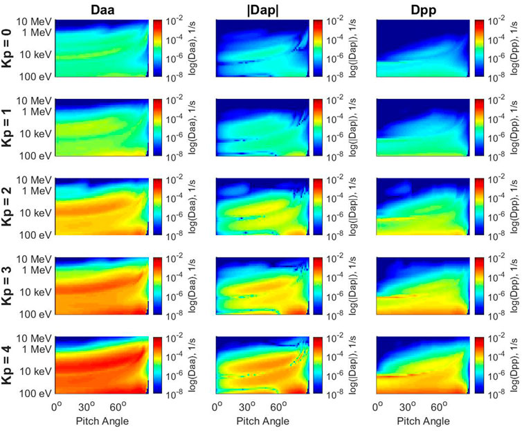
FIGURE 1. Diffusion coefficients binned by Kp index for L = 5, and MLT from 6:00 to 07:00. Note the color scale and axes are the same in each plot. The energies range from 100 eV up to 10 MeV, and the equatorial pitch angle ranges from 0.5° to 89°.

The diffusion coefficients from PADIE will be scaled with MEPED data for wave intensity, B_w, and the plasma-gyrofrequency ratio, $f_{pe}/f_{ce}$. The main benefit of using these statistical coefficients is that they use chorus frequency distributions, $B^2\left(\omega \right)$, that are fit to data (Meredith et al., 2020). The frequency distribution is still proportional to the chorus intensity, $B^2\left(\omega \right)\propto B_w^2$, but the normalization factor is computed numerically for each distribution. With this proportionality and Eqs 3, 4, the diffusion coefficients are related to the chorus intensity as

$\begin{array}{c}{D}_{\alpha \alpha }\propto B_w^2.\end{array}(9)$

This proportionality also holds for $D_{\alpha p}$ and $D_{pp}$, and is the basis for using MEPED data to scale the diffusion coefficients for event studies.

3 Medium Energy Proton and Electron Detector (MEPED) observations

Energetic electron fluxes are measured at ∼800 km altitudes using the NOAA Polar Orbiting Environmental Satellites (POES) and the European Space Agency Meteorological Observational (MetOp) satellites. The Medium Energy Proton and Electron Detector (MEPED) instrument onboard the POES and MetOp satellites measures incident electron fluxes in 4 energy channels (>30 keV, >100 keV, >300 keV, and >700 keV) with two detectors having different pointing angles. The nominal 0° detector is pointed to the spacecraft zenith, and measures electrons within the loss cone that are precipitating into the ionosphere (when at high latitudes). The nominal 90° detector is pointed behind the spacecraft’s trajectory, and measures electrons that are trapped in the radiation belts and have mirror points just below the spacecraft’s altitude. The angular width of each detector is approximately 30°, however the MEPED detectors admit fluxes through the full 180° face due to the energetic particles penetrating the shielding. This issue is discussed thoroughly in Selesnick et al. (2020), which used Monte Carlo simulations to compute accurate angular response functions for each detector. All analysis of MEPED data in this paper utilizes the angular response functions from Selesnick et al. (2020).

The construction of the MEPED instrument minimized the cross-contamination between the proton and electron channels. However, low energy protons at the right incidence angle are able to enter the electron detector where they produce a false count (Pettit et al., 2021). To account for proton contamination, we use the MEPED dataset from Pettit et al. (2019, 2021) which corrects for proton contamination by fitting the proton detector counts to obtain differential fluxes that are subtracted from the electron channels.

The POES and MetOp satellites are in polar orbit planes, providing a wide range of local time coverage. However, this coverage leaves significant gaps in the data when binning by L shell, MLT, and time. We fill these gaps in data by taking a 2-D linear interpolation in time (UT) and MLT, using the fillmissing function in MATLAB with linear interpolation. This makes the assumption that precipitation is highly localized in L shell, and therefore adjacent bins in L shell are not strongly correlated. In Figure 2 is a plot of the precipitating (0° detector) to trapped (90° detector) flux ratio on March 17-18, 2013, measured by the NOAA POES 15, 16, 17, 18, and 19 satellites, along with MetOp 1 and 2. Figure 2 shows the data filled in to create maps of precipitating/trapped flux in 1-hour local time bins, 0.5 L-shell bins. The data is later binned in 3-hour MLT increments for analysis in Section 4, however Figure 2 shows 6-hour MLT bins for space constraints.

FIGURE 2

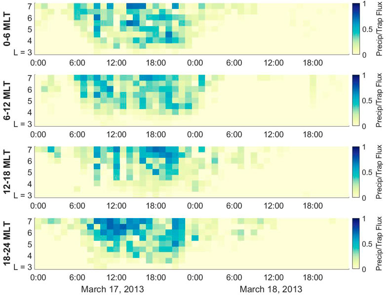
FIGURE 2. MEPED measurements of precipitating to trapped flux ratio as a function of MLT, L-shell, and universal time on March 17-18, 2013. The data are binned in 1 h time (UT) intervals and 0.5 L-shell intervals. The data are obtained from the NOAA POES 15, 16, 17, 18, and 19 satellites, along with MetOp 1 and 2.

4 Event-specific diffusion coefficients

4.1 Inferring chorus wave intensity

The method of using MEPED observations of electron fluxes in order to estimate chorus wave intensity was first developed in Li et al. (2013) and Ni et al. (2014). This method compares the observed precipitating/trapped electron flux ratio from MEPED to the ratio obtained by solving a 1-D diffusion equation in Kennel and Petschek (1966). The predicted flux inside the loss cone, corresponding to the 0-degree MEPED telescope, is (Kennel and Petschek, 1966)

$\begin{array}{c}{J}_0=\underset{E_1}{\overset{E_2}{{\displaystyle \int }}}\underset{0}{\overset{2\pi }{{\displaystyle \int }}}\underset{0}{\overset{\beta }{{\displaystyle \int }}}\frac{S\left(E\right)}{{\langle D_{\alpha \alpha }\rangle }_{LC}\cos {\alpha }_{eq}}\frac{I_0\left(\frac{{\alpha }_{eq}}{{\alpha }_{LC}}{z}_0\right)}{z_0{I}_1\left(z_0\right)}A\sin \eta d\eta d\psi d\mathit{E}.\end{array}(10)$

where I₀ and I₁ are modified Bessel functions. The corresponding flux outside the loss cone, corresponding to the 90-degree MEPED telescope, is (Kennel and Petschek, 1966)

$\begin{array}{c}{J}_{90}=\underset{E_1}{\overset{E_2}{{\displaystyle \int }}}\underset{0}{\overset{2\pi }{{\displaystyle \int }}}\underset{0}{\overset{\beta }{{\displaystyle \int }}}\frac{S\left(E\right)}{{\langle D_{\alpha \alpha }\rangle }_{LC}\cos {\alpha }_{eq}}\left[\frac{I_0\left(z_0\right)}{z_0{I}_1\left(z_0\right)}+\log \left(\frac{\sin {\alpha }_{eq}}{\sin \left({\alpha }_{LC}\right)}\right)\right]A\sin \eta d\eta d\psi d\mathit{E}.\end{array}(11)$

In both equations, ${\alpha }_{LC}$ is the loss cone angle at the equator, and the equatorial pitch angle ${\alpha }_{eq}$ of a particle is related to the local pitch angle $\alpha$ by

$\begin{array}{c}{\sin }^2{\alpha }_{eq}=\frac{B_{eq}}{B_{LEO}}{\sin }^2\alpha ,\end{array}(12)$

where $B_{LEO}$ is the magnetic field strength at the satellite’s location in low Earth orbit, nominally 800 km altitude. The parameter $z_0$ is related to ${\langle D_{aa}\rangle }_{LC}$, the bounce-averaged pitch angle diffusion coefficient evaluated at the loss cone angle:

$\begin{array}{c}{z}_0=\frac{2{\alpha }_{LC}}{\sqrt{{\tau }_B{\langle D_{\alpha \alpha }\rangle }_{LC}\cos {\alpha }_e}}\end{array}(13)$

The integrations in Eqs 10, 11 are over a finite energy range, $\left[E_1,E_2\right]$, which we will choose to correspond to the energy ranges from MEPED. The lowest energy interval from MEPED is 30–100 keV and has the highest count rates. In Section 4.2 we further develop this scaling method to account for $f_{pe}/f_{ce}$ by also examining the energy range of 100–300 keV. The function $S\left(E\right)$ is the electron energy spectrum, which we choose as the Kappa distribution used in Ni et al. (2014).

The remaining integration variables $\psi$ and $\eta$ account for the solid angle of the detector’s field of view. The azimuthal angle $\psi$, polar angle $\eta$, and detector tilt angle $\theta$ are related to the particle pitch angle $\alpha$ by the equation

$\begin{array}{c}\cos \alpha =\cos \theta \cos \eta +\sin \theta \sin \eta \cos \psi .\end{array}(14)$

The tilt angle $\theta$ is defined such that $\theta =0°$ corresponds to the 0-degree detector looking parallel to the Earth’s magnetic field, and $\theta =90°$ corresponds to the 90-degree detector looking perpendicular to the magnetic field. The tilt angle is a known quantity from the MEPED data.

Eq. 14 can be used to write the local pitch angle $\alpha$ as a function of the integration variables, $\eta$ and $\psi$, for a known detector tilt angle. The detector is axisymmetric, so $\psi$ ranges from 0 to $2\pi$. As written, Eqs 10, 11 show the integration over the polar angle $\eta$ is from 0 to $\beta$, where $\beta$ is the half-width of the detector field of view. The MEPED detectors on POES and MetOp are typically reported to have a detector half-width of $\beta =15°$. However, as discussed in Section 3, Selesnick et al. (2020) used Monte Carlo simulations to compute accurate angular response functions for each detector that accounted for energetic electrons penetrating the shielding around the instrument. In taking the polar integrals in Eqs 10, 11 we utilize the tabulated angular response functions from Selesnick et al. (2020). This is done through the substitution

$\begin{array}{c}d\eta \to R_{Sel}\left(\eta \right)d\eta ,\end{array}(15)$

where we denote $R_{Sel}\left(\eta \right)$ as the angular response function from Selesnick et al. (2020), and we now integrate across the entire polar angle range from 0° to 90°.

The Li et al. (2013) and Ni et al. (2014) method for scaling diffusion coefficients for chorus intensity is as follows:

1) Specify the statistical diffusion coefficient to scale, $\langle {\mathrm{D}}_{\alpha \alpha }\rangle$, as a function of electron energy and pitch angle.

2) Calculate the predicted ratio of precipitating to trapped flux, $J_0/J_{90}$, using Eqs 10, 11, 12, 13, 14, 15.

3) Choose a scaling factor s and recalculate $J_0/J_{90}$ using $s⟨D_{\alpha \alpha }⟩$ as the diffusion coefficient.

4) Repeat step 3 for a wide range of scaling factors to calculate the function $J_0/J_{90}\left(s\right)$.

5) Obtain the measured precipitating to trapped flux ratio from MEPED data, ${\left[\frac{J_0}{J_{90}}\right]}_{Obs}$.

6) Solve for ${\left[\frac{J_0}{J_{90}}\right]}_{Obs}=J_0/J_{90}\left(s\right)$, which provides the scaling factor $s_r$ which $\langle D_{\alpha \alpha }\rangle$ needs to be multiplied by in order to explain the observed flux ratio.

7) The scaled diffusion coefficients are then $s_r\langle D_{\alpha \alpha }\rangle$, $s_r⟨D_{\alpha p}⟩$, and $s_r⟨D_{pp}⟩$.

This method can be applied without ever knowing the chorus wave intensity used in PADIE to calculate $⟨D_{\alpha \alpha }⟩$. The inferred chorus intensity $B_w^{\left[inferred\right]}$ in the radiation belts is

$\begin{array}{c}{B}_w^{\left[inferred\right]}=\sqrt{s_r}{B}_w^{\left[input\right]},\end{array}(16)$

where $B_w^{\left[input\right]}$ is the input for PADIE, and the square root comes from the fact that $\langle D_{\alpha \alpha }\rangle \propto B_w^2$.

Figure 3 shows an example of this scaling process, with Eq. 16 used to plot $J_0/J_{90}$ as a function of chorus wave intensity instead of the abstract scaling ratio. In Figure 3 the scaling method is applied using observed flux ratios by MEPED, leading to an inferred chorus intensity of $B_w=435$ pT from the 30–100 keV band, and an inferred chorus intensity of $B_w=825$ pT from the 100–300 keV band. Since the observed fluxes are caused by the same chorus waves in the radiation belts, the scaling method should produce the same chorus intensity values. In the next section we show that scaling the diffusion coefficients for $f_{pe}/f_{ce}$ addresses this problem.

FIGURE 3

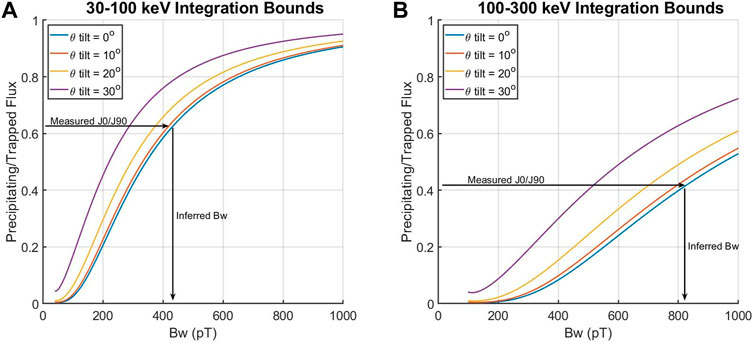
FIGURE 3. Sample calculations of the predicted ratio of precipitating to trapped flux using Eqs 10, 11, 12, 13, 14, 15, with different detector tilt angles. The inferred chorus intensity is obtained by finding where the curve for $J_0/J_{90}$ intersects the observed value by MEPED, then reading the $B_w$ value at that intersection. The black arrows show an example of this process: at 15:00 UT, 03:00 MLT, and L = 5, the measured flux ratio in the 30–100 keV band was $\frac{J_0}{J_{90}}=0.62$, which gives an inferred chorus intensity of $B_w=435$ pT from plot (A). At the same time, the measured flux ratio in the 100–300 keV band is $\frac{J_0}{J_{90}}=0.42$, so the inferred chorus intensity in plot (B) is $B_w=825$ pT. The discrepancy in the flux ratio $J_0/J_{90}$ between the two energy bands is due to chorus diffusion favoring electron energies less than 100 keV (see Figure 1). However, the inferred values of the chorus intensity should be the same for each energy band since the observed precipitation in each band is caused by the same chorus wave. This discrepancy between the inferred B_w values is the subject of Section 4.2.

4.2 Inferring plasma density

The method for scaling chorus intensity using MEPED data produces different estimates of the chorus intensity in the 30–100 keV and 100–300 keV energy ranges (Figure 3). This discrepancy was noticed in Ni et al. (2014), where they attributed the difference to 1) lower uncertainties in the measured 30–100 keV fluxes due to higher count rates, and 2) the increased importance of momentum diffusion at higher energies. We offer an alternative explanation: the diffusion coefficients assume an inaccurate plasma-gyrofrequency ratio, $f_{pe}/f_{ce}$. This section develops a method to scale diffusion coefficients with $f_{pe}/f_{ce}$, which we use to force the chorus intensity to be the same in both energy ranges.

Eqs 3, 4, 5 show how the pitch angle diffusion coefficient is calculated. The plasma-gyrofrequency ratio does not explicitly enter into those equations, but it does change the dispersion relation for chorus waves. From Appendix A, the chorus dispersion relation for parallel propagating waves ($X=\tan \psi =0$) is

$\begin{array}{c}\frac{{\omega }^2}{c^2{k}^2}={\left(1+\frac{{\mathrm{\omega }}_p^2}{{\mathrm{\Omega }}_c^2-{\omega }^2}\left(1+\frac{\left|{\mathrm{\Omega }}_c\right|}{\omega }\right)\right)}^{-1},\end{array}(17)$

which is solved simultaneously with the Landau/cyclotron resonance condition in Eq. 5. For parallel propagating waves the resonance condition yields

$\begin{array}{c}k=\frac{1}{v_{\parallel }}\left(\omega -\frac{n{\mathrm{\Omega }}_c}{\gamma }\right).\end{array}(18)$

Substituting Eq. 18 into Eq. 17, and utilizing $\gamma ={\left(1-\frac{v_{\parallel }^2}{c^2{\cos }^2\alpha }\right)}^{-1/2}$ with $\alpha$ as the pitch angle, the resonant chorus frequency $\omega$ is

$\frac{{\omega }^3}{{\mathrm{\Omega }}_c^3}\left({\gamma }^2{\sin }^2\alpha +{\cos }^2\alpha \right)+\frac{{\omega }^2}{{\mathrm{\Omega }}_c^2}\left({\gamma }^2{\sin }^2\alpha +{\cos }^2\alpha -2n\gamma \right)+\frac{\omega }{{\mathrm{\Omega }}_c}\left(n^2+\frac{{\omega }_p^2}{{\mathrm{\Omega }}_c^2}\left({\gamma }^2-1\right){\cos }^2\alpha -2n\gamma \right)+n^2=0(19)$

This is a cubic equation in $\omega /{\Omega }_c$, and the coefficients for the 0^th, 2^nd and 3^rd order terms do not depend on the plasma frequency. Therefore, the same solution for $\omega$ is obtained if ${\omega }_p$ and $\gamma$ are changed such that

$\begin{array}{c}{n}^2+\frac{{\omega }_p^2}{{\mathrm{\Omega }}_c^2}\left({\gamma }^2-1\right){\cos }^2\alpha -2n\gamma =constant.\end{array}(20)$

For parallel propagating waves only the $n=-1$ resonance is important, however we keep n in the equation since it is a constant anyways. Defining the plasma-gyrofrequency ratio as

$\begin{array}{c}R=\frac{{\omega }_p}{{\mathrm{\Omega }}_c}.\end{array}(21)$

Eq. 20 shows that two sets of parameters (subscripts 0 and 1) lead to the same solution of $\omega /{\Omega }_c$ if

$\begin{array}{c}{R}_0^2\left({\gamma }_0^2-1\right){\cos }^2{\alpha }_0-2n{\gamma }_0=R_1^2\left({\gamma }_1^2-1\right){\cos }^2{\alpha }_1-2n{\gamma }_1.\end{array}(22)$

This can be solved for ${\gamma }_1$ with the quadratic equation. However, looking at Eq. 19, we see $\gamma$ is present in the 2^nd and 3^rd order terms, and therefore changing $\gamma$ in response to ${\omega }_p/{\Omega }_c$ will change those coefficients and the overall solution for $\omega$. We therefore constrain Eq. 22 to the weakly-relativistic limit, such that $2n{\gamma }_0\approx 2n{\gamma }_1$. Then Eq. 22 simplifies to

$\begin{array}{c}{R}_0^2\left({\gamma }_0^2-1\right){\cos }^2{\alpha }_0=R_1^2\left({\gamma }_1^2-1\right){\cos }^2{\alpha }_1.\end{array}(23)$

Using $\gamma =1+E/E_r$, where $E_r$ is the electron rest mass, we express this relation in terms of particle energy,

$\begin{array}{c}{E}_1\left(E_1+2E_r\right)=E_0\left(E_0+2E_r\right)\frac{R_1^2{\cos }^2{\alpha }_1}{R_0^2{\cos }^2{\alpha }_0},\end{array}(24)$

with the quadratic solution

$\begin{array}{c}{E}_1=-E_r+\sqrt{\frac{R_0^2{\cos }^2{\alpha }_0}{R_1^2{\cos }^2{\alpha }_1}{E}_0\left(E_0+2E_r\right)+E_r^2}.\end{array}(25)$

Notice that in the nonrelativistic limit, and for ${\alpha }_1={\alpha }_0$, Eq. 24 simplifies to

$\begin{array}{c}{E}_1=E_0{\left(\frac{{\omega }_{p1}}{{\mathrm{\Omega }}_{c1}}\right)}^2{\left(\frac{{\omega }_{p0}}{{\mathrm{\Omega }}_{c0}}\right)}^{-2}.\end{array}(26)$

Eq. 25 provides an approximate relation between two different particles with different energies and plasma frequencies that yields the same solution of the dispersion relation for the chorus frequency. These two sets of particle energy and plasma-gyrofrequency parameters will therefore yield approximately the same diffusion coefficients, providing a fast and simple way of scaling $D_{\alpha \alpha }$ with changing plasma frequency. This is effectively done by setting ${\alpha }_0={\alpha }_1$, and shifting the entire diffusion coefficient $D_{\alpha \alpha }$ up or down in energy. An example of this scaling with $f_{pe}/f_{ce}$ is shown in Figure 4, where the scaling is done by shifting the whole diffusion coefficient up or down in energy based on Eq. 25.

FIGURE 4

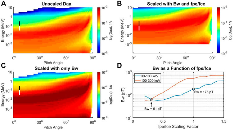
FIGURE 4. Scaling diffusion coefficients for $f_{pe}/f_{ce}$ and $B_w$. In plot (A) is the PADIE statistical diffusion coefficient $D_{\alpha \alpha }$ to be scaled. The Li et al. (2013) and Ni et al. (2014) method in Section 4.1 for scaling with ${\mathrm{B}}_{\mathrm{w}}$ is done by integrating at the loss cone from 30 to 100 keV and 100–300 keV. This integration path is shown as the thick white and black vertical lines at $\alpha \approx 7°$ in plots (A–C). Plot (D) shows the inferred value of $B_w$ as a function of scaling $f_{pe}/f_{ce}$ by a constant. The Li et al. (2013) method does not scale $f_{pe}/f_{ce}$, so it infers $B_w=175pT$, which creates the very strong diffusion coefficient in plot (C). In contrast, the new method developed in this paper finds the intersection of the curves for the 30–100 keV band and the 100–300 keV band in plot (D). This method infers $B_w=61pT$, while also scaling the diffusion coefficient up in energy using Eq. 25, with $f_{pe}/f_{ce}$ reduced by a factor of 1/3. This method produces a much weaker overall diffusion coefficient since the shift in energy puts the stronger part of the diffusion coefficient in the integration path (vertical white and black line at $\alpha \approx 7°$) when calculating $J_0/J_{90}$.

Eq. 25 gives a quick and approximate way to shift the diffusion coefficients up and down in energy when $f_{pe}/f_{ce}$ changes. We use this relation to scale the diffusion coefficients with the MEPED data by iterating over the method in Section 4.1 until the inferred $B_w$ from the 30–100 keV band matches the inferred $B_w$ from the 100–300 keV band. This is done as follows:

1) Specify the statistical diffusion coefficient to scale, $\langle D_{\alpha }\rangle$.

2) Use the method in Section 4.1 to calculate the chorus intensity in the 30–100 keV band, $B_w^{30-100}$, and the chorus intensity in the 100–300 keV band, $B_w^{100-300}$.

3) Select a range of scaling factors r for the plasma-gyrofrequency ratio.

4) Use Eq. 25 to shift the diffusion coefficient in energy, substituting $\frac{{\omega }_{p0}}{{\mathrm{\Omega }}_{c0}}=r\frac{{\omega }_{p1}}{{\mathrm{\Omega }}_{c1}}$, and ${\alpha }_0={\alpha }_1$.

5) Repeat the method in Section 4.1 to construct the curves for chorus intensity $B_w^{30-100}\left(r\right)$ and $B_w^{100-300}\left(r\right)$ as a function of the scaling factor r.

6) Find the intersection of the curves $B_w^{30-100}\left(r\right)=B_w^{100-300}\left(r\right)$. The value of $B_w$ at this intersection is the inferred $B_w$ needed to scale the diffusion coefficients, and the value of r is the factor that $f_{pe}/f_{ce}$ needs to be scaled by using Eq. 25 to scale the diffusion coefficients in energy. An example of this is shown in panel (d) of Figure 4.

5 Results

The previous section outlines two methods for scaling diffusion coefficients using observed flux ratios at low Earth orbit. The method in Section 4.1, originally developed by Li et al. (2013) and Ni et al. (2014) only uses a single energy range of 30–100 keV to infer chorus intensity, ${\mathrm{B}}_{\mathrm{w}}$. In Section 4.2 we developed a new method that utilizes measurements in both the 30–100 keV range and the 100–300 keV range to provide information to scale both ${\mathrm{B}}_{\mathrm{w}}$ and the equatorial plasma-gyrofrequency ratio, $f_{pe}/f_{ce}$. We apply both scaling methods to the statistical diffusion coefficients in Section 2.2, using the MEPED data in Section 3. Figure 5 shows examples of the original PADIE diffusion coefficients from Section 2.2, and the coefficients scaled using the methods in section 4.1 and 4.2. The coefficients scaled for both ${\mathrm{B}}_{\mathrm{w}}$ and $f_{pe}/f_{ce}$ (Section 4.2) look different than the statistical PADIE coefficients or those scaled only with $B_w$ (Section 4.1). This is because Eq. 25 shifts the whole diffusion coefficient up in energy as $f_{pe}/f_{ce}$ changes. Both sets of scaled diffusion coefficients are included in the Zenodo data repository for use in radiation belt simulations.

FIGURE 5

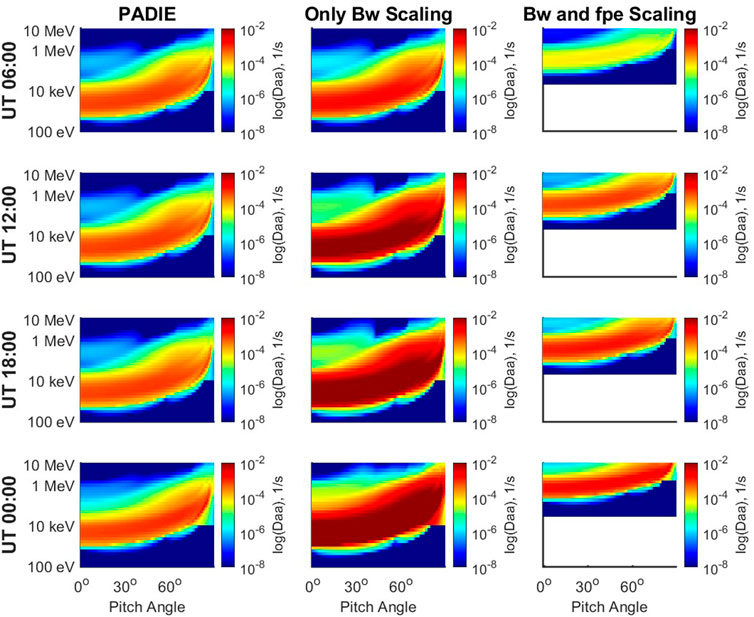
FIGURE 5. Pitch angle diffusion coefficients $D_{\alpha \alpha }$ at various times on March 17-18, 2013, for L = 6 and MLT range of 0:00-03:00. The diffusion coefficients computed from PADIE (Section 2.2) are shown in the left column and use statistical models of the plasma density and chorus intensity. The middle column shows the diffusion coefficients scaled for only the chorus intensity B_w using only the 30–100 keV energy range (Section 4.1). The right column shows the diffusion coefficients scaled for both B_w and the plasma-gyrofrequency $f_{pe}/f_{ce}$ (Section 4.2).

Figure 6 shows a snapshot of the results of scaling $D_{\alpha \alpha }$ for chorus intensity $B_w$ using the two methods. A movie showing the $B_w$ scaling for every hour of the March 17-18, 2013 event is included in the supplemental material. The method from Section 4.1 (Li et al., 2013; Ni et al., 2014) provides estimates of chorus intensity based solely on the 30–100 keV range. The new scaling method forces the inferred $B_w$ values in the 30–100 keV range to be equal to the inferred values in the 100–300 keV range by shifting the diffusion coefficient in energy. This shift in energy is due to $f_{pe}/f_{ce}$ being different in the model versus reality. By shifting the diffusion equation in energy, the stronger parts of the diffusion coefficient are moved into the integration range. In contrast, the single energy range method relies on multiplying all of $D_{\alpha \alpha }$ by a constant, and therefore large values of the precipitating/trapped flux ratio are only explained by large chorus intensities. This is reflected in the results of Figure 6, where the single energy range method consistently produces chorus intensities that are significantly higher than the chorus intensities inferred when accounting for changes in ${\mathrm{f}}_{\mathrm{p}\mathrm{e}}/{\mathrm{f}}_{\mathrm{c}\mathrm{e}}$. The ${\mathrm{B}}_{\mathrm{w}}$ only scaling in Section 4.1 is equivalent to the method developed first in Li et al. (2013). In Li et al. (2013) the inferred chorus intensity is consistently higher than the chorus intensity measured by the Van Allen Probes. Therefore, the lower estimates of chorus intensity obtained in this paper are reasonable.

FIGURE 6

FIGURE 6. Inferred values of chorus wave intensity, Bw. In plot (A) the diffusion coefficients are scaled using only the 30–100 keV range from MEPED. In plot (B) the diffusion coefficients are scaled using the new method that accounts for changes in plasma density by matching the 30–100 keV and 100–300 keV results. The inferred chorus intensity using only the 30–100 keV range (plot a) is consistently larger than the inferred chorus intensity using both energy ranges to account for changes in $f_{pe}/f_{ce}$ (plot b). A movie showing the chorus intensity at every time step is included in the supplemental materials.

The new method for scaling diffusion coefficients enables us to infer what $f_{pe}/f_{ce}$ is in the radiation belts, using only low Earth orbit measurements. Inferring $f_{pe}/f_{ce}$ on a global scale is useful for producing accurate diffusion coefficients. We can go a step further and create a global map of equatorial plasma density by assuming $f_{ce}$ is determined by a dipole magnetic field and therefore is constant in time. In Figure 7 we show the statistical density model used as an input to PADIE, and the density estimated using MEPED data and the new scaling method in Section 4.2. The supplemental materials include movies of the plasma density and $f_{pe}/f_{ce}$ ratio changing dynamically throughout the 17 March 2013 event.

FIGURE 7

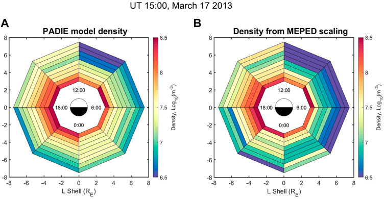
FIGURE 7. Snapshot of equatorial density. Plot (A) shows the statistical density model used to calculate diffusion coefficients with PADIE (Meredith et al., 2020). In plot (B) the inferred density is shown from the new scaling method that utilizes both the 30–100 keV and 100–300 keV energy ranges from MEPED. A movie showing the inferred density at every time step is included in the supplemental materials.

The estimated densities are compared to Van Allen Probes measurements (Kurth et al., 2015) in Figure 8. The densities are obtained from the EMFISIS instrument onboard the RBSP-B spacecraft. During the 17 March 2013 event the satellite apogee was on the nightside, and therefore sampled MLT ranges of approximately 21:00 to 04:00 when in the radiation belt (defined as L ≥ 3). Figure 9 shows the same date-model comparison but plotting the plasma-gyrofrequency ratio $f_{pe}/f_{ce}$. In Figure 10, the % error in the density is computed between the model densities and the RBSP-B measurements. The MLT and L-shell dependence of RBSP-B is shown in Figure 11. Over the 5 full passes through the radiation belts during the event, the MEPED scaling method produces density estimates that systematically underestimate the observed density but are generally close to the RBSP-B values. On three of the passes (1^st, 2^nd, and 4^th) the MEPED scaling method produces better density estimates compared to the statistical PADIE density model (Figure 10). However, on the 3^rd pass, the MEPED scaled density is not more accurate that the PADIE density model, with both models producing erratic estimates during the pass. The last pass does not produce a difference between the two models as there is no observed precipitation by MEPED at that time. The reliance on POES/MetOp observations is an inherent limitation of this method for estimating density.

FIGURE 8

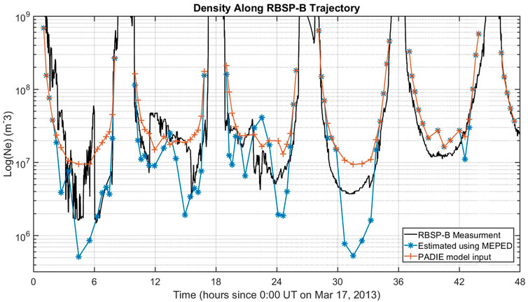
FIGURE 8. Comparison of estimated densities to Van Allen Probes measurements. The densities measured by the RBSP-B spacecraft are shown in (black), for time periods where the spacecraft was in the radiation belts (L ≥ 3). The densities estimated using the MEPED scaling method in Section 4.2 are shown in the (blue) curve, with reasonable agreement to RBSP-B. However, much of this agreement with observations is due to the high quality of the statistical density model used in the PADIE code (orange).

FIGURE 9

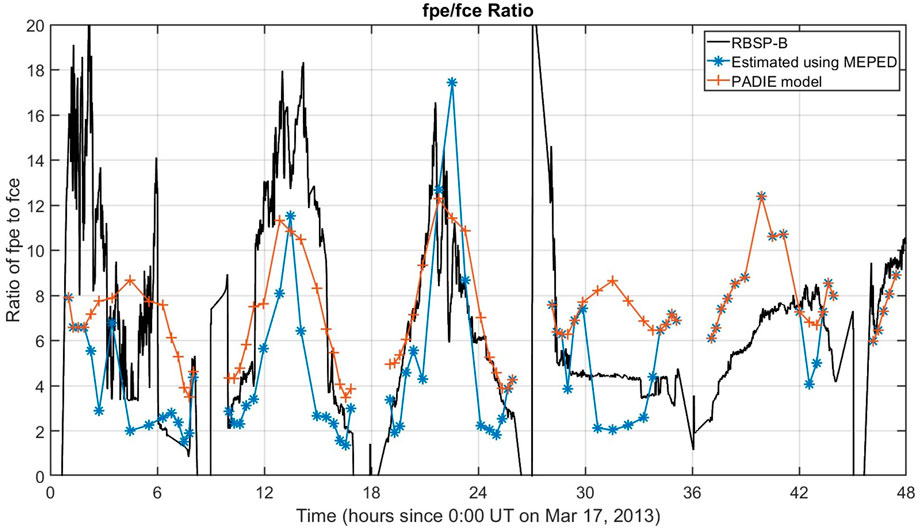
FIGURE 9. Same as Figure 8, except showing the plasma-gyrofrequency ratio $f_{pe}/f_{ce}$.

FIGURE 10

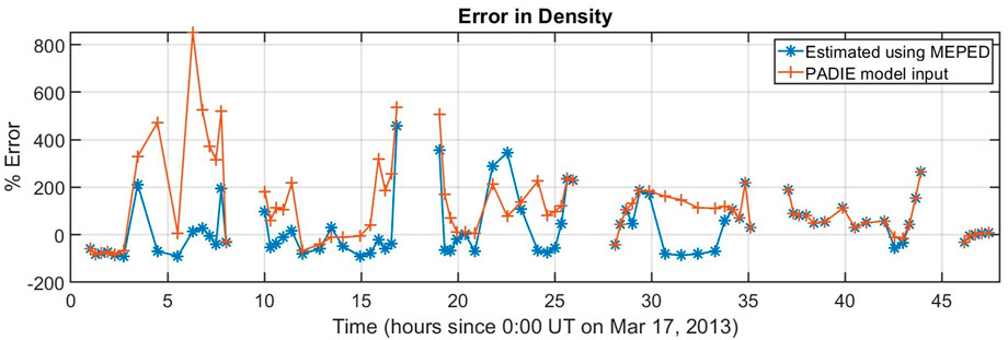
FIGURE 10. Error analysis of the density models. The percent error is computed as error = 100*(model-RBSP)/RBSP, where RBSP is the density measured by RBSP-B, and the model densities are from the MEPED scaling estimates (blue), and the PADIE statistical model (orange). By this metric, the MEPED estimated densities are typically closer to the RBSP-B measurements than the PADIE model is.

FIGURE 11

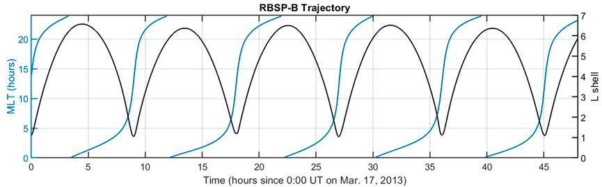
FIGURE 11. The MLT (blue) and L-shell (black) dependence of RBSP-B during the 17 March 2013 event.

6 Conclusion

Modeling wave-particle interaction in the radiation belts requires event-specific diffusion coefficients for each of the relevant waves. Whistler-mode chorus waves strongly interact with electrons in the 10 keV to 1 MeV range and will pitch angle scatter those electrons into the loss cone where they precipitate into the upper atmosphere. The MEPED instrument on the POES/MetOp spacecrafts measures the precipitating and trapped flux of electrons in this energy range, allowing the estimation of the wave parameters in the radiation belts. In this paper, we expanded the method from Li et al. (2013) and Ni et al. (2014) to estimate chorus intensity and the plasma-gyrofrequency ratio, $f_{pe}/f_{ce}$, using the MEPED observations. The estimation of $f_{pe}/f_{ce}$ creates a proxy measurement for time dependent maps of the global plasma density in the radiation belts. This new scaling method ensures the same chorus intensity is estimated using measurements in the 30–100 keV range and the 100–300 keV range. The resulting event-specific diffusion coefficients will be used in a future study with the K2 model (Elkington et al. 2002, Elkington et al. 2004).

Estimating the plasma-gyrofrequency ratio provides global, dynamic maps of the plasma density as discussed in Section 4.2. The global maps were compared to Van Allen Probes measurements of the density, showing moderately better percent errors than the statistical PADIE density model. This density estimation is not an exact process, and is limited by the following issues and approximations:

1) The scaling in Eq. 25 assumes parallel propagating chorus waves near the equator are the dominant driver of precipitating electrons measured by MEPED. The scaling equation breaks down in the relativistic limit, so care must be used to avoid scaling MeV energies down into the 30–300 keV integration range. In this paper, the diffusion coefficients needed to be scaled up in energy, so we did not encounter this issue.

2) The POES and MetOp satellites do not provide global coverage. An interpolation scheme was used to fill in spatial and temporal gaps in the data.

3) The scaling method is for the plasma-gyrofrequency ratio $f_{pe}/f_{ce}$, and changes in this ratio are attributed to changes in plasma density. In practice, this ignores non-dipolar magnetic fields which are prevalent at larger L-shells during geomagnetic storms.

4) This method only applies to time periods with enhanced chorus activity, since there needs to be enhanced electron precipitation in the 30–300 keV range. Furthermore, all precipitation in the 30–300 keV range is attributed to chorus waves and ignores all other wave modes in the radiation belts.

Furthermore, this method could be improved by skipping the energy scaling in Eq. 25 and instead using a large database of precomputed diffusion coefficients at various values of $B_w$ and $f_{pe}/f_{ce}$. A nonlinear least-squares method like the Levenberg-Marquardt algorithm can then be used to obtain the optimal solution for $B_w$ and $f_{pe}/f_{ce}$.

Data availability statement

The datasets presented in this study can be found in online repositories. The names of the repository/repositories and accession number(s) can be found below: The data, diffusion coefficients, and code used in this paper are available on Zenodo at doi: 10.5281/zenodo.7154151. The POES MEPED data is available at the National Centers for Environmental Information (NCEI) at https://www.ngdc.noaa.gov/stp/satellite/poes/dataaccess.html. The Van Allen Probes densities were obtained from the EMFISIS instrument and are available at https://emfisis.physics.uiowa.edu.

Author contributions

WL developed the methodology and analysis in this study and wrote the first draft of the manuscript. AC, AJ, and SE contributed to the conception and development of the study. JP processed the MEPED dataset. JR, SG, and RH provided the PADIE diffusion coefficients and model inputs. All authors contributed to manuscript revision, read, and approved the submitted version.

Funding

WL was supported by the NASA Living With a Star Jack Eddy Postdoctoral Fellowship Program, administered by UCAR’s Cooperative Programs for the Advancement of Earth System Science (CPAESS) under award ^#NNX16AK22G. WL, AC, AJ, and SE were supported by NASA H-SR grant ^#NNX17AI51G and NASA LWS grant ^#80NSSC21K1323. JP acknowledges funding from the NSF Coupling, Energetics and Dynamics of Atmospheric Regions, grant AGS 1651428 and the NASA Living With a Star program, grant NNX14AH54G. RH, SG, and JR were supported by NERC grant NE/V00249X/1 (Sat-Risk). RH and SG were supported by NERC National Capability grant NE/R016038/1 and NERC National Public Good activity grant NE/R016445/1.

Conflict of interest

The authors declare that the research was conducted in the absence of any commercial or financial relationships that could be construed as a potential conflict of interest.

Publisher’s note

All claims expressed in this article are solely those of the authors and do not necessarily represent those of their affiliated organizations, or those of the publisher, the editors and the reviewers. Any product that may be evaluated in this article, or claim that may be made by its manufacturer, is not guaranteed or endorsed by the publisher.

Supplementary material

The Supplementary Material for this article can be found online at: https://www.frontiersin.org/articles/10.3389/fspas.2022.1063329/full#supplementary-material

References

Abel, B., and Thorne, R. M. (1998). Electron scattering loss in earth's inner magnetosphere: 1. Dominant physical processes. J. Geophys. Res. 103 (A2), 2385–2396. doi:10.1029/97JA02919styled

CrossRef Full Text | Google Scholar

Albert, J. M., Meredith, N. P., and Horne, R. B. (2009). Three-dimensional diffusion simulation of outer radiation belt electrons during the 9 October 1990 magnetic storm. J. Geophys. Res. 114, A09214. doi:10.1029/2009JA014336styled

CrossRef Full Text | Google Scholar

Bellan, P. M. (2006). Fundamentals of plasma physics. Cambridge, UK: Cambridge University Press. doi:10.1017/CBO9780511807183styled

CrossRef Full Text | Google Scholar

Elkington, S. R., Hudson, M. K., and Chan, A. A. (1999). Acceleration of relativistic electrons via drift-resonant interaction with toroidal mode Pc-5 ULF oscillations. Geophys. Res. Lett. 26 (21), 3273–3276. doi:10.1029/1999GL003659styled

CrossRef Full Text | Google Scholar

Elkington, S. R., Hudson, M. K., and Chan, A. A. (2003). Resonant acceleration and diffusion of outer zone electrons in an asymmetric geomagnetic field. J. Geophys. Res. 108, 1116. doi:10.1029/2001ja009202styled

CrossRef Full Text | Google Scholar

Elkington, S. R., Hudson, M. K., Wiltberger, M. J., and Lyon, J. G. (2002). MHD/Particle simulations of radiation belt dynamics. J. Atmos. Sol. Terr. Phys. 64 (5-6), 607–615. doi:10.1016/S1364-6826(02)00018-4styled

CrossRef Full Text | Google Scholar

Elkington, S. R., Wiltberger, M., Chan, A. A., and Baker, D. N. (2004). Physical models of the geospace radiation environment. J. Atmos. Sol. Terr. Phys. 66, 1371–1387. doi:10.1016/j.jastp.2004.03.023styled

CrossRef Full Text | Google Scholar

Fei, Y., Chan, A. A., Elkington, S. R., and Wiltberger, M. J. (2006). Radial diffusion and MHD particle simulations of relativistic electron transport by ULF waves in the September 1998 storm. J. Geophys. Res. 111, A12209. doi:10.1029/2005JA011211styled

CrossRef Full Text | Google Scholar

Glauert, S. A., and Horne, R. B. (2005). Calculation of pitch angle and energy diffusion coefficients with the PADIE code. J. Geophys. Res. 110, A04206. doi:10.1029/2004JA010851styled

CrossRef Full Text | Google Scholar

Horne, R. B., Kersten, T., Glauert, S. A., Meredith, N. P., Boscher, D., Sicard-Piet, A., et al. (2013). A new diffusion matrix for whistler mode chorus waves. J. Geophys. Res. Space Phys. 118, 6302–6318. doi:10.1002/jgra.50594styled

CrossRef Full Text | Google Scholar

Kennel, C. F., and Engelmann, F. (1966). Velocity space diffusion from weak plasma turbulence in a magnetic field. Phys. Fluids (1994). 9, 2377–2388. doi:10.1063/1.1761629styled

CrossRef Full Text | Google Scholar

Kennel, C. F., and Petschek, H. E. (1966). Limit on stably trapped particle fluxes. J. Geophys. Res. 71 (1), 1–28. doi:10.1029/JZ071i001p00001styled

CrossRef Full Text | Google Scholar

Kurth, W. S., De Pascuale, S., Faden, J. B., Kletzing, C. A., Hospodarsky, G. B., Thaller, S., et al. (2015). Electron densities inferred from plasma wave spectra obtained by the Waves instrument on Van Allen Probes. JGR. Space Phys. 120, 904–914. doi:10.1002/2014JA020857styled

PubMed Abstract | CrossRef Full Text | Google Scholar

Li, W., Ni, B., Thorne, R. M., Bortnik, J., Green, J. C., Kletzing, C. A., et al. (2013). Constructing the global distribution of chorus wave intensity using measurements of electrons by the POES satellites and waves by the Van Allen Probes. Geophys. Res. Lett. 40, 4526–4532. doi:10.1002/grl.50920styled

CrossRef Full Text | Google Scholar

Lyons, L. R., and Williams, D. J. (1984). Quantitative aspects of magnetospheric physics. New York: Springer.styled

Google Scholar

Ma, Q., Li, W., Bortnik, J., Thorne, R. M., Chu, X., Ozeke, L. G., et al. (2018). Quantitative evaluation of radial diffusion and local acceleration processes during GEM challenge events. JGR. Space Phys. 123, 1938–1952. doi:10.1002/2017JA025114styled

CrossRef Full Text | Google Scholar

Malaspina, D. M., Jaynes, A. N., Elkington, S., Chan, A., Hospodarsky, G., and Wygant, J. (2021). Testing the organization of lower-band whistler-mode chorus wave properties by plasmapause location. JGR. Space Phys. 126, e2020JA028458. doi:10.1029/2020JA028458styled

CrossRef Full Text | Google Scholar

Meredith, N. P., Horne, R. B., Shen, X.-C., Li, W., and Bortnik, J. (2020). Global model of whistler mode chorus in the near-equatorial region (|λm|< 18°). Geophys. Res. Lett. 47, e2020GL087311. doi:10.1029/2020GL087311styled

CrossRef Full Text | Google Scholar

Ni, B., Li, W., Thorne, R. M., Bortnik, J., Green, J. C., Kletzing, C. A., et al. (2014). A novel technique to construct the global distribution of whistler mode chorus wave intensity using low-altitude POES electron data. J. Geophys. Res. Space Phys. 119, 5685–5699. doi:10.1002/2014JA019935styled

CrossRef Full Text | Google Scholar

Nicholson, D. R. (1983). Introduction to plasma theory. New York, NY: Wiley.styled

Google Scholar

Omura, Y., Hikishima, M., Katoh, Y., Summers, D., and Yagitani, S. (2009). Nonlinear mechanisms of lower-band and upper-band VLF chorus emissions in the magnetosphere. J. Geophys. Res. 114, A07217. doi:10.1029/2009JA014206styled

CrossRef Full Text | Google Scholar

Pettit, J. M., Randall, C. E., Peck, E. D., and Harvey, V. L. (2021). A new MEPED-based precipitating electron data set. J. Geophys. Res. Space Phys. 126, e2021JA029667. doi:10.1029/2021JA029667styled

PubMed Abstract | CrossRef Full Text | Google Scholar

Pettit, J. M., Randall, C. E., Peck, E. D., Marsh, D. R., van de Kamp, M., Fang, X., et al. (2019). Atmospheric effects of >30-keV energetic electron precipitation in the southern hemisphere winter during 2003. JGR. Space Phys. 124, 8138–8153. doi:10.1029/2019JA026868styled

CrossRef Full Text | Google Scholar

Reidy, J. A., Horne, R. B., Glauert, S. A., Clilverd, M. A., Meredith, N. P., Woodfield, E. E., et al. (2021). Comparing electron precipitation fluxes calculated from pitch angle diffusion coefficients to LEO satellite observations. JGR. Space Phys. 126, e2020JA028410. doi:10.1029/2020JA028410styled

CrossRef Full Text | Google Scholar

Ross, J. P. J., Glauert, S. A., Horne, R. B., Watt, C. E. J., and Meredith, N. P. (2021). On the variability of EMIC waves and the consequences for the relativistic electron radiation belt population. JGR. Space Phys. 126, e2021JA029754. doi:10.1029/2021JA029754styled

CrossRef Full Text | Google Scholar

Ross, J. P. J., Glauert, S. A., Horne, R. B., Watt, C. E., Meredith, N. P., and Woodfield, E. E. (2020). A new approach to constructing models of electron diffusion by EMIC waves in the radiation belts. Geophys. Res. Lett. 47, e2020GL088976. doi:10.1029/2020GL088976styled

CrossRef Full Text | Google Scholar

Selesnick, R. S., Tu, W., Yando, K. B., Millan, R. M., and Redmon, R. J. (2020). POES/MEPED angular response functions and the precipitating radiation belt electron flux. JGR. Space Phys. 125, e2020JA028240. doi:10.1029/2020JA028240styled

CrossRef Full Text | Google Scholar

Tao, X., Chan, A. A., Albert, J. M., and Miller, J. A. (2008). Stochastic modeling of multidimensional diffusion in the radiation belts. J. Geophys. Res. 113, A07212. doi:10.1029/2007JA012985styled

CrossRef Full Text | Google Scholar

Zhang, X.-J., Mourenas, D., Artemyev, A. V., Angelopoulos, V., Bortnik, J., Thorne, R. M., et al. (2019). Nonlinear electron interaction with intense chorus waves: Statistics of occurrence rates. Geophys. Res. Lett. 46, 7182–7190. doi:10.1029/2019GL083833styled

CrossRef Full Text | Google Scholar

Zheng, L., Chan, A. A., Albert, J. M., Elkington, S. R., Koller, J., Horne, R. B., et al. (2014). Three-dimensional stochastic modeling of radiation belts in adiabatic invariant coordinates. J. Geophys. Res. Space Phys. 119, 7615–7635. doi:10.1002/2014JA020127

CrossRef Full Text | Google Scholar

Appendix A: Whistler dispersion relation

The cold plasma dispersion relation is (Bellan, 2006):

$\begin{array}{c}\mathcal{D}\left(\omega ,k,X\right)=\left(S{X}^2+P\right){\mu }^4-\left(RL{X}^2+PS\left(2+X^2\right)\right){\mu }^2+PRL\left(1+X^2\right)\end{array}(\mathrm{A1})$

Where $\mu =ck/\omega$ is the index of refraction and $X=\tan \psi$ where $\psi$ is the wave normal angle (defined such that $\psi =0$ for waves propagating parallel to $\overrightarrow{B}$). The Stix parameters in the cold plasma dispersion relation are

$\begin{array}{c}S=1-{\displaystyle \sum }_s\frac{{\omega }_{ps}^2}{{\omega }^2-{\mathrm{\Omega }}_{cs}^2},\end{array}(\mathrm{A2})$

$\begin{array}{c}D={\displaystyle \sum }_s\frac{{\mathrm{\Omega }}_{cs}}{\omega }\frac{{\omega }_{ps}^2}{{\omega }^2-{\mathrm{\Omega }}_c^2},\end{array}(\mathrm{A3})$

$\begin{array}{c}P=1-{\displaystyle \sum }_s\frac{{\omega }_{ps}^2}{{\omega }^2},\end{array}(\mathrm{A4})$

$\begin{array}{c}R=S+D,\end{array}(\mathrm{A5})$

$\begin{array}{c}L=S-D.\end{array}(\mathrm{A6})$

The Whistler mode is obtained by solving $\mathcal{D}\left(\omega ,k,X\right)=0$ for wave frequencies at approximately ${\omega }_r\approx {\Omega }_e/2$. While oblique propagating Whistler waves ($\overrightarrow{k}$ has a component orthogonal to the background magnetic field) are important in radiation belt interactions, we will analyze the simpler case of parallel propagating waves. With $\psi =0$, and noting $2S=R+L$, the dispersion relation simplifies to

$\begin{array}{c}\mathcal{D}\left(\omega ,k,X\right)=P{\mu }^4-P\left(R+L\right){\mu }^2+PRL.\end{array}(\mathrm{A7})$

From Eq. A4, $P=0$ only occurs if ${\displaystyle \sum }_s{\omega }_{ps}^2/{\omega }^2=1$. This occurs when $\omega \approx {\omega }_{pe}$, and therefore is the Langmuir mode, so we can divide out P. Solving for ${\mu }^2$, the two solutions are

$\begin{array}{c}{\mu }^2=R,\end{array}(\mathrm{A8})$

$\begin{array}{c}{\mu }^2=L.\end{array}(\mathrm{A9})$

The Whistler mode corresponds to the R-mode solution, and Electromagnetic ion-cyclotron (EMIC) waves come from the L-mode solution, so we have

$\begin{array}{c}\frac{c^2{k}^2}{{\omega }^2}=R.\end{array}(\mathrm{A10})$

From the definitions of S and D, and ignoring ion terms,

$\begin{array}{c}R=S+D=1-\frac{{\omega }_{pe}^2}{{\omega }^2-{\Omega }_{ce}^2}\left(1-\frac{{\mathrm{\Omega }}_{ce}}{\omega }\right).\end{array}(\mathrm{A11})$

We are interested in solutions where $\omega \approx {\Omega }_c$, with the strict inequality of $\omega <\left|{\Omega }_{ce}\right|$. Therefore, we can rearrange the denominator in the second term to obtain

$\begin{array}{c}R=1+\frac{{\omega }_{pe}^2}{{\mathrm{\Omega }}_{ce}^2-{\omega }^2}\left(1+\frac{\left|{\mathrm{\Omega }}_{ce}\right|}{\omega }\right).\end{array}(\mathrm{A12})$

This shows that R is strictly positive in the Whistler regime $\left(\omega <\left|{\Omega }_{ce}\right|\right)$, and therefore Eq. A10 has real solutions.

With Eqs A10, A12, we obtain the dispersion relation for parallel propagating Whistler waves:

$\begin{array}{c}\frac{{\omega }^2}{c^2{k}^2}={\left(1+\frac{{\omega }_{pe}^2}{{\Omega }_{ce}^2-{\omega }^2}\left(1+\frac{\left|{\Omega }_{ce}\right|}{\omega }\right)\right)}^{-1}.\end{array}(\mathrm{A13})$

In Section 4.2 we use this dispersion relation along with the Landau/cyclotron resonance condition to solve for the Whistler mode frequency that is resonant with electrons at a specified energy and pitch angle.