 Chao Niu
 Yiwei Wei*
94% of researchers rate our articles as excellent or good
Learn more about the work of our research integrity team to safeguard the quality of each article we publish.
Find out more
ORIGINAL RESEARCH article
Front. Astron. Space Sci., 28 October 2022
Sec. Space Physics
Volume 9 - 2022 | https://doi.org/10.3389/fspas.2022.1061876
This article is part of the Research TopicSpace- and ground-based observations of ELF(Extremely Low Frequency)/VLF(Very Low Frequency) Electromagnetic waves and their propagation mechanismsView all 5 articles
Solar quiet variation (Sq) generated from ionospheric currents are among the most important type of geomagnetic variations. In this paper, the correlation between the geomagnetic Z component solar quiet variation (SqZ) component and the ionospheric total electron content (TEC) is discussed. For the analysis, 20 stations at middle and low latitudes are chosen, and the correlation between geomagnetic SqZ and ionospheric TEC at these stations from 2008 to 2015 is analyzed. The time delays are estimated by detecting peaks in the cross-correlation function, which shows that there is a stable correlation between SqZ and TEC. The time delay between them is largest in summer and smallest in winter, which is consistent with the Sq field intensity. With increasing latitude, the time delay decreases gradually from positive to negative, i.e., SqZ goes from being ahead of the TEC to behind it. The turning point of this change is at ca. 28°N, exactly where the Sq current vortex is located.
The geomagnetic field and ionosphere have relatively regular diurnal variations in the quiet period. The geomagnetic disturbance is often accompanied by ionospheric disturbance. When the geomagnetic field and ionosphere deviate from the normal condition seriously, it has an important influence on communication, navigation and disastrous weather prediction. The mechanism of geomagnetic disturbance and ionospheric disturbance is complex. Both the morphological analysis of small samples and the statistical analysis of large samples cannot be separated from the judgment of the sign of the beginning time and amplitude of disturbance, so the study of the relationship between geomagnetic field and ionosphere in quiet period is a basic and essential work.
Long before the existence of the ionosphere was proved, electric currents flowing in the conducting region of the upper atmosphere were predicted through observations of regular geomagnetic variations on the ground. The geomagnetic field intensity observed on the Earth’s surface is up to tens of thousands of nanoteslas, including the main contribution from the geomagnetic main field, which varies on timescales of months to billions of years (Biggin et al., 2013) and appears as the geomagnetic secular and slow variation. Other sources of the geomagnetic field—such as ionospheric currents, magnetospheric currents, etc.—contribute only a small fraction (ca. a few percent) to the total field. They are rich in frequency, varying on frequency scale of tens of hertz (geomagnetic pulsation) to 11 years (solar cycle variation). Among them, the smooth daily variations on the order of a few tens of nanoteslas on geomagnetic calm days—commonly known as solar quiet (Sq)—are generated primarily by ionospheric currents.
As the intensity and shape of the overhead current system change, the amplitude and phase of Sq change over time (Briggs, 1984; Vasyliunas, 2012). However, it is impossible to determine the pure ionospheric current system by analyzing only Sq data on the Earth’s surface. Although the Sq variation is essentially caused by ionospheric currents, secondary currents induced in the upper mantle of the Earth also contribute to it (Campbell, 1987). Besides, some researchers have found that Sq signals measured on the ground can be contaminated by the effects of magnetospheric tail currents (Olson, 1970; Xu, 1992; Olsen, 1996), the induction electric field driven by field-aligned currents of magnetospheric origin (Takeda, 2008), and conduction oceans (Kuvshinov et al., 1999; Kuvshinov and Utada, 2010). To understand Sq variation more conveniently, the equivalent Sq current system was introduced. It assumes that a two-dimensional current system flowing in a spherical thin shell (usually say at 110 km) is responsible for the Sq variations that are actually caused by three-dimensional current systems with various configurations. The equivalent Sq current system can be obtained from Sq data on the ground using a spherical-harmonic analysis technique (Yamazaki et al., 2009; Stening and Winch, 2013; Ou et al., 2017; Fujita et al., 2018). It is generally considered that the equivalent current system is horizontal and symmetric, but in some areas it may be tilted and asymmetric (Stening, 2008; Jia et al., 2017). Thus, the current-sheet assumption of Sq currents is valid only to a limited extent, and the reliability of the method for constructing the equivalent current system based on harmonic components remains to be verified by experimental data (Yamazaki and Maute, 2017; He et al., 2020). Therefore, how the ionosphere affects Sq variations is still worth studying, and a deeper understanding of geomagnetic daily variations in quiet periods is conducive to studying the ionospheric dynamo and its coupling with the atmosphere and magnetosphere. Moreover, the geomagnetic disturbance indices will be calculated more accurately, given that the quiet-day variation pattern must be removed from the magnetogram before judging the disturbance levels.
Quantitative analysis and statistical analysis of geomagnetic field and ionospheric TEC are mainly aimed at geomagnetic disturbance index and ionospheric disturbance index. In this paper, the correlation analysis is made directly by using the measured values of diurnal variation of geomagnetic field and ionospheric TEC. The study on the relationship between the variation of geomagnetic field Sq and the diurnal variation of ionospheric TEC is the breakthrough point to explore the coupling relationship between geomagnetic field and ionosphere. The geomagnetic H component is often affected by the ring current and the polar current produced by the geomagnetic disturbance, while the Z component is less affected by the geomagnetic disturbance and the solar activity, so we choose the geomagnetic Z component as the proxy of the Sq field, given that it is less sensitive to disturbances in the geomagnetic field but susceptible to changes in observation location (Takeda, 2013a). As for the ionospheric data, we use the total electron content (TEC) for analysis. First, we subject the data to some simple processing so that the cross-correlation analysis method can work. Then, the SqZ component and TEC are cross-correlated, and the spatiotemporal variation characteristics of the correlation coefficient and time delay are analyzed. Finally, we compare the present results with those of some previous studies and provide a new method for determining the position of the Sq current vortex.
The study of the correlation between the SqZ and the ionospheric TEC has important theoretical significance and practical value for accurately estimating the daily variation of the geomagnetic field Z component and the ionospheric TEC, recognizing their variation regularity and monitoring their irregular variation and violent disturbance.
The geomagnetic data were acquired from the China National Geomagnetic Network Center. We selected 10 low-latitude stations (labeled L1–L10, from 15°N to 30°N) and 10 mid-latitude stations (labeled M1–M10, from 30°N to 45°N). From L1 to L10 and from M1 to M10, their latitudes increase successively. Figure 1 shows the positions of all 20 stations, and Table 1 gives the specific time spans of the data that we used.
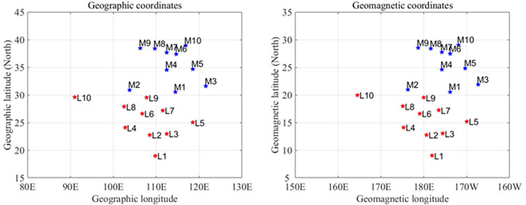
FIGURE 1. Positions of all 20 stations.
TABLE 1. Time spans of data.
The ionospheric data were derived from TEC maps from the Center for Ionospheric Analysis of the Chinese Academy of Sciences, which provides global ionosphere map (GIM) data with 15-min temporal resolution, 5° longitudinal resolution, and 2.5° latitudinal resolution.
We chose 10 International Geomagnetic Quiet Days per month from the German Geological Research Centre (GFZ Potsdam). The years 2008 and 2009 were in a solar minimum, 2010 and 2011 were in a rising phase of the solar cycle, 2012–2014 were in a solar maximum, and solar activity began to decline in 2015.
We aimed to analyze the relationship between the Z components of the geomagnetic field and the ionospheric TEC during geomagnetic quiet periods. Therefore, we pre-processed the data as follows.
1) We used cubic-spline interpolation to give the GIM data a spatial resolution of 0.5°, and then we found the grid point closest to each station. We used the TEC value of the selected grid point as the ionospheric datum of the corresponding station.
2) The 15-min mean data were obtained by averaging the geomagnetic Z component, so that the geomagnetic data could have the same temporal resolution as that of the ionospheric TEC values.
3) To reduce the impact of long-term changes and daily changes, we used the first value at local time for each day as the basic value, and subtracted it from the diurnal data. Therefore, the daily time series started from zero. The geomagnetic and ionospheric data are denoted as dqZ and dqTEC, respectively, where “d” denotes diurnal and “q” denotes quiet.
4) From these data of 10 quiet days in each month, we obtained the average Sq variation of the Z component of the geomagnetic field for each month (denoted as SqZ) and the average daily ionospheric TEC (denoted as SqTEC). Here, SqTEC refers to the TEC time series corresponding to the change of the geomagnetic Sq field.
We applied cross-correlation analysis to SqZ and SqTEC and estimated the time delay between them. For two time series
where
whose absolute value can be used to characterize the degree of relevance between
Taking station L3, for example, in Figures 2A,C the dash-dotted lines show the daily variation of the geomagnetic Z component (dqZ) and the ionospheric TEC (dqTEC) during the geomagnetic quiet days in January 2008 and January 2014, respectively; meanwhile, the solid lines show the averaging variations, i.e., SqZ and SqTEC. As can be seen, the variations of SqZ and SqTEC can represent those of dqZ and dqTEC well. The variations of SqZ and SqTEC are almost opposite to each other, but SqZ is slightly ahead of SqTEC. Figures 2B,D show the sample cross-correlation maps of SqZ and SqTEC, where the blue dot marks the peak position with maximum absolute value of the correlation coefficient and the blue vertical line corresponds to the time delay.
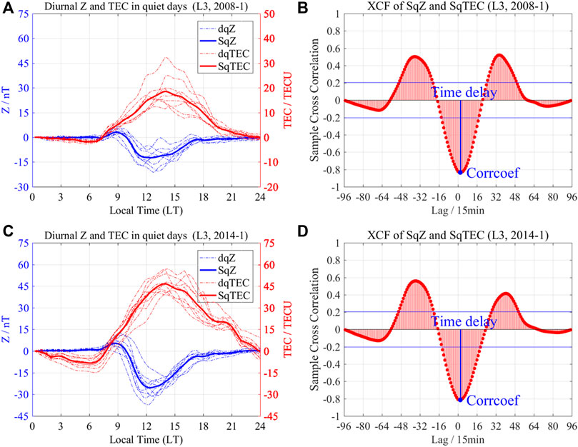
FIGURE 2. Examples of cross-correlation.
In the vast majority of cases, the coefficient at the peak position was negative, so we reasoned a priori that the geomagnetic Z component is correlated negatively with the ionospheric TEC, then we recorded the peak position where the coefficient is negative and minimum. We applied the analytical method to SqZ and SqTEC as well as dqZ and dqTEC. Figure 3 shows the minimum correlation coefficients of dqZ and dqTEC (indicated by red dots) and SqZ and SqTEC (indicated by blue dotted lines) for all stations. This shows that the geomagnetic Z component has a strong negative correlation with TEC, with most of the coefficients being ca. −0.8. Furthermore, Figure 4 shows that the time delays are very large in summer and very small in winter, except for stations M6–M10, and this annual change law is similar in different years at most stations. Therefore, we focus on the seasonal and spatial variations of the time delays.
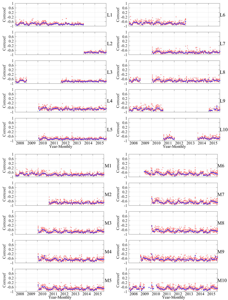
FIGURE 3. Minimum correlation coefficients of dqZ and dqTEC (indicated by red dots) and SqZ and SqTEC (indicated by blue dotted lines).
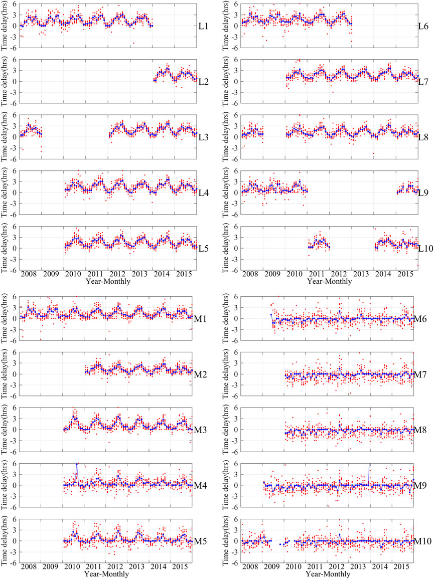
FIGURE 4. Time delays of dqZ and dqTEC (indicated by red dots) and SqZ and SqTEC (indicated by blue dotted lines).
As shown in Figure 4, the differences among the time delays in different years are relatively small, and the monthly variation is much larger than the yearly one. Therefore, we do not consider the yearly difference in the following analysis. Figure 5 shows the averaging time delays of every station in each month. The maximum time delays in Figure 5 appear mainly in August, and the minimum ones appear mainly in January.
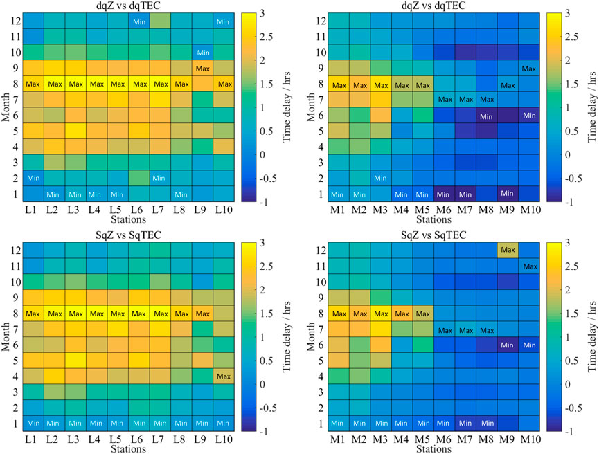
FIGURE 5. Comparison of average time delay in different months.
We use Lloyd’s season division method: May, June, July, and August are summer seasons; January, February, November, and December are winter seasons; and March, April, September, and October are equinox seasons. Figure 6 shows the averaging time delay of every station in each season. This shows that the time delay of every station increases successively in winter, equinox, and summer, and the growth amplitude exceeds 1 h at most stations. The Sq field is strong in local summers and very weak in local winters (Takeda, 2002, 2013a; Vichare et al., 2017), consistent with the seasonal variations of the time delays of SqZ and TEC.
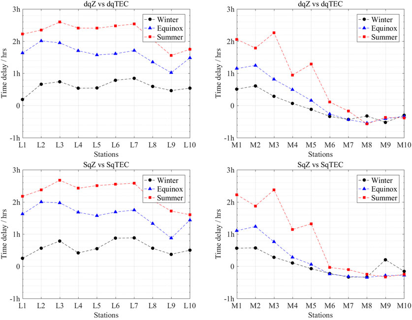
FIGURE 6. Comparison of average time delay in each Lloyd season.
Whether monthly or seasonal variation, the time delay decreases from L1 to M10 and decreases gradually from positive to negative. Therefore, this indicates that the change of Z component is ahead of TEC at low latitudes, but they tend to synchronize with increasing latitude. Also, when the latitude reaches a certain level (ca. 28°N), the change of Z component lags behind TEC (at stations M6–M10). Around 30°N is the latitude at which the center of the Sq current vortex passes with high probability. Therefore, we reason that where the time delay is zero is probably related to the focal location of the Sq current vortex.
Because the difference in time delays between different stations is very small and comparable to the yearly variation, we should account for the effects of different years when analyzing the spatial variation of the time delay. We choose 2011 and 2014 to represent years with different solar activity levels. To analyze the latitudinal dependence of the time delay, we select L1, M1, M4, and M7 because these stations are at similar longitudes but different latitudes and have data in the same year. As shown in Figure 7, the time delay decreases gradually with increasing latitude, and it changes gradually from positive to negative. This is consistent with the aforementioned characteristics. To analyze the longitudinal dependence of the time delay, selecting L10, M2, M1, and M3, and the results are shown in Figure 8. Unlike the latitudinal characteristics, the time delays at different longitudes are similar, indicating that the time delay is influenced mainly by the latitudinal change in spatial distribution. This is because the geomagnetic field and the ionosphere are affected mainly by changes in latitude.
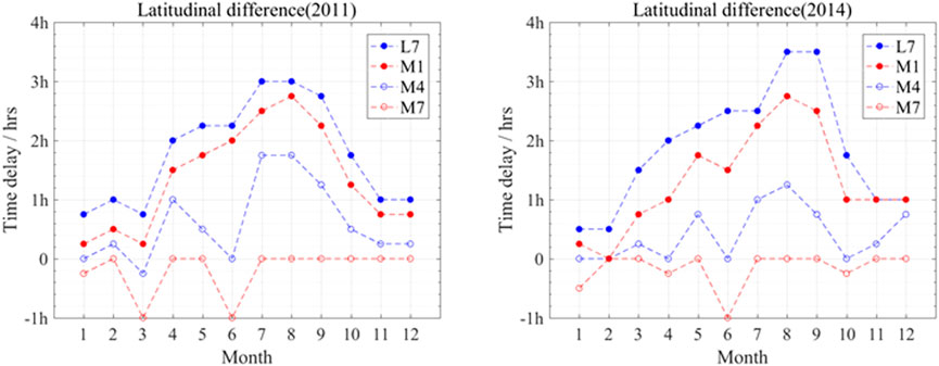
FIGURE 7. Comparison between stations at similar longitudes but different latitudes.
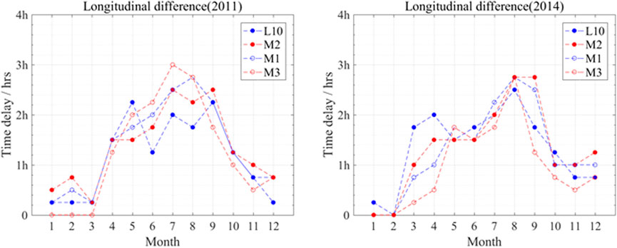
FIGURE 8. Comparison between stations at similar latitudes but different longitudes.
The variation of Sq in the geomagnetic field is mainly caused by the generator current in the ionospheric E layer and its induced current inside the Earth, while the variation of TEC in the ionosphere during the daytime is mainly affected by the photochemical ionization process caused by solar radiation. The variation of the geomagnetic field and the variation of TEC in the ionosphere both originate from solar activity, but they interact with each other through electromagnetic interaction during the variation process. Although there is no causal relationship between ionospheric TEC and the variation of geomagnetic field Sq, the statistical analysis results of SqZ and TEC in this paper show that there is a certain correlation between them in the variation trend.
We analyzed the relationship between the geomagnetic Z component and the ionospheric TEC by investigating their correlation coefficients and time delay, especially the temporal and spatial variations of the time delay. From doing so, we draw the following conclusion.
1) During the geomagnetic quiet days, there is a strong negative correlation between the geomagnetic Z component and the diurnal variation of the ionospheric TEC. Because a negative value of the Z component represents only that its direction is vertically upward, the smaller the value of the Z component, the larger the absolute value, i.e., the strength of the geomagnetic vertical field is larger. Therefore, the strength of the geomagnetic vertical field is related positively to the ionospheric TEC.
2) The time delay between the geomagnetic Z component and the ionospheric TEC has small annual changes but prominent seasonal variations, manifested specifically as being highest in summer, smaller in equinox, and minimum in winter, just like the Sq field strength. The variation of the Z component is ahead of TEC at low latitudes, tends to keep pace with TEC when the latitude increases, and lags behind TEC when the latitude reaches a certain level (ca. 28°N). This suggests that the time delay between SqZ and TEC has some connection to the Sq current vortex position.
The Sq field and ionosphere are both strongly controlled by solar activity. However, in the present study, the relationship between SqZ and ionospheric TEC is similar in both solar-minimum and solar-maximum years. This suggests that their relationship depends not on the Sun but on local position, especially latitude. Also, it emphasizes further the positional sensitivity of the geomagnetic Z component. Therefore, these results indicate that it is reasonable to use the Z component for geomagnetic modeling in geomagnetically assisted navigation, and they provide a theoretical basis for data assimilation or prediction of ionospheric TEC and the Earth’s magnetic field.
The geomagnetic data of this paper comes from the National Geomagnetic Network Center. The ionospheric data comes from the Center for Ionospheric Analysis of the Chinese Academy of Sciences(ftp://ftp.gipp.org.cn/product/ionex/15min/). The magnetic static data is provided by GFZ(ftp://ftp.gfz-potsdam.de/p ub/home/obs/kp-ap/quietdst/).
NC analyzed the time delay between SqZ and TEC, and wrote the paper. WYW downloaded the data, wrote the Section 2 of the paper, and examine the paper. XBY and LXH analyzed cross correlation between SqZ and TEC, and wrote the paper. XM did a great job for the expansion of literature review so as to provide a deeper insight into the related published work.
This work was supported by the National Natural Science Foundation of China (No. 41774156) and the China Postdoctoral Science Foundation (No. 2019M663989).
We were grateful to Prof. Takeda M. and Prof. Xu W. Y. for their insightful suggestions and informative discussions. We acknowledge NGNC, IACA, and GFZ’s open data policy in using geomagnetic data and ionospheric data. We thank the referees for their constructive comments and suggestions.
The authors declare that the research was conducted in the absence of any commercial or financial relationships that could be construed as a potential conflict of interest.
All claims expressed in this article are solely those of the authors and do not necessarily represent those of their affiliated organizations, or those of the publisher, the editors and the reviewers. Any product that may be evaluated in this article, or claim that may be made by its manufacturer, is not guaranteed or endorsed by the publisher.
Biggin, A. J., Steinberger, B., Aubert, J., Suttie, N., Holme, R., Torsvik, T. H., et al. (2013). Possible links between long-term geomagnetic variations and whole-mantle convection processes. Nat. Geosci. 5 (9), 526–533. doi:10.1038/ngeo1521
Briggs, B. H. (1984). The variability of ionospheric dynamo currents. J. Atmos. Terr. Phys. 46 (5), 419–429. doi:10.1016/0021-9169(84)90086-2
Campbell, W. H. (1987). Some effects of quiet geomagnetic field changes upon values used for main field modeling. Phys. Earth Planet. Interiors 48 (3), 193–199. doi:10.1016/0031-9201(87)90144-0
Fujita, S., Murata, Y., Fujii, I., Miyoshi, Y., Shinagawa, H., Jin, H., et al. (2018). Evaluation of the Sq magnetic field variation calculated by GAIA. Space weather. 16 (4), 376–390. doi:10.1002/2017sw001745
He, S. C., Zhang, D. H., Hao, Y. Q., and Xiao, Z. (2020). Statistical study on the occurrence of the ionospheric mid-latitude trough and the variation of trough minimum location over northern hemisphere. Chin. J. Geophys. 63 (1), 31–46. doi:10.6038/cjg2020M0564 (in Chinese).
Jia, J. X., Wang, Y. M., Zhuang, X. Q., Yao, Y., Wang, S. W., Zhao, D., et al. (2017). High spatial resolution shortwave infrared imaging technology based on time delay and digital accumulation method. Infrared Phys. Technol. 81, 305–312. doi:10.1016/j.infrared.2017.01.017
Kuvshinov, A., and Utada, H. (2010). Anomaly of the geomagnetic Sq variation in Japan: Effect from 3-D subterranean structure or the ocean effect. Geophys. J. Int. 183 (3), 1239–1247. doi:10.1111/j.1365-246x.2010.04809.x
Kuvshinov, A. V., Avdeev, D. B., and Pankratov, O. V. (1999). Global induction by Sq and dst sources in the presence of oceans: Bimodal solutions for non-uniform spherical surface shells above radially symmetric Earth models in comparison to observations. Geophys. J. Int. 137 (3), 630–650. doi:10.1046/j.1365-246x.1999.00827.x
Olsen, N. (1996). Magnetospheric contributions to geomagnetic daily variations. Ann. Geophys. 14 (5), 538–544. doi:10.1007/s00585-996-0538-0
Olson, W. P. (1970). Contribution of nonionospheric currents to the quiet daily magnetic variations at the Earth’s surface. J. Geophys. Res. 75 (34), 7244–7249. doi:10.1029/ja075i034p07244
Ou, J. M., Du, A. M., and Christopher, C. F. (2017). Quasi‐biennial oscillations in the geomagnetic field: Their global characteristics and origin. J. Geophys. Res. Space Phys. 122 (5), 5043–5058. doi:10.1002/2016ja023292
Stening, R. J. (2008). The shape of the <I&gt;Sq&lt;/I&gt; current system. Ann. Geophys. 26 (7), 1767–1775. doi:10.5194/angeo-26-1767-2008
Stening, R. J., and Winch, D. E. (2013). The ionospheric Sq current system obtained by spherical harmonic analysis. J. Geophys. Res. Space Phys. 118 (3), 1288–1297. doi:10.1002/jgra.50194
Takeda, M. (2013a). Difference in seasonal and long-term variations in geomagnetic Sq fields between geomagnetic Y and Z components. J. Geophys. Res. Space Phys. 118 (5), 2522–2526. doi:10.1002/jgra.50128
Takeda, M. (2008). Effects of the induction electric field on ionospheric current systems driven by field-aligned currents of magnetospheric origin. J. Geophys. Res. 113, A01306. doi:10.1029/2007ja012662
Takeda, M. (2002). Features of global geomagnetic Sq field from 1980 to 1990. J. Geophys. Res. 107 (A9), 1252. doi:10.1029/2001ja009210
Vasyliunas, V. M. (2012). The physical basis of ionospheric electrodynamics. Ann. Geophys. 30 (2), 357–369. doi:10.5194/angeo-30-357-2012
Vichare, G., Rawat, R., Jadhav, M., and Sinha, A. K. (2017). Seasonal variation of the Sq focus position during 2006-2010. Adv. Space Res. 59 (2), 542–556. doi:10.1016/j.asr.2016.10.009
Xu, W. Y. (1992). Effects of the magnetospheric currents on the Sq-field and a new magnetic index characterizing Sq dynamo current intensity. J. Geomagn. Geoelec. 44 (6), 449–458. doi:10.5636/jgg.44.449
Yamazaki, Y., and Maute, A. (2017). Sq and EEJ—a review on the daily variation of the geomagnetic field caused by ionospheric dynamo currents. Space Sci. Rev. 206 (1–4), 299–405. doi:10.1007/s11214-016-0282-z
Keywords: ionospheric TEC, geomagnetic SqZ, time delay estimation, cross correlation, middle and low latitudes
Citation: Niu C, Wei Y, Xu B, Li X and Mu X (2022) Relationship between ionospheric TEC and geomagnetic SqZ at middle and low latitudes. Front. Astron. Space Sci. 9:1061876. doi: 10.3389/fspas.2022.1061876
Received: 05 October 2022; Accepted: 13 October 2022;
Published: 28 October 2022.
Edited by:
Shufan Zhao, Ministry of Emergency Management, ChinaReviewed by:
Jianxin Jia, Finnish Geospatial Research Institute, FinlandCopyright © 2022 Niu, Wei, Xu, Li and Mu. This is an open-access article distributed under the terms of the Creative Commons Attribution License (CC BY). The use, distribution or reproduction in other forums is permitted, provided the original author(s) and the copyright owner(s) are credited and that the original publication in this journal is cited, in accordance with accepted academic practice. No use, distribution or reproduction is permitted which does not comply with these terms.
*Correspondence: Yiwei Wei, eWl3ZWlfd2VpQDE2My5jb20=
Disclaimer: All claims expressed in this article are solely those of the authors and do not necessarily represent those of their affiliated organizations, or those of the publisher, the editors and the reviewers. Any product that may be evaluated in this article or claim that may be made by its manufacturer is not guaranteed or endorsed by the publisher.
Research integrity at Frontiers
Learn more about the work of our research integrity team to safeguard the quality of each article we publish.