pyGPI5: A python D- and E-region chemistry and ionization model

We present a Python implementation of a D- and E-region chemistry and ionization code called pyGPI5. Particle precipitation that penetrates into the E- and D-region of the ionosphere-thermosphere causes significant enhancements of the electron density. Dissociative recombination of molecular ions with electrons is the primary electron loss mechanism in the E-region, down to approximately 85 km. However, below 85 km, chemical processes become significantly more complicated with positive and negative ions being generated in addition to electrons. The complex D-region ion chemistry has been known for many decades. We present a formulation to quantify the concentrations of four ion species composed of positive and negative, light and heavy ions, and the electrons. The implementation we describe in this investigation solves five ordinary stiff differential equations simultaneously. We present an overview of the code, along with discussions of the reaction rates, and assumptions used in the model. We describe an implementation of the electron transport model to quantify the altitude ionization profile caused by energetic particle precipitation. We show how to instantiate the model, generate the ion and electron profiles as a function of altitude for background conditions, how to generate altitude ionization profiles, and running the code to produce ion and electron profiles caused by energetic particle precipitation. Recent investigations that have used a D-region chemistry model are discussed, along with some applications.

1 Introduction

It has been well-established that the ion chemistry in the D-region of the ionosphere is significantly more complicated than the ion chemistry in the E- or F-regions (Rishbeth and Garriott, 1969; Brekke, 2013). Early rocket observations from ion mass spectrometers resolved positive and negatively charged ions (Narcisi and Bailey, 1965). The D-region electron density has strong impacts on the absorption of high frequency (HF) radio wave propagation (Davies, 1990; Zawdie et al., 2017).

The D-region electron density can be significantly enhanced by energetic particle precipitation. These electron density enhancements can be observed with VLF networks (Cummer et al., 1997; Marshall et al., 2019; Hendry et al., 2020), optical techniques (Marshall et al., 2014; Marshall et al., 2019), at X-ray wavelengths (Marshall et al., 2020), riometers (Marshall and Cully, 2020), and using incoherent scatter radar (Marshall et al., 2014; Miyoshi et al., 2015; Sivadas et al., 2017; Kaeppler et al., 2020; Sanchez et al., 2022). Marshall and Cully (2020) provides an excellent review of observational techniques. However, quantifying observational parameters requires a model that describes the chemistry of the D-region.

There are relatively few models that describe the D-region ion chemistry. To date, the Sodankylä Ion Chemistry (SIC) model is the most comprehensive model of D-region chemistry (Verronen et al., 2005; Turunen et al., 2009; Turunen et al., 2016). SIC is a 1-D vertical transport code that is valid between 20–150 km, with 1 km resolution, and takes into account hundreds of chemical reactions that are driven by solar UV, X-ray, or energetic particle precipitation. SIC solves for the concentrations of at least 65 ions, 36 of which are positive ions, 29 of which are negative ions, and 15 minor neutral species (Turunen et al., 2009, and references therein). There have been recent efforts to incorporate the chemical reactions described in the SIC model into global whole-atmosphere models (Kovács et al., 2016; Verronen et al., 2016).

A second, more simplified, model was originally written by Glukov, Pasko, and Inan (GPI) (Glukhov et al., 1992) which solved four simultaneous differential equations representing the time evolution of the electrons, light positive and negative ions, and heavy positive cluster ions. The GPI model makes the important simplification that ion species and the electrons are modeled as individual fluids; the methodology does not track the evolution of individual ion constituents. The GPI model also does not compute the time evolution of the neutrals. The reaction rates used in the equations are effective reaction rates for the fluid. Lehtinen and Inan (2007) went on to modify the GPI model to include heavy negative cluster ions; therefore, GPI5 solves simultaneously for five ordinary differential equations. Lehtinen and Inan (2007) also made modifications to some of the reaction rates relative to Glukhov et al. (1992).

In this investigation, we present a Python implementation of the GPI5 D-region chemistry and ionization model, which we call pyGPI5. The goal is to produce an open-source, easy-to-use, fast, D-region chemistry and ionization model that is accurate and sufficient for many applications. pyGPI5 provides an implementation of ionization models developed by Fang et al. (2008) and Fang et al. (2010). In Section 2, we present the implementation of the pyGPI5 code, which includes a description of the Python classes. Section 3 presents results which demonstrate various model outputs and basic results. A Jupyter notebook is included in the github repository that shows how the figures for this section were generated. Section 4 presents some recent results that have utilized D-region chemistry codes, not specific to the Python implementation, and demonstrating some applications.

2 Methodology

2.1 Overview

We briefly discuss an overview of the code architecture with an emphasis on the production of electron density. There are two Python classes that compromise the code: the Chemistry class and the Ionization class. The Chemistry class contains the heart of the GPI5 code, in which, five first order stiff ordinary differential equations (ODEs) that describe the time evolution of the electrons, light positive and negative ions, and heavy positive and negative cluster ions are solved simultaneously. The Ionization class produces an altitude ionization profile that is necessary in the equations describing the time evolution of the ions and electrons.

As a forward model, the altitude resolved ionization profile is used as an input. However, in pyGPI5 the inverse problem is solved to produce the background ionization, i.e., given an observed or empirical electron density, the altitude ionization profile is determined. Estimating the differential number flux given the altitude ionization profile is not discussed in this paper, but there are several useful papers that present techniques to address this problem (Semeter and Kamalabadi, 2005; Simon Wedlund et al., 2013; Turunen et al., 2016; Sivadas et al., 2017; Kaeppler et al., 2020).

Before describing the code implementation in more detail, we elaborate on a few important assumptions. First, pyGPI5 is a 1-D model in the vertical component for a given longitude and latitude. The equations described below are solved at each altitude independently and there is no coupling between altitudes. Second, the time evolution of the ion and electron equation is quantified, but each time interval is quantified independently, depending on the ionization profile and the neutral atmospheric parameters. Third, the specification of the neutral atmosphere and corresponding neutral constituents is specified using the NRLMSIS00 model (Picone et al., 2002). pyGPI5 does not solve differential equations describing the time evolution of the neutral species. Fourth, transport effects associated with electric fields and neutral winds are not considered in the continuity equations presented below.

2.2 D-region chemistry class

The heart of the code is contained in the Chemistry class in which five coupled stiff first order differential equations are solved that describe the time evolution of the ions and electrons. The equations from Lehtinen and Inan (2007) that we solve are:

$\frac{d{n}_e}{dt}=q+\gamma n^{-}+{\gamma }_x{n}_x^{-}-\beta n_e-{\alpha }_d{n}_e{n}^{+}-{\alpha }_d^c{n}_e{n}_x^{+}(\mathrm{1a})$

$\frac{d{n}^{-}}{dt}=\beta n_e-\gamma n^{-}-{\alpha }_i{n}^{-}\left(n^{+}+n_x^{+}\right)-\bar{X}{n}^{-}(\mathrm{1b})$

$\frac{d{n}_x^{-}}{dt}=-{\gamma }_x{n}_x^{-}-{\alpha }_i{n}_x^{-}\left(n^{+}+n_x^{+}\right)+\bar{X}{n}^{-}(\mathrm{1c})$

$\frac{d{n}^{+}}{dt}=q-B{n}^{+}-{\alpha }_d{n}_e{n}^{+}-{\alpha }_i{n}^{-}{n}^{+}-{\alpha }_i{n}_x^{-}{n}^{+}(\mathrm{1d})$

$\frac{d{n}_x^{+}}{dt}=-{\alpha }_d^c{n}_e{n}_x^{+}+B{n}^{+}-{\alpha }_i{n}^{-}{n}_x^{+}-{\alpha }_i{n}_x^{-}{n}_x^{+}(1e)$

where Table 1 summarizes the terms found in Eq. 1. These equations are a set of stiff ordinary differential equations that we numerically solve using the Python Scipy ode package. We use the vode integration option with the backward differentiation formulas (bdf) to solve the stiff set of differential equations.

TABLE 1

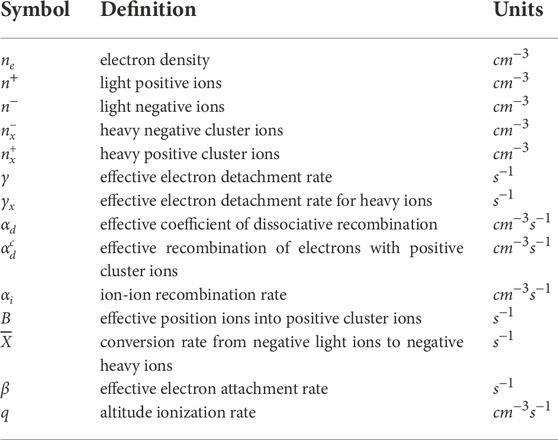
TABLE 1. Variables that are used in Eq. 1.

An observed electron density is composed of both a background electron density and the electron density enhancements caused by energetic particle precipitation or other sources (e.g., solar X-rays, galatic cosmic rays, etc). The background is required as an initial condition upon which the enhanced electron density overlays. We use a bounded bisection method (Press et al., 2007) to derive the ionization profile given an observed electron density or an electron density from a standard model, i.e., the 2016 International Reference Ionosphere (IRI) (Bilitza et al., 2017). At each altitude (z) an iterative process occurs in which, the ionization (q(z)) is varied, the ODEs are solved, and the model electron density is compared to the observations or an empirical specification. For the case of the background electron density, we use the corresponding IRI electron density profile, run the bisection method, and derive the altitude ionization profile. For energetic particle precipitation, the process is the same, but in this case observations are used. We assume that each altitude is independent of other altitudes when running the bisection method.

The reaction rates used in Eq. 1 are found in Glukhov et al. (1992) and Lehtinen and Inan (2007). Many of these reaction rates are dependent on the neutral number density, N_m, as a function of altitude; we use the NRLMSIS00 neutral mass density model for atmospheric specification (Picone et al., 2002). We briefly summarize the reaction rates used, but more details regarding the origin of these coefficients can be found in Glukhov et al. (1992) and Lehtinen and Inan (2007). The effective recombination of electrons with positive cluster ions (n⁺) we use is

${\alpha }_d^c=10^{-5}\left[c{m}^3{s}^{-1}\right](2)$

(Glukhov et al., 1992; Florescu-Mitchell and Mitchell, 2006). The effective ion–ion recombination between positive ions with negative ions is

${\alpha }_i=10^{-7}+N_m\times 10^{-24}\left[c{m}^3{s}^{-1}\right],(3)$

which includes three-body mutual neutralization processes that are important below 40 km altitude (Lehtinen and Inan, 2007, and references therein). The effective electron attachment rate is

$\beta =N_m^{2}5.6\times 10^{-32}\left[c{m}^3{s}^{-1}\right](4)$

which is an approximation for 3-body processes based on the temperature dependent formula found in Glukhov et al. (1992), but evaluated for a specific temperature T = 200K and specified atmospheric concentrations. See Lehtinen and Inan (2007) for more details. The conversion rate from light positive ions, n⁺, to heavy cluster ions $n_x^{+}$ is described by the term B,

$B=N_m^2\times 10^{-31}\left[s^{-1}\right](5)$

The detachment rate of heavy negative ions, γ_x, is defined as γ_x = 0 at night and has a constant rate, γ_x = 0.002, during the day which is primarily due to photodetachment. We define $\bar{X}$ as,

$\bar{X}=0.2\times 10^{-30}{N}_m^2\left[s^{-1}\right](6)$

which corresponds to the conversion rate from light (n⁻) to heavy negative ions.

The effective electron detachment rate, γ, corresponds to the following reaction of O₂,

$O_2^{-}+O_2\to e^{-}+2O_2(7)$

and the default value in the code is specified as

$\gamma =3\times 10^{-17}{N}_m\left[s^{-1}\right](8)$

However, two other options are available. The first option is described by Eq.7 in Lehtinen et al. (1999),

$\gamma =8.61\times 10^{-10}{N}_m{e}^{-6030/T_n}\left[s^{-1}\right](9)$

Where T_n is the neutral temperature. The second option is a slightly modified equation derived by (Kozlov et al., 1988)

$\gamma =2.7\times 10^{-10}{N}_m{e}^{-5590/T_n}\sqrt{\left(\frac{T_n}{300}\right)}\left[s^{-1}\right](10)$

The neutral temperature, T_n, needed in both calculations is provided by the NRLMSISE00 model.

pyGPI5 has been modified to include chemistry in the E-region of the ionosphere. In the E-region, the primary loss process is dissociative recombination (α_d) of the dominant molecular ions NO⁺ and ${\mathrm{O}}_2^{+}$ (Schunk and Nagy, 2004). The GPI5 code originally used a constant recombination rate for α_d. However for pyGPI5, we use the following recombination rates for NO⁺ and ${\mathrm{O}}_2^{+}$ (Schunk and Nagy, 2004), for Te < 1200 K:

$\begin{array}{cc}\hfill {\alpha }_{O_2^{+}}& =1.95\times 10^{-7}{\left(300/T_e\right)}^{0.70}\left[c{m}^3{s}^{-1}\right]\hfill \\ \hfill {\alpha }_{N{O}^{+}}& =3.50\times 10^{-7}{\left(300/T_e\right)}^{0.69}\left[c{m}^3{s}^{-1}\right]\hfill \end{array}(11)$

and for T_e > 1200 K:

$\begin{array}{cc}\hfill {\alpha }_{O_2^{+}}& =1.95\times 10^{-7}{\left(300/T_e\right)}^{0.56}\left[c{m}^3{s}^{-1}\right]\hfill \\ \hfill {\alpha }_{N{O}^{+}}& =3.02\times 10^{-7}{\left(300/T_e\right)}^{0.56}\left[c{m}^3{s}^{-1}\right]\hfill \end{array}(12)$

where T_e is the electron temperature from IRI2016. These two recombination rates are weighted using the relative concentrations of NO⁺ and ${\mathrm{O}}_2^{+}$:

$\alpha \left(z\right)=\sum _{i}I{c}_i\left(z\right){\alpha }_i\left(z\right)(13)$

where Ic_i corresponds to the ion concentration that can be taken from IRI2016 which internally derives these values from the FLIP ion chemistry model (Richards et al., 2010).

There is one free parameter that is required to solve Eq. 1 which is the equation integration time, or the end time for the integration of the ODEs. The chemistry interactions are very rapid in the D-region, with steady-state conditions being achieved of the order of seconds or less; while in the E-region, 1–10 s of seconds is considered a pretty typical steady-state interval (Semeter and Kamalabadi, 2005). For example, Marshall et al. (2014) shows a 5 MeV 0.1A beam that has a peak electron density enhancement at 44 km, but the recovery time to ambient levels occurs of the order of 10–100 ms. These fundamental recovery time are the basis for the choice of the integration time, although the integration scheme should have time steps that are significantly shorter than the characteristic recovery time. However, in some cases, an appropriate integration time may depend on the application for which the code is being used or on another constraint, such as, the time interval associated with the observations. For the case of ISR, the collection time of the radar, i.e., the integration interval, is typically significantly longer and of the order of 10–300 s for most experiments. Therefore, it makes sense to use the longer integration interval for the equations when comparing to ISR observations. A recent experiment by Bernhardt et al. (2022) examined the decay of the electron density from stimulated VLF emissions using rocket engines, which were of the order of 15–240 s.

2.3 Ionization class

The second class in pyGPI5 is the Ionization class. Fang et al. (2008) and Fang et al. (2010) derived an easy-to-calculate electron transport model. Fang et al. (2008) derived the parameterization assuming that the precipitating electron energy flux was characterized by a Maxwellian distribution. Fang et al. (2010) expanded upon Fang et al. (2008) by relaxing the Maxwellian assumption and using monoenergetic beams thus enabling the use of other data sets (i.e., satellite data) with discrete energies. Effectively, Fang et al. (2008) and Fang et al. (2010) solved the following equations,

$q\left(z\right)=\frac{Q_0}{2\mathrm{\Delta }ϵ}\frac{f\left(y,E_0\right)}{H\left(z\right)}(\mathrm{14a})$

$f\left(y,E_0\right)=C_1{y}^{C_2}\exp \left(-C_3{y}^{C_4}\right)+C_5{y}^{C_6}\exp \left(-C_7{y}^{C_8}\right)(\mathrm{14b})$

$y=\frac{1}{E_0}{\left(\frac{\rho \left(z\right)H\left(z\right)}{{\alpha }_0}\right)}^{{\beta }_0}(\mathrm{14c})$

$C_i=\exp \left(\sum _j{P}_{ij}\ln {\left(E_0\right)}^j\right)(\mathrm{14d})$

where Δϵ is the ion-pair production energy (i.e., 35 eV), Q₀ is the energy flux, H(z) = k_BT_n(z)/m(z)g(z) is the atmospheric scale height, ρ(z) is the atmospheric mass density given by NRLMSIS00, and α₀ is a constant. P_ij and β₀ are fit parameters that depend on whether the incident differential number flux is a Maxwellian distribution (Fang et al., 2008) or monoenergetic (Fang et al., 2010), and are not repeated here.

A key model which will be implemented in future versions of pyGPI5 is the Boulder Electron Radiation to Ionization (BERI) model (Xu et al., 2020). BERI was developed as an easy-to-calculate ionization model that included pitch angle effects and is valid for energies of 3 keV–33 MeV. This model was specifically designed to address whether pitch angle effects had important consequences in D-region and mesosphere chemistry. In addition, other transport models can be implemented in pyGPI5. For a summary of other transport models, we refer the read to the monograph by Kaeppler et al. (2020).

2.4 Comparisons with Sodankylä ion chemistry

The GPI5 implementation has been compared with results from the SIC model in a few limited cases. Figure 3 (not shown here) in Marshall et al. (2019) presents a comparison of the two models for the case of a 1 MeV electron beam delivering 1 kJ over 100 pulses every 5 ms. The comparison shows that the altitude of the peak electron density of the GPI5 model was 60 km, while the peak altitude for the SIC model was 61 km. Additionally, the SIC model predicted a peak electron density that was 50% larger than the GPI5 model. In spite of the differences the overall agreement between both models is favorable. An area of future effort could be more systematic comparisons between GPI5 and the SIC model.

3 Results

We present examples of different implementations within pyGPI5. The figures below can be generated in the RunExamples.ipynb Jupyter notebook. The results presented were collected with the Poker Flat Incoherent Scatter Radar (PFISR) (65.13°N and 147.47°W) for 08 May 2018 at 0500 UTC. This interval and location were chosen to be similar to an event of energetic particle precipitation presented in Sanchez et al. (2022). The geomagnetic conditions associated with this time interval were Dst = -30 nT and Kp = 2 (Sanchez et al., 2022). We present results from 60 to 150 km altitudes at 1 km altitude resolution.

Figure 1 presents reaction rates described in Table 1 that are necessary to solve Eq. 1. The left column shows the recombination rates and the right column presents the other coefficients, both columns are separated by units. For the effective recombination rate, α_d, at approximately 75 km, the concentrations of NO⁺ and $O_2^{+}$ both go to zero, thus resulting in the effective recombination rate going to zero at this altitude. Above 100 km, we see that the recombination rate has a nearly exponential decrease with respect to altitude, which is similar to previous investigations (Vickrey et al., 1982; Gledhill, 1986). The altitude profile of β, B, and $\bar{X}$ are similar to the NRLMSIS00 neutral mass density, as expected.

FIGURE 1

FIGURE 1. Altitude profiles of the coefficients used in Eq. 1. The left column shows the recombination rates with units of cm³s⁻¹ and the right column shows other reaction rates which have units of s⁻¹. The profiles are shown from 60 to 150 km altitudes at the location of the Poker Flat Incoherent Scatter Radar (PFISR) on 08 May 2018 at 0500 UTC.

Figure 2 shows the altitude ionization profiles for a monoenergetic flux and a Maxwellian energy distribution. The altitude ionization profiles caused by the monoenergetic energy flux described in Fang et al. (2010), while for the Maxwellian energy flux we used the Fang et al. (2008) implementation. In both cases, the same input energy flux of 1 mW/m² was used, but different monoenergetic beam energies or characteristic energy for the Maxwellian flux were used.

FIGURE 2

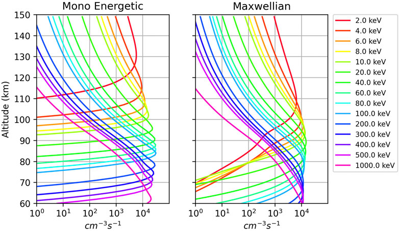
FIGURE 2. The altitude ionization rates for monoenergetic and Maxwellian flux distributions in the left and right columns, respectively. The monoenergetic beam energy and characteristic energy of the Maxwellian distribution are shown in the caption. Both of these cases use a 1 mW/m² energy flux.

The peak altitude of the electron density for the Maxwellian flux distribution occurs at a lower altitude relative to the monoenergetic beam with the same energy. For example, the altitude of the peak electron density for the 2 keV monoenergetic beam is approximately 125 km, while the peak altitude for the 2 keV Maxwellian distribution is approximately 107 km. The Maxwellian distribution has a characteristic energy, E₀, which corresponds to the energy at which the peak flux occurs. However, the average energy ⟨E⟩ is used instead because it is a figure of merit that is independent of the spectral shape of the differential energy flux. For the a Maxwellian, ⟨E⟩ = 2E₀ (Robinson et al., 1987), and the energy in the legend of Figure 2 corresponds to the characteristic energy. If we compare the peak altitude of 2 keV Maxwellian flux with the 4 keV monoenergetic beam, the altitudes are much closer to each other, which is consistent with the difference between the average energy and the characteristic energy.

Figure 3 shows altitude profiles for the light and heavy positive and negative ions, and the electrons, respectively. The left column shows the altitude profiles for background conditions, which correspond to an IRI run on 08 May 2018 at 0500 UT. As stated in Section 2.2, Eq. 1 is solved in steady state to produce the light and heavy ion and electron profiles. The right column shows the response of the electron density caused by a 300 keV monoenergetic beam with a 1 mW/m² energy flux. The light positive ions, n⁺, are the dominant ion species down to 85 km, and approximately match in magnitude with the electron density. The response we observe is what would be expected for chemistry with molecular ions in the E-region of the ionosphere. Below 85 km, for the background case the positive light ions, positive heavy ions, and negative heavy ions have similar magnitudes. These species work together to cause the electron density to be lower than simply the positive light ions contribution alone.

FIGURE 3

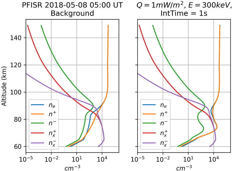
FIGURE 3. The altitude profiles of the positive and negative heavy and light ions, and the electrons. The left column shows the altitude profiles for the background, corresponding to IRI, at PFISR on 08 May 2018 at 0500 UT. The right panel shows the same time interval, but now including a monoenergetic beam with energy 300 keV and an energy flux of 1 mW/m². The equations are integrated for 1 s.

During the case of enhanced ionization from the energetic particle precipitation the electron density has a peak at ∼ 75 km altitude. The peak altitude of the electron density is consistent with the altitude of the peak ionization shown in Figure 2. The electron density above 100 km altitude is unaffected by the energetic precipitation since the peak altitude of the ionization is below 80 km. The light positive ions approximately balance the electrons at all altitudes. This is partially a consequence of Eq. 1a and Eq. 1d), since both of these equations contain the altitude ionization profile represented by q. Although we note that a secondary peak in the negative light ions has developed at ∼ 75 km altitude during the energetic precipitation, eventhough it is 1-2 orders of magnitude smaller than the positive light ions. The heavy positive and negative ions have the largest magnitude below 85 km, although there is no difference between the background versus interval with particle precipitation. However, it is important to note that the cluster ions have effectively equal and opposite total charge, so these species do not impact the electron density or the light ions. The lack of difference is due to the coefficients being fixed by the empirical specification of the neutral mass density, which does not evolve in time.

Figure 4 shows how the electron density varies as a function of integration time (end time) for three monoenergetic beam energies. Each column shows a monoenergetic beam with an energy flux of 1 mW/m² but different energies corresponding to 300 keV, 50 keV, and 10 keV in the left, middle, and right columns, respectively. We chose a set of integration times to show the evolution and 300s (5 min) being a typical time interval associated with ISR experiments. For the 300 keV energy, the peak altitude moves up from 75 km to 80 km between 10 s and 60 s. We also find that 60 s of integration has reached a steady-state configuration, since there is little difference between the electron density profile at 60 s or 300 s. We find in all cases that going from 1 s to 5 s of integration seems to change the electron density profile significantly. For the 50 keV beam, steady-state has nearly been achieved between 5 and 10 s, and similarly for the 10 keV beam; one conclusion we can draw is that 10 s is nearly steady-state for energies above 100 keV. The peak for the 50 keV and 10 keV beams occurs at just below 90 km and near 100 km altitude, respectively.

FIGURE 4

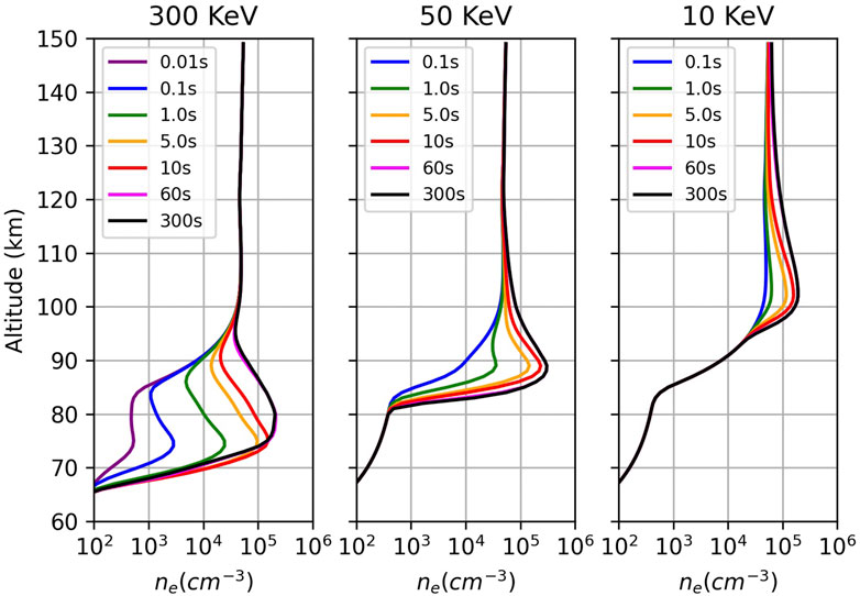
FIGURE 4. The electron density vs. altitude is plotted to show the relaxation time for a monoenergetic flux at 300 keV, 50 keV, and 10 keV shown as the left, middle, and right columns, respectively. All examples have an energy flux of 1 mW/m². We find that the 50 keV and 10 keV beams come into near steady state after 10 s, while the 300 keV beam takes 60 s.

4 Discussion and applications

We present recent examples that have used the GPI5 formulation. Marshall et al. (2014) and Marshall et al. (2019) quantify ground-based observables (i.e., electron density, photons, etc.) caused by a beam of energetic electrons driven by a linear accelerator. Both papers modeled optical emission, X-rays, and electron density enhancements that could be measured with ISR. Marshall and Cully (2020) also modeled subionospheric VLF signatures that would be modified by energetic particle preciptiation. The GPI5 framework provides ion and electron densities which can be used to calculate light emission, VLF propagation, or used directly, as in the case of ISR.

Sanchez et al. (2022) presents an observational study of energetic particle precipitation observed with the Poker Flat Incoherent Scatter Radar for an event on 8 May 2018. During this event there were near conjunctions ($<$ 500 km) between the Van Allen Probes satellites A and B and PFISR, thus enabling the electromagnetic wave fields to be observed nearly simultaneously relative to ground-based observations of the precipitation. The satellite electromagnetic wave data were predominantly chorus waves, which were used in quasi-linear diffusion codes to produce enhanced pitch angle scatter diffusion rates and the loss cone population. The BERI code was then used to produce observable signatures which were compared with the PFISR observations of electron density. Ma et al. (2022) presents similar results to Sanchez et al. (2022), but instead using near conjunctions between the Arase satellite and PFISR. In this case, Ma et al. (2022) found cases where plasmaspheric hiss was generating energetic precipitation that was observed with PFISR.

Bernhardt et al. (2022) demonstrated how rocket motors can impact the local plasma environment that can energize ions. The energized ions cause significant enhancement in VLF emission, which enhance wave particle interactions and thus generate energetic particle precipitation. Bernhardt et al. (2022) used the SIC model to model the D-region ionospheric response as a result of the energetic precipitation, which is detectable using ISR. They also modeled the impacts to subionospheric VLF propagation were also shown for a notional NLK transmitter to a receiver located in Dover DE.

Bernhardt et al. (2022) also calculated the impact that D-region electron density enhancements have on the absorption of high frequency radio wave propagation at 30 MHz, consistent with what one might expect to observe with a riometer. Recently, Zawdie et al. (2017) presented a review of methods for calculating the absorption rate of HF radio waves. Eq. 3 from Zawdie et al. (2017) presents the complex part of the wavevector, k = k_r + iκ,

$\kappa =\frac{e^2}{2{ϵ}_{0}mc}\frac{1}{\mu }\frac{n_e{\nu }_e}{{\nu }_e^2+{\left(2\pi f\pm {\mathrm{\Omega }}_e\cos \theta \right)}^2}(15)$

where ν_e is the electron collision frequency, Ω_e is the electron cyclotron frequency, θ is the angle between k and the magnetic field B₀, and f is the frequency of the transmitter. The plus/minus sign corresponds to ordinary (O-mode) and extraordinary (X-mode) propagation, respectively. Deviate absorption corresponds to the case when n_eν_en is large, and clearly this case is achieved during energetic particle precipitation (Davies, 1990). The pyGPI5 model provides a suitable means to model the D-region electron density enhancements.

5 Summary and conclusion

We present an open source python code base, pyGPI5, designed to quantify the vertical profile of light and heavy positive and negative ions and electrons in the D- and E-region of the ionosphere. An important distinction of this model is that the ions and electrons are treated as single fluids and the chemical reaction rates are represented by effective rates. The formulation in the pyGPI5 model is in contrast to the Sodankylä Ion Chemistry model, which tracks the time evolution of specific ions. pyGPI5 solves five simultaneous coupled stiff ordinary differential equations, corresponding to heavy and light positive and negative ions, plus electrons. However, pyGPI5 does not solve differential equations describing the time evolution of the neutral species.

We present an overview of the code architecture, including the two dominant python classes that comprise the code. The Chemistry class solves the time evolution of the light and heavy ions and electrons. The reaction rates used in the code are presented. The Ionization class generates an altitude ionization profile which is a necessary input for the five differential equations and can change depending on the driving precipitation. For the ionization profiles, we implemented the Fang et al. (2008) and Fang et al. (2010) models for Maxwellian and monoenergetic beams, respectively. A future step will be to implement the Boulder Electron Radiation to Ionization model that describes the electron precipitation. Other ionospheric models, neutral atmospheric models, and transport codes could be implemented within the framework of pyGPI5.

We present results showing different model outputs. The figures presented in the results section are contained within a Jupyter notebook that is on the github page. We show how to instantiate the model, generate the altitude ion and electron profiles for background conditions, how to generate altitude ionization profiles, and how to generate the ion and electron profiles corresponding to energetic particle precipitation. We also show how the peak electron density changes for characteristic relaxation times. We present recent results that have used D-region chemistry models and including a few applications that require a D-region chemistry model, such as, absorption of high frequency radio waves.

In conclusion, we present the pyGPI5 model and the source code as a straight-forward model to generate D- and E-region ion and electron profiles as a function of altitude. We have additionally presented assumptions and caveats that the user should be aware of when running this code for a given application. We also emphasize once again that this model does have some significant simplifications and if the topics of interest require an understanding of the evolution of a specific ion species, other models are better suited to address those needs, such as the Sodankylä Ion Chemistry model.

Data availability statement

The datasets presented in this study can be found in online repositories. The names of the repository/repositories and accession number(s) can be found below: [https://github.com/srkaeppler/pyGPI5].

Author contributions

SK drafted the text and the figures presented in this investigation. RM and DJ provided the original GPI code which was translated to python and suggested code edits for the current version. ES was the PI of the NSF grant that partially funded this work and has provided useful input to the manuscript. AJ and RT have provided important code edits and useful input to the manuscript.

Funding

ES, RM, and SK were funded by NSF Collaborative Research Grant AGS–1732365. SK was additionally funded by Air Force Office of Scientific Research Grant FA9550-19-1-0130.

Conflict of interest

The authors declare that the research was conducted in the absence of any commercial or financial relationships that could be construed as a potential conflict of interest.

Publisher’s note

All claims expressed in this article are solely those of the authors and do not necessarily represent those of their affiliated organizations, or those of the publisher, the editors and the reviewers. Any product that may be evaluated in this article, or claim that may be made by its manufacturer, is not guaranteed or endorsed by the publisher.

References

Bernhardt, P. A., Hua, M., Bortnik, J., Ma, Q., Verronen, P. T., McCarthy, M. P., et al. (2022). Active precipitation of radiation belt electrons using rocket exhaust driven amplification (reda) of man-made whistlers. J. Geophys. Res. Space Phys. 127, e2022JA030358. doi:10.1029/2022ja030358

PubMed Abstract | CrossRef Full Text | Google Scholar

Bilitza, D., Altadill, D., Truhlik, V., Shubin, V., Galkin, I., Reinisch, B., et al. (2017). International reference ionosphere 2016: From ionospheric climate to real-time weather predictions. Space weather. 15, 418–429. doi:10.1002/2016SW001593

CrossRef Full Text | Google Scholar

Brekke, A. (2013). The ionosphere. Berlin, Heidelberg: Springer Berlin Heidelberg.

Google Scholar

Cummer, S. A., Bell, T. F., Inan, U. S., and Chenette, D. L. (1997). Vlf remote sensing of high-energy auroral particle precipitation. J. Geophys. Res. 102, 7477–7484. doi:10.1029/96JA03721

CrossRef Full Text | Google Scholar

Davies, K. (1990). Ionospheric radio. Electromagnetic waves. London, United Kingdom: The Institution of Engineering and Technology.

Google Scholar

Fang, X., Randall, C. E., Lummerzheim, D., Solomon, S. C., Mills, M. J., Marsh, D. R., et al. (2008). Electron impact ionization: A new parameterization for 100 ev to 1 mev electrons. J. Geophys. Res. 113, n/a. doi:10.1029/2008JA013384.A09311

CrossRef Full Text | Google Scholar

Fang, X., Randall, C. E., Lummerzheim, D., Wang, W., Lu, G., Solomon, S. C., et al. (2010). Parameterization of monoenergetic electron impact ionization. Geophys. Res. Lett. 37, n/a. doi:10.1029/2010gl045406

CrossRef Full Text | Google Scholar

Florescu-Mitchell, A., and Mitchell, J. (2006). Dissociative recombination. Phys. Rep. 430, 277–374. doi:10.1016/j.physrep.2006.04.002

CrossRef Full Text | Google Scholar

Gledhill, J. A. (1986). The effective recombination coefficient of electrons in the ionosphere between 50 and 150 km. Radio Sci. 21, 399–408. doi:10.1029/RS021i003p00399

CrossRef Full Text | Google Scholar

Glukhov, V. S., Pasko, V. P., and Inan, U. S. (1992). Relaxation of transient lower ionospheric disturbances caused by lightning-whistler-induced electron precipitation bursts. J. Geophys. Res. 97, 16971–16979. doi:10.1029/92JA01596

CrossRef Full Text | Google Scholar

Hendry, A. T., Clilverd, M. A., Rodger, C. J., and Engebretson, M. J. (2020). “Chapter 8 - ground-based very-low-frequency radio wave observations of energetic particle precipitation,” in The dynamic loss of earth’s radiation belts. Editors A. N. Jaynes, and M. E. Usanova (Elsevier), 257–277. doi:10.1016/B978-0-12-813371-2.00008-1

CrossRef Full Text | Google Scholar

Kaeppler, S. R., Sanchez, E., Varney, R. H., Irvin, R. J., Marshall, R. A., Bortnik, J., et al. (2020). “Chapter 6 - incoherent scatter radar observations of 10–100kev precipitation: Review and outlook,” in The dynamic loss of earth’s radiation belts. Editors A. N. Jaynes, and M. E. Usanova (Elsevier). doi:10.1016/B978-0-12-813371-2.00006-8

CrossRef Full Text | Google Scholar

Kovács, T., Plane, J. M. C., Feng, W., Nagy, T., Chipperfield, M. P., Verronen, P. T., et al. (2016). D-region ion–neutral coupled chemistry (Sodankylä Ion Chemistry, SIC) within the whole atmosphere community climate model (WACCM 4) – WACCM-SIC and WACCM-rSIC. Geosci. Model Dev. 9, 3123–3136. doi:10.5194/gmd-9-3123-2016

CrossRef Full Text | Google Scholar

Kozlov, S. I., Vlaskov, V. A., and Smirnova, N. V. (1988). Speicalized aeronomic model for investigating artifical midification of the middle atmosphere and lower ionosphere. 1. requires for the model and basic concepts of its formation. Cosm. Res. Engl. Transl. 26, 635–642.

Google Scholar

Lehtinen, N. G., and Inan, U. S. (2007). Possible persistent ionization caused by giant blue jets. Geophys. Res. Lett. 34, n/a. doi:10.1029/2006gl029051

CrossRef Full Text | Google Scholar

Lehtinen, N. G., Bell, T. F., and Inan, U. S. (1999). Monte Carlo simulation of runaway MeV electron breakdown with application to red sprites and terrestrial gamma ray flashes. J. Geophys. Res. 104, 24699–24712. doi:10.1029/1999JA900335

CrossRef Full Text | Google Scholar

Ma, Q., Xu, W., Sanchez, E. R., Marshall, R. A., Bortnik, J., Reyes, P. M., et al. (2022). A test of energetic particle precipitation models using simultaneous incoherent scatter radar and van allen probes observations. J. Geophys. Res. Space Phys. 127, e2021JA030179. e2022JA030545. doi:10.1029/2021JA030179

PubMed Abstract | CrossRef Full Text | Google Scholar

Marshall, R. A., and Cully, C. M. (2020). “Chapter 7 - atmospheric effects and signatures of high-energy electron precipitation,” in The dynamic loss of earth’s radiation belts. Editors A. N. Jaynes, and M. E. Usanova (Elsevier). doi:10.1016/B978-0-12-813371-2.00007-X

CrossRef Full Text | Google Scholar

Marshall, R. A., Nicolls, M., Sanchez, E., Lehtinen, N. G., and Neilson, J. (2014). Diagnostics of an artificial relativistic electron beam interacting with the atmosphere. J. Geophys. Res. Space Phys. 119, 8560–8577. doi:10.1002/2014JA020427

CrossRef Full Text | Google Scholar

Marshall, R. A., Xu, W., Kero, A., Kabirzadeh, R., and Sanchez, E. (2019). Atmospheric effects of a relativistic electron beam injected from above: Chemistry, electrodynamics, and radio scattering. Front. Astron. Space Sci. 6. doi:10.3389/fspas.2019.00006

CrossRef Full Text | Google Scholar

Marshall, R. A., Xu, W., Woods, T., Cully, C., Jaynes, A., Randall, C., et al. (2020). The aepex mission: Imaging energetic particle precipitation in the atmosphere through its bremsstrahlung x-ray signatures. Adv. Space Res.Advances Small Satell. Space Sci. 66, 66–82. doi:10.1016/j.asr.2020.03.003

CrossRef Full Text | Google Scholar

Miyoshi, Y., Oyama, S., Saito, S., Kurita, S., Fujiwara, H., Kataoka, R., et al. (2015). Energetic electron precipitation associated with pulsating aurora: Eiscat and van allen probe observations. J. Geophys. Res. Space Phys. 120, 2754–2766. doi:10.1002/2014ja020690

CrossRef Full Text | Google Scholar

Narcisi, R. S., and Bailey, A. D. (1965). Mass spectrometric measurements of positive ions at altitudes from 64 to 112 kilometers. J. Geophys. Res. 70, 3687–3700. doi:10.1029/JZ070i015p03687

CrossRef Full Text | Google Scholar

Picone, J. M., Hedin, A. E., Drob, D. P., and Aikin, A. C. (2002). NRLMSISE-00 empirical model of the atmosphere: Statistical comparisons and scientific issues. J. Geophys. Res. 107, SIA 15-21–SIA 15-16. doi:10.1029/2002JA009430

CrossRef Full Text | Google Scholar

Press, W., Teukolsky, S., Vetterling, W., and Flannery, B. (2007). Numerical recipes 3rd edition: The art of scientific computing. Numerical recipes: The art of scientific computing. New York, NY: Cambridge University Press.

Google Scholar

Richards, P. G., Bilitza, D., and Voglozin, D. (2010). Ion density calculator (idc): A new efficient model of ionospheric ion densities. Radio Sci. 45, n/a. doi:10.1029/2009rs004332

CrossRef Full Text | Google Scholar

Rishbeth, H., and Garriott, O. K. (1969). Introduction to ionospheric physics. Academic Press: New York, NY.

Google Scholar

Robinson, R. M., Vondrak, R. R., Miller, K., Dabbs, T., and Hardy, D. (1987). On calculating ionospheric conductances from the flux and energy of precipitating electrons. J. Geophys. Res. 92, 2565–2569. doi:10.1029/JA092iA03p02565

CrossRef Full Text | Google Scholar

Sanchez, E. R., Ma, Q., Xu, W., Marshall, R. A., Bortnik, J., Reyes, P., et al. (2022). A test of energetic particle precipitation models using simultaneous incoherent scatter radar and van allen probes observations. J. Geophys. Res. Space Phys. 127, e2021JA030179. doi:10.1029/2021ja030179

PubMed Abstract | CrossRef Full Text | Google Scholar

Schunk, R. W., and Nagy, A. F. (2004). Ionospheres. New York, NY: Cambridge University Press.

Google Scholar

Semeter, J., and Kamalabadi, F. (2005). Determination of primary electron spectra from incoherent scatter radar measurements of the auroralEregion. Radio Sci. 40, RS2006. doi:10.1029/2004RS003042

CrossRef Full Text | Google Scholar

Simon Wedlund, C., Lamy, H., Gustavsson, B., Sergienko, T., and BräNdströM, U. (2013). Estimating energy spectra of electron precipitation above auroral arcs from ground-based observations with radar and optics. J. Geophys. Res. Space Phys. 118, 3672–3691. doi:10.1002/jgra.50347

CrossRef Full Text | Google Scholar

Sivadas, N., Semeter, J., Nishimura, Y., and Kero, A. (2017). Simultaneous measurements of substorm-related electron energization in the ionosphere and the plasma sheet. JGR. Space Phys. 122, 547. doi:10.1002/2017ja023995

CrossRef Full Text | Google Scholar

Turunen, E., Verronen, P. T., Seppälä, A., Rodger, C. J., Clilverd, M. A., Tamminen, J., et al. (2009). Impact of different energies of precipitating particles on nox generation in the middle and upper atmosphere during geomagnetic storms. J. Atmos. Sol. Terr. Phys.High Speed Sol. Wind Streams Geosp. Interact. 71, 1176–1189. doi:10.1016/j.jastp.2008.07.005

CrossRef Full Text | Google Scholar

Turunen, E., Kero, A., Verronen, P. T., Miyoshi, Y., Oyama, S.-I., and Saito, S. (2016). Mesospheric ozone destruction by high-energy electron precipitation associated with pulsating aurora. JGR. Atmos. 121, 11. doi:10.1002/2016jd025015

CrossRef Full Text | Google Scholar

Verronen, P. T., SeppäLä, A., Clilverd, M. A., Rodger, C. J., KyröLä, E., Enell, C.-F., et al. (2005). Diurnal variation of ozone depletion during the October-November 2003 solar proton events. J. Geophys. Res. 110, A09S32. doi:10.1029/2004JA010932

CrossRef Full Text | Google Scholar

Verronen, P. T., Andersson, M. E., Marsh, D. R., Kovács, T., and Plane, J. M. C. (2016). Waccm-d—Whole atmosphere community climate model with d-region ion chemistry. J. Adv. Model. Earth Syst. 8, 954–975. doi:10.1002/2015MS000592

CrossRef Full Text | Google Scholar

Vickrey, J. F., Vondrak, R. R., and Matthews, S. J. (1982). Energy deposition by precipitating particles and Joule dissipation in the auroral ionosphere. J. Geophys. Res. 87, 5184–5196. doi:10.1029/JA087iA07p05184

CrossRef Full Text | Google Scholar

Xu, W., Marshall, R. A., Tyssøy, H. N., and Fang, X. (2020). A generalized method for calculating atmospheric ionization by energetic electron precipitation. J. Geophys. Res. Space Phys. 125, e2020JA028482. doi:10.1029/2020ja028482

CrossRef Full Text | Google Scholar

Zawdie, K. A., Drob, D. P., Siskind, D. E., and Coker, C. (2017). Calculating the absorption of hf radio waves in the ionosphere. Radio Sci. 52, 767–783. doi:10.1002/2017RS006256

CrossRef Full Text | Google Scholar