The Lompe code: A Python toolbox for ionospheric data analysis

A recent paper by Laundal et al. (2022c) presented a new technique to combine all available measurements of polar ionospheric electrodynamics; magnetic field measurements from ground and space, ionospheric convection data from radars and satellites, and conductance measurements; to a full 2D map within analysis regions of arbitrary resolution and extent. The technique, called Local Mapping of Polar Ionospheric Electrodynamics (Lompe), is implemented in Python (Laundal et al., 2022a). The Lompe technique combines spherical elementary current system analysis, finite element analysis on a cubed-sphere projection, the use of empirical models like the International Geomagnetic Reference Field, and visualization tools. In this paper, we go through these different components of the Lompe code and show how they are useful on their own, for example in the analysis of ground magnetometer data or data from the upcoming Electrojet Zeeman Imaging Explorer mission. We also demonstrate how to use the Lompe code to produce a coherent picture of ionospheric electrodynamics.

1 Introduction

The Local mapping of polar ionospheric electrodynamics (Lompe) technique (Laundal et al., 2022c) combines all relevant data points in a region of interest to produce a 2D map of ionospheric electrodynamics. Given a map of the ionospheric conductance, Lompe can be fed magnetic field measurements from ground and/or space, and any type of electric field or F-region ionospheric convection measurement and output a continuous map of ionospheric electrodynamics: The electric field, plasma flow, ionospheric horizontal and field-aligned current (FAC), and associated magnetic field perturbations on ground and in space. It is conceptually similar to the Assimilative Mapping of Ionospheric Electrodynamics (AMIE) technique (Richmond and Kamide, 1988; AMGeO Collaboration, 2019), but it uses a different set of basis functions: While AMIE uses spherical cap harmonics that span the entire region poleward of some latitude (usually set to 50°), Lompe represents ionospheric electrodynamics with spherical elementary current systems (SECS; Amm, 1997), which in principle allows more flexibility in choosing the spatial resolution and extent of the analysis region. The Lompe technique is open-source (Laundal et al., 2022a). It is implemented entirely in Python and optimized by using NumPy array operations instead of Python loops where possible. This makes the code portable, user-friendly, and easy to interface with extensive scientific Python modules like NumPy, SciPy, Matplotlib, and Pandas, without a big loss in performance compared to compiled languages.

The Lompe Python package includes several submodules which are required to carry out the Lompe inversion, but are also useful on their own in many aspects of ionospheric data analysis. In this paper, we go through the main components of the Lompe code and present examples of how they can be used. Except for Figure 6, all figures in this paper are outputs from Jupyter notebooks published as part of the Lompe code repository (Laundal et al., 2022a).

A core part of the Lompe code is contained in a module called secsy (Laundal and Reistad, 2022), included as a submodule, which handles both the analysis grid and the use of spherical elementary current systems (SECS). The Lompe grid is defined in a cubed-sphere projection (Ronchi et al., 1996), which projects points on the sphere to the face of a circumscribed cube aligned with the center of the grid. The secsy module includes a projection class to convert between global and “cube” coordinates and vector components, and a grid class. The grid class includes functions to calculate finite difference matrices. In Lompe, these matrices are used to evaluate gradients of scalar fields and the divergence of vector fields defined on the grid. In Section 2, we present an example where the differentiation matrices are used to calculate electric field components and electric charge density from a Weimer (2005a), Weimer (2005b) electric potential. The matrices can also be used to solve partial differential equations on a section of a spherical shell. In Section 2.2, we demonstrate this capability by solving the 2D continuity equation to explain a typical distribution of F-region plasma density.

In the Lompe technique, spherical elementary currents (Amm, 1997) are used as basis functions to represent the electric field and to relate ionospheric currents and magnetic fields. SECS are local basis functions whose weighted sum can describe any well-behaved vector field on a spherical shell (Vanhamäki and Amm, 2011). The secsy module includes code to calculate matrices that relate the weights of the basis functions (also referred to as amplitudes) to corresponding electromagnetic fields. Using SECS in combination with the cubed-sphere grid and associated differentiation matrices offers at least two significant advantages: (i) It gives a convenient way to introduce prior information about spatial structures when regularizing inverse problems to find a set of SECS amplitudes (Laundal et al., 2021), and (ii) it allows us to relate different quantities like electric fields and currents, through the ionospheric Ohm’s law. In Section 3.4, we present an example where we use this property, which is fundamental in the Lompe technique, to calculate ground magnetic field perturbations associated with a Weimer (2005a), Weimer (2005b) electric potential assuming uniform conductivity.

In the Lompe technique, magnetic and electric fields are related via the ionospheric Ohm’s law. Use of this equation requires that the electric field is given in the reference frame of the neutrals. In all the examples in this paper and in Laundal et al. (2022c), the neutral wind is assumed to be zero in an Earth-fixed frame. The ionospheric Ohm’s law equation also involves the ionospheric conductance and the main magnetic field of the Earth. In Section 4, we discuss Python implementations of empirical models that can be used to specify these quantities. In particular, a new method has been developed to calculate sunlight-produced conductance that avoids infinite gradients at the sunlight terminator, yet scales with frequently employed empirical relationships valid at smaller solar zenith angles (Moen and Brekke, 1993).

The Lompe code also contains tools for visualizing ionospheric electrodynamics on both cubed-sphere projections and in polar coordinates. In Section 5, we discuss the polar coordinate visualization tool, which is essentially a wrapper for many Matplotlib functions, where Cartesian coordinates are replaced with latitude and local time.

Throughout the paper we do refer to specific variables (classes, functions, etc.,) to make them easy to find, but the focus is on the concepts rather than syntax. For details we refer to the doc strings and the extensive example notebook available in the code repository (Laundal et al., 2022a). While the code was designed with real data in mind, we use the same Weimer (2005a), Weimer (2005b) electric potential as the only input in most examples in this paper. We believe this gives a logical progression from the cubed-sphere projection and grid, and associated differentiation matrices (Section 2); to the combination with SECS analysis (Section 3); and finally, to the full Lompe technique, demonstrated in Section 6. Table 1 gives an overview of the sections describing the various parts of the Lompe code.

TABLE 1

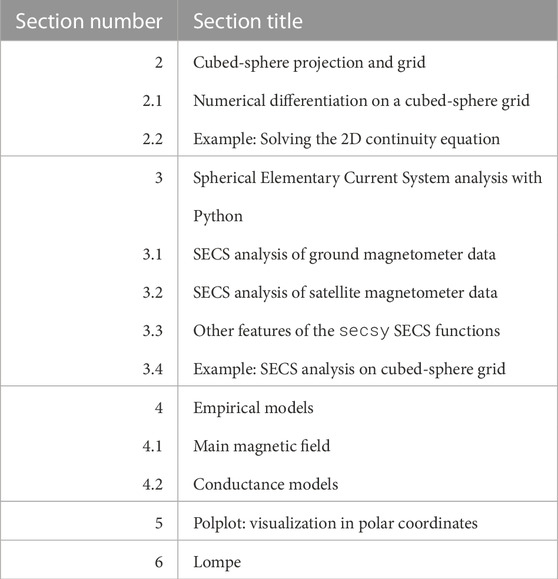
TABLE 1. Overview of the sections describing the Lompe code.

2 Cubed-sphere projection and grid

The basis of the numerical implementations in Lompe is a grid in the cubed-sphere projection (Ronchi et al., 1996). The ionosphere is modeled as a two-dimensional spherical shell at radius R_I (in this paper we use R_E+110 km, where R_E is the mean Earth radius), and the cubed-sphere projection maps every point of the sphere onto a circumscribed cube by extending the line that connects the center of the Earth and the position on the sphere until it intersects the cube. A significant advantage of an analysis grid in the cubed-sphere projection is that regular grids become free of any singularity, avoiding the numerical difficulties of the poles that are present when using spherical polar coordinates (often referred to as the “pole problem”). In addition, regular grids are almost equal area in the cubed-sphere projection.

Cubed-sphere projections and grids are handled in the cubedsphere script, a part of the secsy module. The purpose of the module is to facilitate regional data analyses such as Lompe, and, as we will demonstrate, it can also be used for solving certain partial differential equations on a sphere. The module implements a cubed-sphere projection (CSprojection class) on one face of a cube that has an orientation with respect to the sphere that the user specifies. A regular grid (CSgrid class), centered at the touch point between the surface and the sphere, can be set up to cover a region of interest. The grid resolution can be specified in each direction. With the current implementation, the grid is not intended for global analyses since only one cube face is used. The projection is illustrated in Figure 1A. The figure shows a cross-section of the cube face intersecting a sphere with radius R_I. The grid is equally spaced in angular coordinates (ξ and η, following the notation in Ronchi et al., 1996). Regular grid cells in ξ, η coordinates are projected to increasingly larger cells on the cube face (Figure 1A) and increasingly smaller cells on the sphere as the distance from the intersection point between the cube face and the sphere increases. However, as seen in Figure 1B, the variation in grid cell area on the sphere is small compared to a regular grid in spherical coordinates. The grid projected on the sphere is non-orthogonal. The non-orthogonality is taken into account in all conversions and calculations performed with cubedsphere.

FIGURE 1

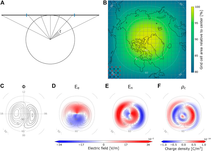
FIGURE 1. Example use of cubedsphere. (A) Cross-section of a cube face (bold black line) tangent to a sphere with radius R_I. In this plane, ξ appears as a polar angle and η as azimuth angle; in the perpendicular plane the roles are reversed. Blue markers show the extent of the example grid in panel (B). (B) An example cubed-sphere grid centered at the north geomagnetic pole. The black dots in the lower left corner represent grid cell center points (the lat, lon, xi, and eta variables in the CSgrid class), and the red dots represent grid cell corners (specified in class variables lat_mesh, lon_mesh, etc.,). The color shading shows the relative area of the grid cells. Coastlines are plotted in the cubed-sphere projection. (C) Electric potential contours from the Weimer (2005a,b) model interpolated on the cubed-sphere grid. (D) Colors show the eastward electric field described by the Weimer potential (gray contour). (E) Same as panel D, but for the northward electric field. (F) Charge density calculated from the divergence of the electric field shown in panels (D,E). The quantities in panels (D–F) are calculated with the finite element differentiation matrices of CSgrid. Note that the differentiation is performed with a higher resolution grid than what is shown in panels (A,B), which is down-scaled for illustration purposes. Panels (C–F) use cubed-sphere projections, oriented such that noon magnetic local time is on top and midnight at bottom [indicated in panel (C)].

The flexibility in choosing the cube’s orientation makes it easy to set up rectangular grids that cover a specific region. For example, in the Observing System Simulation Experiment (OSSE) presented by Laundal et al. (2021), cubed-sphere grids were aligned with simulated satellite tracks for the upcoming Electrojet Zeeman Imaging Explorer (EZIE) mission (Yee et al., 2021). The three EZIE satellites will use the Zeeman effect to give multi-point magnetic field measurements at $\sim 85$ km altitude. These measurements will be interpolated to a 2D image of the electrojet by using spherical elementary currents on a cubed-sphere grid. In Section 3, we discuss how to use the secsy module for such analyses.

2.1 Numerical differentiation on a cubed-sphere grid

The CSgrid class facilitates numerical differentiation of functions that are defined on the grid. The CSgrid.get_Le_Ln() function returns two N × N matrices, ${\mathbb{D}}_{\mathbf{e}\cdot \nabla }$ and ${\mathbb{D}}_{\mathbf{n}\cdot \nabla }$, where N is the number of grid cells. The matrices yield the eastward and northward components of the gradient of a scalar field that is defined on the N cells of the CSgrid object, respectively. That is, the matrix elements are defined by the combination of the finite central difference scheme for differentiation in ξ, η coordinates, the conversion between cubed-sphere coordinates and spherical coordinates, and the orientation and position of the cube face with respect to the underlying global coordinate system (for the example in Figure 1, we use centered dipole coordinates). The conversions between cubed-sphere and spherical coordinates are given by Ronchi et al. (1996) and take the non-orthogonality of the projected coordinates into account. Forward/backward difference schemes are used near the edges, and the size of the stencil used to calculate the elements of the differentiation matrices can be chosen by the user. These differentiation matrices can, for example, be applied to a steady-state electric potential Φ to yield the ionospheric electric field, E = −∇Φ. To illustrate this capability, we use an electric potential from the empirical Weimer (2005a), Weimer (2005b) model, with solar wind velocity 350 km/s, IMF B_y = 0 nT, B_z = −4 nT, solar wind density 2 particles per cm³, and dipole tilt angle 25° (referred to as the “Weimer potential” for the rest of the paper). With the Weimer potential interpolated to a cubed-sphere grid, the electric field can be calculated as

$\begin{array}{ll}\hfill {\underline{E}}_e& =-{\mathbb{D}}_{\mathbf{e}\cdot \nabla }\underline{\mathrm{\Phi }},\hfill \\ \hfill {\underline{E}}_n& =-{\mathbb{D}}_{\mathbf{n}\cdot \nabla }\underline{\mathrm{\Phi }},\hfill \end{array}(1)$

where $\underline{\mathrm{\Phi }}$, ${\underline{E}}_e$, and ${\underline{E}}_n$ are column vectors containing elements corresponding to the N cells in the CSgrid; the Weimer potential, the eastward component of the electric field, and the northward component of the electric field, respectively. We use the underline to indicate column vectors that represent a set of scalar field values throughout the paper. Figure 1C shows the Weimer potential in the grid projection, while the derived eastward and northward components of the electric field are shown in panels D and E.

The divergence of a vector field defined on the N cells in the CSgrid can be found using the N × 2N matrix ${\mathbb{D}}_{\nabla \cdot }$ returned from CSgrid.divergence(). This divergence matrix is also implemented using a finite difference scheme. It operates on a 2N element column vector comprised of the eastward and northward components of a vector field defined on the grid and stacked on top of each other. For example, Gauss’ law says that the electric charge is ρ_c = ϵ₀∇ ⋅E, which means that we can use the set of vector components found above, ${\underline{E}}_e$ and ${\underline{E}}_n$, to calculate the electric charge density associated with the Weimer potential in every grid cell

${\underline{\rho }}_c={ϵ}_0{\mathbb{D}}_{\nabla \cdot }\left(\begin{array}{c}\hfill {\underline{E}}_e\hfill \\ \hfill {\underline{E}}_n\hfill \end{array}\right),(2)$

Assuming that the radial derivative of the electric field is zero. ϵ₀ is the vacuum permittivity. The charge density is shown in Figure 1F.

There are also methods in the CSgrid class that can be useful for working with observational data on cubed-sphere grids. Given the observation locations, ingrid() can be used to check if observations are located within the grid. The indices of the grid cells in which the observations are located can be found using bin_number(). There is also a possibility to use count() to obtain the total number of observations within each grid cell.

2.2 Example: Solving the 2D continuity equation

The differentiation matrices in CSgrid can be used to solve certain partial differential equations. In this section, we show an example where they are used to solve the 2D steady-state continuity equation on a domain covered by a CSgrid object. We want to find the resulting distribution of plasma density, n, given a plasma production function, P, a 2D velocity field specified by v_e and v_n, and a plasma decay factor β. For an incompressible plasma, we have that

$\mathbf{v}\cdot \nabla n=P-\beta n.(3)$

With P, v_e, v_n and n defined on each cell of a CSgrid, Eq. 3 can be written as a matrix equation,

$\left[\mathrm{diag}\left({\underline{v}}_e\right){\mathbb{D}}_{\mathbf{e}\cdot \nabla }+\mathrm{diag}\left({\underline{v}}_n\right){\mathbb{D}}_{\mathbf{n}\cdot \nabla }+\beta \mathbb{I}\right]\underline{n}=\underline{P}.(4)$

The differentiation matrices ${\mathbb{D}}_{\mathbf{e}\cdot \nabla }$ and ${\mathbb{D}}_{\mathbf{n}\cdot \nabla }$ can be returned as scipy.sparse matrices, which is useful in applications like this, since most of the elements are zero. $\mathbb{I}$ is the N × N identity matrix. Solving the continuity equation is now only a matter of inverting the matrix in square brackets in Eq. 4.

An example production function P and velocity field v are shown in the left panel of Figure 2. In this example P represents solar EUV ionization in proportion to cos(χ) (Ieda et al., 2014), where χ is the solar zenith angle, and the subsolar point is located at 10° latitude and noon local time (up in the figure). In Figure 2 the production function is normalized as P/P₀, where P₀ is the plasma production rate at the subsolar point. The velocity field is based on the Weimer potential. It is shown as vectors and as contours of constant electric potential, Φ, where −∇Φ = −v ×B. We assume a dipole magnetic field with mean magnetic field B₀ = 30 μT. In this example, we have transformed the electric potential and velocity field to an inertial frame by adding co-rotation (Laundal et al., 2022b). The decay factor, β, is set to 1/(3 h), i.e., the plasma decay factor is such that it takes 3 h for the plasma to decay by factor 1/e.

FIGURE 2

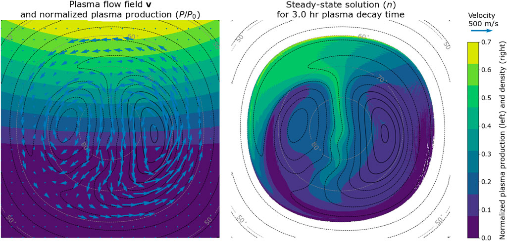
FIGURE 2. Left: Normalized plasma production P (colors), electric potential (black contours), and resulting velocity field v (above 60° latitude, blue arrows). Right: Normalized steady-state solution for the plasma density n (colors) assuming a 3-h plasma decay time, and electric potential (black contours).

The solution plasma density, n, is shown to the right in Figure 2. Like the production function, the density is also normalized, by dividing by P₀/β, which is the solution to Eq. 3 at the subsolar point, where ∇n = 0. The inversion of the matrix in square brackets in Eq. 4 gives meaningful results only within closed convection contours, within which the boundary value problem is well defined. We therefore mask densities equatorward of 60° latitude, where co-rotation dominates. We see that poleward of 60°, the density pattern has features that are well known from studies of the long-lived F-region plasma: A tongue of ionization in the central region, due to anti-sunward transport of plasma produced at lower latitudes, and a mid-latitude trough in the dusk return flow region (Kelley, 2009).

3 Spherical elementary current system analysis with Python

The secsy module contains functions which facilitate SECS analyses. SECS are basis functions that were originally used for regional analyses of ionospheric current systems (Amm, 1997). They can be used as alternatives to spherical harmonics when the focus is on localized regions rather than global patterns. There are two types of SECS, describing divergence-free and curl-free vector fields on a spherical shell. Both divergence-free and curl-free basis functions describe a global 2D vector field that decreases in amplitude as 1/tan (θ/2), where θ is the polar angular distance from the basis function’s “pole”. This functional form implies that the amplitudes fall off rapidly; each basis function has a short range even though they are, in principle, global. According to Vanhamäki and Amm (2011) and the Helmholtz theorem, by placing the SECS basis functions sufficiently close and choosing their amplitudes appropriately, their sum can represent any well-behaved 2D vector field on a spherical shell.

3.1 SECS analysis of ground magnetometer data

So far, SECS have primarily been used for analyses of ground magnetometer data. Given a set of simultaneous measurements from ground magnetometer stations, divergence-free SECS can be used to estimate an equivalent overhead current sheet density, and a corresponding magnetic field everywhere within the analysis region. The divergence-free equivalent current J° at radius R_I, is represented with SECS as

$\mathbf{J}°\left(\mathbf{r}\right)=\sum _i\frac{S_i^{°}}{4\pi R_I}\cot \left(\frac{{\theta }_i}{2}\right){\widehat{\mathbf{e}}}_i,(5)$

where θ_i is the colatitude of the location r in a coordinate system where the location of the ith SECS basis function defines the north pole, and ${\widehat{\mathbf{e}}}_i$ is an eastward unit vector in that coordinate system. $S_i^{°}$ represents the amplitude of the ith SECS basis function. As in Laundal et al. (2022c), the superscript ° signifies “divergence-free”.

The secsy module contains functions that calculate matrices that relate a set of divergence-free SECS amplitudes, $S_i^{°}$, to the corresponding divergence-free current at any given set of coordinates on the spherical shell (get_SECS_J_G_matrices()). In addition, get_SECS_B_G_matrices() returns matrices that relate SECS amplitudes to corresponding magnetic field perturbations at any given set of coordinates at any altitude. This function uses the analytical expressions derived by Amm and Viljanen (1999). Together, these two functions can be used to calculate a map of the equivalent current through the following steps:

1. Get design matrix ${\mathbb{H}}_g°$ that relates a set of measured magnetic field components $\mathrm{\Delta }{\underline{B}}_g$ to a set of divergence-free SECS amplitudes $\underline{S}°$ (containing the amplitudes $S_i^{°}$) from get_SECS_B_G_matrices().

2. Solve the inverse problem $\mathrm{\Delta }{\underline{B}}_g={\mathbb{H}}_g°\underline{S}°$ for $\underline{S}°$

3. Get design matrix $\mathbb{J}°$ that relates a set of divergence-free current densities, $\underline{J}°$, to $\underline{S}°$ from get_SECS_J_G_matrices().

4. Calculate the current densities as $\underline{J}°=\mathbb{J}°\underline{S}°$.

If the task is to interpolate magnetometer measurements, $\mathbb{J}°$ in the last two steps can be replaced with a different ${\mathbb{H}}_g°$ matrix, that relates the amplitudes $\underline{S}°$ to the magnetic field at the interpolation points.

The above procedure focuses on ground magnetometers, but the get_SECS_B_matrices() function accepts evaluation points at any radius. It can thus also be used in analyses of magnetometer data from higher altitudes; below the ionospheric current layer at R_I, for example with data from the upcoming EZIE mission (Laundal et al., 2021), or above the current layer, for example with data from low-flying satellites like Swarm or CHAMP (Laundal et al., 2016).

Note that get_SECS_B_matrices() and get_SECS_J_matrices() return multiple matrices, one for each vector component, instead of the single matrix in this example. The component matrices can be stacked vertically to form a single composite matrix that calculates all the desired vector components. Note also that the functions accept NumPy arrays as input and that all calculations are vectorized and therefore fast.

3.2 SECS analysis of satellite magnetometer data

The above example assumes that only the divergence-free part of the horizontal ionospheric current contributes to the observed magnetic field. This is true for ground observations; according to the Fukushima theorem, the magnetic fields of field-aligned currents and associated horizontal curl-free currents cancel below the ionosphere in polar regions where the main magnetic field is approximately radial (Fukushima, 1994). In space, above the horizontal current, we must include the curl-free current system in the analysis. The curl-free current can be represented with SECS as

${\mathbf{J}}^{\star }\left(\mathbf{r}\right)=\sum _i\frac{-S_i^{\star }}{4\pi R_I}\cot \left(\frac{{\theta }_i}{2}\right){\widehat{\mathbf{n}}}_i,(6)$

where the superscript ^⋆ signifies “curl-free”, and ${\widehat{\mathbf{n}}}_i$ is a northward unit vector in a coordinate system that has the ith SECS basis function in the north pole. The get_SECS_J_G_matrices() and get_SECS_B_G_matrices() functions can be used with curl-free currents in the same way as for divergence-free currents, except that the current_type keyword should be set to “curl_free” instead of “divergence_free”. The curl-free amplitudes, $S_i^{\star }$, can be thought of as electric line currents that flow down to or up from the spherical shell at radius R_I, extending to infinity. Therefore, its unit is Ampere. The corresponding horizontal curl-free current [Ampere per meter] distributes this current across the globe, with a uniform radial divergence with the opposite sign as $S_i^{\star }$, ensuring current continuity (Amm, 1997).

3.3 Other features of the secsy SECS functions

The SECS functions in secsy also support a number of features that are often useful in SECS analysis.

The SECS basis functions are infinite at θ_i = 0, which can cause numerical problems. To avoid this, a modification is often applied poleward of some limit θ₀. This modification, described in detail by Vanhamäki and Juusola (2020), can be applied with the SECS functions by specifying θ₀ with the singularity_limit keyword. Note that the singularity modification is applied to both types of currents but not to the magnetic field of the divergence-free current. The reason is that the magnetic field of the modified J° likely does not have an analytic expression, and that the modification would be minimal since the ground magnetic field is usually evaluated at radii where the effect of the singularity is greatly reduced (Vanhamäki and Juusola, 2020).

Magnetic disturbances observed with ground magnetometers are not only associated with currents in space, but also with induced currents in the conducting Earth. The magnetic field of ground-induced currents can be taken into account in SECS analyses in at least two ways: (i) They can be modeled directly, in the same way as ionospheric currents, by placing divergence-free SECS poles at some radius below ground, or (ii) they can be modeled as so-called image currents. The image current method assumes that there is a super-conducting layer in the Earth’s interior that exactly cancels the radial magnetic field of the ionospheric currents at some radius R_C. Juusola et al. (2016) showed how the magnitudes of the image currents relate to the corresponding ionospheric currents. The effect of the image current is to change the radial dependence of the magnetic field, and this can be included in secsy SECS analyses by specifying R_C through the induction_nullification_radius in calls to get_SECS_B_G_matrices(). An advantage of the image current method is that it does not add any degrees of freedom to the SECS model since the image current amplitudes are given by the ionospheric current amplitudes. A disadvantage is that it does not account for the effects of finite and non-uniform ground conductivities.

The curl-free SECS basis functions can–since they have zero curl–be written as gradients of scalar fields (potentials). That is, Eq. 6 can be written as

$\begin{array}{ll}\hfill {\mathbf{J}}^{\star }& =\sum _i\frac{-S_i^{\star }}{4\pi R_I}\cot \left(\frac{{\theta }_i}{2}\right){\widehat{\mathbf{n}}}_i=\nabla V\hfill \\ \hfill & =\nabla \left[\sum _i\frac{-S_i^{\star }}{2\pi }\ln \left(\sin \left(\frac{{\theta }_i}{2}\right)\right)\right].\hfill \end{array}(7)$

The scalar potential representation can be useful in studies of ionospheric convection electric fields, assuming that Faraday’s law can be set equal to zero. Reistad et al. (2019) used SuperDARN (Chisham et al., 2007) line-of-sight measurements of ionospheric convection to constrain curl-free SECS representations of convection electric fields and visualized the result by plotting equipotential contours. The same approach is used in the Lompe technique (Laundal et al., 2022c). The corresponding curl-free SECS amplitudes can be interpreted in terms of electric charges: Each basis function represents a line that extends from the base of the ionosphere to infinity, and the amplitude is equal to the electric line charge density. The potential representation on the right hand side of Eq. 7 can be calculated with the matrix returned by get_SECS_J_G_matrices() with the $\mathtt{c}\mathtt{u}\mathtt{r}\mathtt{r}\mathtt{e}\mathtt{n}\mathtt{t}\text{\_}\mathtt{t}\mathtt{y}\mathtt{p}\mathtt{e}$ keyword set to “potential”.

3.4 Example: SECS analysis on cubed-sphere grid

In this section, we show an example where secsy design matrix functions and cubed-sphere grids are used to estimate magnetic perturbations on ground given the Weimer potential, and an assumption of constant ionospheric conductances. Without gradients in the Pedersen or Hall conductances, the divergence of the height-integrated ionospheric Ohm’s law reduces to

$j_{\Vert }={\mathrm{\Sigma }}_P\nabla \cdot \mathbf{E},(8)$

where Σ_P is the Pedersen conductance, j_‖ is the field-aligned current density, and E is the ionospheric electric field.

Consider a set of curl-free SECS poles in the center of the cells of the cubed-sphere grid in Figure 1B. The curl-free amplitude in the ith grid cell, $S_i^{\star }$, represents an electric line current flowing into or out of the spherical shell at radius R_I, i.e., the total field-aligned current integrated over the cell. In Section 2, we obtained the divergence of the Weimer ionospheric electric field defined on the grid cells (Figure 1F shows this quantity multiplied by ϵ₀). The corresponding FAC densities can be found through Eq. 8 if Σ_P is known. Then $S_i^{\star }$ can be found directly through multiplication with the grid-cell area, A_i,

$S_i^{\star }=j_{\Vert ,i}{A}_i.(9)$

Recall that only the divergence-free part of the horizontal ionospheric current, J°, contributes to the observed magnetic field on ground, and the divergence-free SECS amplitudes, $S_i^{°}$, that scale J° must be found. With no conductance gradients and a constant Hall-to-Pedersen conductance ratio α = Σ_H/Σ_P = 1, the curl-free and divergence-free SECS amplitudes are related as (Amm et al., 2002; Juusola et al., 2009)

$S_i^{°}=-S_i^{\star }.(10)$

By assuming that both the Hall and Pedersen conductances are 10 mho across the grid, we get a vector $\underline{S}°$ containing the divergence-free SECS amplitudes for all cells on the grid. The corresponding magnetic perturbations for a set of locations on ground, $\mathrm{\Delta }{\underline{B}}_g$, can be calculated as

$\mathrm{\Delta }{\underline{B}}_g={\mathbb{H}}_g^{°}\underline{S}°,(11)$

where ${\mathbb{H}}_g^{°}$ is the matrix that relates the SECS amplitudes (S_i°, contained in ${\underline{S}}^{°}$) to ground magnetic field vector components. The function get_SECS_B_G_matrices() calculates ${\mathbb{H}}_g^{°}$ given the coordinates and radii of the evaluation locations, and the coordinates of the SECS poles, in this case the centers of the cells in our cubed-sphere grid. In this example, the evaluation locations are at radius R_E and are set to the corners of the grid cells. The magnetic disturbance on ground is shown in Figure 3. The horizontal magnetic field is shown as black arrows, while the upward magnetic field is shown with colors. The gray contours represent the Weimer potential.

FIGURE 3

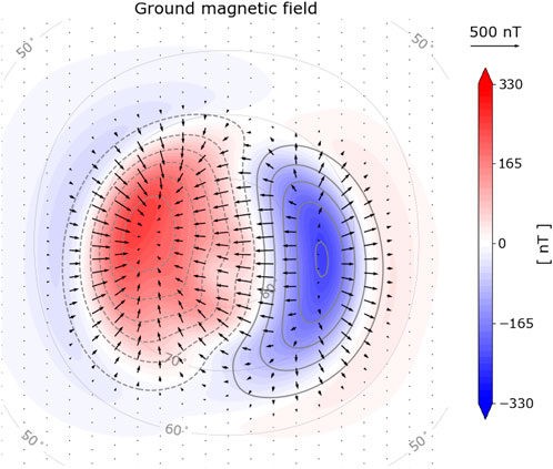
FIGURE 3. Example of how the secsy module can be used to relate an ionospheric electric potential to magnetic field disturbances on ground in the polar region, assuming uniform ionospheric conductance. Results are shown in the cubed-sphere projection. The black arrows represent the horizontal components of the magnetic field disturbance, and color contours represent the upward magnetic field disturbance. The gray contours represent the Weimer ionospheric electric potential used throughout this paper.

The Lompe technique uses the same approach as above except that the conductances are not assumed to be uniform. In Lompe, the full expressions for the divergence and curl of the ionospheric Ohm’s law are taken into account by using the CSgrid differentiation matrices that were introduced in Section 2.

4 Empirical models

In the Lompe technique, magnetic and electric fields are related through the ionospheric Ohm’s law, and the electric field and F-region ion velocity are related through the generalized Ohm’s law. The ionospheric Ohm’s law involves ionospheric conductances, and both equations involve the main magnetic field of the Earth. The Lompe code includes modules to estimate these quantities, discussed briefly in this section.

4.1 Main magnetic field

The International Geomagnetic Reference Field (IGRF) is a standard model of the Earth’s magnetic field, maintained by the International Association of Geomagnetism and Aeronomy (IAGA). The IGRF model represents the magnetic field as a set of spherical harmonics, with a new set of coefficients every 5 years to account for temporal changes. Linear interpolation of the model coefficients is used between versions. The most recent version was presented by Alken et al. (2021). The Lompe technique requires magnetic field values on every grid point. When the grid is defined in geographic coordinates (default), IGRF magnetic field values are calculated with the ppigrf module (Laundal, 2022), which is a pure-Python implementation of the IGRF that gives IGRF model predictions given position and date. The position can be specified in either geodetic or geocentric coordinates. While other Python modules that calculate IGRF values exist, many of them are wrappers of Fortran code, which can be tricky to compile. Despite being a pure-Python implementation, the IGRF calculations are quite fast since ppigrf is fully vectorized.

For some applications IGRF is not the appropriate model. For example, in this paper our examples are based on the statistical Weimer (2005a), Weimer (2005b) model of electric potential, which is given in magnetic latitude and local time. Since longitude information is missing, it is more appropriate to use a dipole magnetic field, since it is symmetric about the dipole axis. To accommodate such cases, the Lompe code includes an option to use dipole coordinates. This is accomplished using another submodule to Lompe, dipole, which contains functions to calculate dipole magnetic field values, and to convert between geocentric and dipole coordinates. The dipole module also contains functions to convert between magnetic local time and magnetic longitude using Equation (93) of Laundal and Richmond (2017). The dipole module uses the ppigrf module to extract the first three spherical harmonic coefficients, which defines the centered dipole, for any given epoch covered by the IGRF.

4.2 Conductance models

The interpretation of ground magnetometer data in terms of high latitude ionospheric convection requires knowledge about ionospheric conductances, the height-integrated conductivities (e.g., Kamide et al., 1981). The ionospheric conductance depends primarily on the ionization by solar EUV radiation and the contribution to ionization from precipitating particles (auroral conductance). The Lompe code also contains functions for calculating the solar EUV conductances and the auroral conductances from the Hardy et al. (1987) empirical model.

A novel method for calculating the solar EUV conductance, Σ_EUV, is implemented in the EUV_conductance() function. The method uses a modified version of the empirical model from Moen and Brekke (1993) where cos(χ) is replaced with a function q′(χ) that specifies the relative maximum production due to solar EUV assuming a radially stratified atmosphere, with χ the solar zenith angle. The full technique is explained in Section 2.4 in Laundal et al. (2022c). This adjustment gives EUV conductances without infinite gradients at the sunlight terminator. The Hall and Pedersen conductances are calculated given a solar radio flux index, F_10.7, and a set of solar zenith angles corresponding to the locations of interest. Functions in the sunlight module can be used to calculate χ. Σ_EUV is by default scaled to coincide with the empirical model by Moen and Brekke (1993) at low solar zenith angles (other empirical models can be chosen using the calibration keyword).

For auroral conductances, Σ_auroral, the hardy() function is an implementation of the Hardy et al. (1987) model, which is based on satellite observations of precipitating particles. Given a Kp index and coordinates in magnetic latitude and local time, the method returns empirical Hall and Pedersen conductances. It is difficult to know the auroral conductances precisely, mainly because of the high variability in the auroral precipitation. The Hardy et al. (1987) model function is only meant to be a rough estimate in applications of the Lompe technique. If possible, better auroral conductance estimates should be obtained from observations such as auroral images.

The hardy_EUV() function combines the implementations for solar and auroral conductance contributions and returns the total conductances given a set of coordinates. In the latest version of the Lompe code (v1.1), the total conductances are calculated using the vector sum of the solar EUV and auroral contributions, ${\mathrm{\Sigma }}_{\text{total}}=\sqrt{{\mathrm{\Sigma }}_{\text{EUV}}^2+{\mathrm{\Sigma }}_{\text{auroral}}^2}$ (Robinson et al., 2020). Example output from the conductance function is shown in Figure 4, where the Hall conductance (left) and Pedersen conductance (right) are plotted for a region poleward of 50° magnetic latitude. The solar zenith angles are calculated for 2 July, and the auroral conductances are patterns for Kp 4.

FIGURE 4

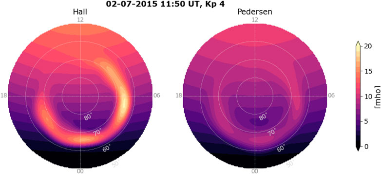
FIGURE 4. Example Hall and Pedersen conductances where solar conductances are like on 2 July, and auroral conductances are Hardy et al. (1987) model patterns for Kp 4. The axes have magnetic latitude and local time (centered dipole) coordinates, and show a region poleward of 50° magnetic latitude. Magnetic noon is up.

5 Polplot: Visualization in polar coordinates

The polplot module, which is included as a submodule to Lompe, is useful for visualizing data in a polar coordinate system, specifically a latitude and local time grid. Given a Matplotlib axis object, an object of the Polarplot class returns a polar axis centered at the pole, where noon is at the top and dusk to the left. Most Polarplot plotting functions are equivalent to the corresponding Matplotlib function, and keyword arguments accepted by pyplot functions (such as color, linewidth, zorder, etc.,) can also be given to the Polarplot functions. For example, polplot was used when making Figure 4, where Polarplot.contourf() made the filled contours representing the ionospheric conductances in a magnetic latitude and local time system.

Figure 5 shows examples of data visualization in polar coordinates and in a cubed-sphere projection. Coordinates are given in magnetic latitude and local time for the polar axes (left). In the plot to the right, the grid ξ, η coordinates are treated as Cartesian coordinates on the Matplotlib axes. An orange X marks the Geographic North Pole. Black rectangles on the polar axes show the extent of a cubed-sphere grid covering much of North America and Greenland. The bold grid edge corresponds to the lower edge of the grid. The pairs of panels in the two rows show the same grids. The gray meshes in the top row panels represent the grid cells. Coastlines, converted to magnetic apex coordinates, are added to the polar axis using the coastlines() function. The cubed-sphere projection class has a function called get_projected_coastlines() that returns coastlines projected to cubed-sphere ξ, η coordinates. The gray line in both panels marks the sunlight terminator as it is on 10 March at midnight UT. Regions where the solar zenith angle is more than 90° are shaded gray using the plot_terminator() function, which also adds the location of the terminator to the polar axis. The bottom row panels show the Weimer potential as black contours. Blue arrows show the E × B convection velocity resulting from the electric field described by the Weimer potential in a co-rotating frame.

FIGURE 5

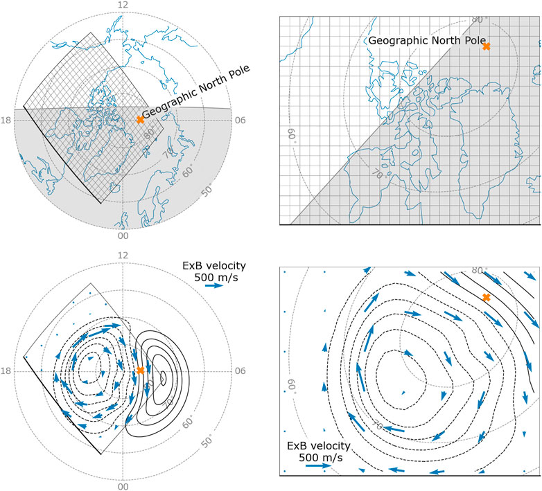
FIGURE 5. Example of different representations of data on Polarplot polar axes (left), and Cartesian axes (right). The left panels have coordinates in magnetic latitude and local time, and show a region poleward of 50° magnetic latitude. The black frames show the extent of the grid in the right panels. The bold edge corresponds to the lower edge of the grid projections. The right panels show data in the cubed-sphere projection. The cubed-sphere grid is 7,000 × 5,000 km defined on a cube face centered at 88°W and 72°N and rotated 45°. The gray mesh in the top panels is the grid, where each cell is 200 × 200 km. In the top panels, coastlines are shown in blue, and regions where the solar zenith angle is $\ge 90°$ (sunlight terminator) are shaded gray. The black contours in the bottom panels represent the ionospheric electric potential. The blue arrows represent the E ×B convection velocities. An orange X represents the Geographic North Pole in all panels.

6 Lompe

In this section we demonstrate the full Lompe technique, which combines the modules from the previous sections. The Lompe technique (Laundal et al., 2022c) is implemented in the model module. The technique relates vector components of ionospheric convection electric fields, $\underline{E}$, F-region plasma convection velocities, $\underline{v}$, ground magnetic field disturbances, ${\underline{B}}_g$, and space magnetic field disturbances, ${\underline{B}}_s$, to a model vector $\underline{m}$ through a set of linear equations

$\left(\begin{array}{c}\hfill \underline{E}\hfill \\ \hfill \underline{v}\hfill \\ \hfill {\underline{B}}_g\hfill \\ \hfill {\underline{B}}_s\hfill \end{array}\right)=\underline{y}=\left(\begin{array}{c}\hfill \mathbb{E}\hfill \\ \hfill \mathbb{V}\hfill \\ \hfill {\mathbb{B}}_g\hfill \\ \hfill {\mathbb{B}}_s\hfill \end{array}\right)\underline{m}=\mathbb{G}\underline{m}.(12)$

In Lompe, the model vector, $\underline{m}$, contains the amplitudes of the curl-free SECS basis functions representing the convection electric field. The different block matrices relate different quantities to the model vector $\underline{m}$: $\mathbb{E}$ relates electric field vector components to $\underline{m}$ through Eq. 6, $\mathbb{V}$ relates F-region plasma velocity components to $\underline{m}$ by assuming that the electric field and plasma are frozen-in, ${\mathbb{B}}_g$ and ${\mathbb{B}}_s$ relate magnetic field vector components below (subscript g) and above (subscript s) the ionosphere to $\underline{m}$ by using the ionospheric Ohm’s law. Use of the ionospheric Ohm’s law requires that conductances are known. The conductance determines both a scale factor–how strong the electric fields have to be in order to explain the observed magnetic field–and the distribution of the electric field. If magnetic field measurements are used in the inversion, it is therefore highly recommended to use Lompe in cases when the conductances are precisely known. The Lompe conductance module (Section 4.2) includes functions that yield precise estimates of solar EUV-induced conductance, but auroral conductance should preferably come from measurements. The total design matrix $\mathbb{G}$ thus depends on ionospheric conductances, the choice of grid, and the coordinates of the model predictions, $\underline{y}$. For a thorough description of how $\mathbb{G}$ is calculated, see Section 3.2 in Laundal et al. (2022c).

Figure 6 gives an overview of the various steps to carry out a Lompe inversion. The first step is setting up a cubed-sphere grid that covers the region we want to model. The location, orientation, size, and resolution of the grid should be adapted to the input data coverage. In addition, functions for calculating the Hall and Pedersen conductances are required. The Lompe Emodel is then initialized given the grid and conductance functions. Emodel assumes all input in geographic coordinates by default, but the dipole keyword can be used to make all calculations in centered dipole coordinates, and with a centered dipole magnetic field instead of the IGRF (see Section 4.1).

FIGURE 6

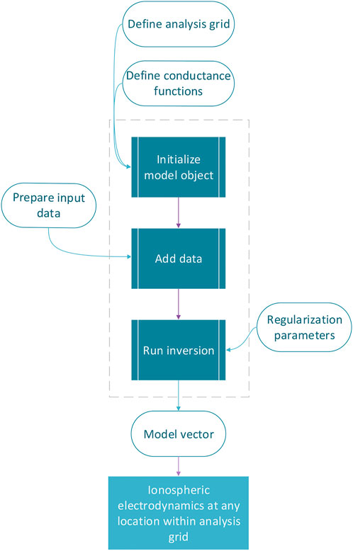
FIGURE 6. Flow chart showing the basics steps in the Lompe workflow.

The next step is to add the input data ($\underline{y}$ in the equation above). The input data to a Lompe Emodel must be an object of the Data class, which contains the data values (vector components) and coordinates. To help set up a Data object, the Lompe package includes a stand-alone module called dataloader. It contains functions that work with convection data from DMSP satellites (Rich, 1994) (from the CEDAR Madrigal database), the SuperMAG network of magnetometers (Gjerloev, 2012), the network of SuperDARN radars (Chisham et al., 2007), and AMPERE’s Iridium magnetometer data (Waters et al., 2020).

When initializing Data objects, the measurements go through sanity checks that ensure the input data is of the correct shape and with valid values, and NaNs are removed from the data set. All data should be given in SI-units. Coordinates and components should be given in geographic coordinates, unless the Emodel object is initialized with the dipole keyword. If not all vector components are known, the components parameter can be used to indicate which of the eastward, northward, and upward components are included in the data set. For convection and electric field data, a line of sight can be specified.

The Data initialization requires specification of the type of measurement. The datatype categories are: magnetometer observations from ground (“ground_mag”), magnetometer observations from space associated only with field-aligned currents (“space_mag_fac”), “full” magnetometer observations from space (“space_mag_full”), “convection” data, and ionospheric convection electric field (“Efield”). In addition, there is an option to use field-aligned current density (“fac”) as input data, which can be useful for studies of, e.g., magnetosphere-ionosphere (M-I) coupling.

There are two categories of space magnetometer observations due to different heights and magnetometer precision of satellites that measure magnetic disturbances from space. For example, Iridium magnetic data is dominated by FACs since it is taken at around 800 km altitude and by magnetometers that do not have the precision of science-mission instruments. Low-flying, precise magnetometers (e.g., Swarm and CHAMP) will measure perturbations associated with both field-aligned currents and the horizontal divergence-free currents below the satellite, i.e., the “full” disturbance (Laundal et al., 2016).

The Data objects must contain the typical scale of the measurements. For example, convection data could have typical scales of 100 m/s, while ground magnetic field disturbances are typically on the scale of 100 ⋅ 10^–9 T. The scales contribute to the data covariance matrix (for details, see Section 3.3 in Laundal et al., 2022c), and therefore partly determine the relative weight of the data set in the inversion; by increasing the scale of one dataset while keeping the scale of other datasets fixed, its relative weight in the inversion decreases. Default values are used if the scale is not specified. In addition, the data covariance matrix depends on the error parameter, which specifies the measurement error. While scale is a single value for a whole dataset, error can be specified on a point by point basis. If the error is not given, it is set to zero.

The finished Data objects can be passed to the Lompe Emodel object using the add_data() method. Once all input data is added to the Emodel, the run_inversion() method can be called. This function automatically creates the appropriate design matrix and solves Eq. 12 for $\underline{m}$ using regularized least-squares. Two regularization parameters can be specified in calls to run_inversion(). The regularization encourages relatively smooth solutions, with stronger gradients in the Quasi-Dipole (Richmond, 1995) north-south direction compared to east-west. Therefore this step depends on the apexpy Python module (Emmert et al., 2010; van der Meeren et al., 2021). The regularization represents prior assumptions about the model, and the regularization parameters determine how much weight these assumptions should have relative to the model’s ability to fit the data. Choosing the optimal set of regularization parameters is therefore an important task, which requires some experimentation. Automated methods for choosing regularization parameters, for example based on L-curve analysis (Hansen, 1992), could be included in future updates of the code. The details of the inversion is described in Section 3.3 in Laundal et al. (2022c). The perimeter_width parameter can be used to specify the perimeter around the grid from which observations are included in the inversion. The default is 10, which means observations within a 10 cell wide perimeter around the grid will be included. Measurements from outside the perimeter are ignored. If the Lompe inversion is to be performed for multiple time steps but with the same grid setup, the clear_model() function will reset the Emodel so that the inversion can be performed using new input data.

After the inversion, $\underline{m}$ is known, and ionospheric parameters can be estimated at any location within the analysis region. Emodel methods can return model predictions for the following parameters: convection electric field (E()), electric potential (E_pot()), convection velocity (v()), ground magnetic field disturbances (B_ground()), space magnetic field disturbances (B_space() for “full” disturbance, or B_space_FAC() for disturbance due to FACs only), ionospheric horizontal height-integrated currents (j()), and FACs (FAC()). The predicted ionospheric quantities can also be visualized using the lompeplot() function.

Figure 7 shows an example of a Lompe output, visualized with lompeplot. The analysis grid covers the same area as in Figure 5, and the cell dimension is 100 × 100 km. We use the same conductance maps as in Figure 4, shown in the bottom left panels of Figure 7. The input data is the ionospheric electric field derived from the Weimer potential (Figures 1D, E). We set the regularization parameters in the inversion to λ₁ = 0.02 and λ₂ = 0.01. These values are low since the Weimer electric field can be evaluated everywhere on the grid, with near zero error. With realistic data distributions and uncertainties, the inverse problem is ill-conditioned, and stronger regularization is required. The top left panel shows the predicted convection pattern and electric potential. The magnetic field in space, evaluated 110 km above R_I, is shown as black arrows in the next panel, and the color contours show the vertical current density (FACs). The third panel from the left shows the magnetic field disturbances on ground in the same format as in Figure 3. The panel below shows the horizontal height-integrated ionospheric currents.

FIGURE 7

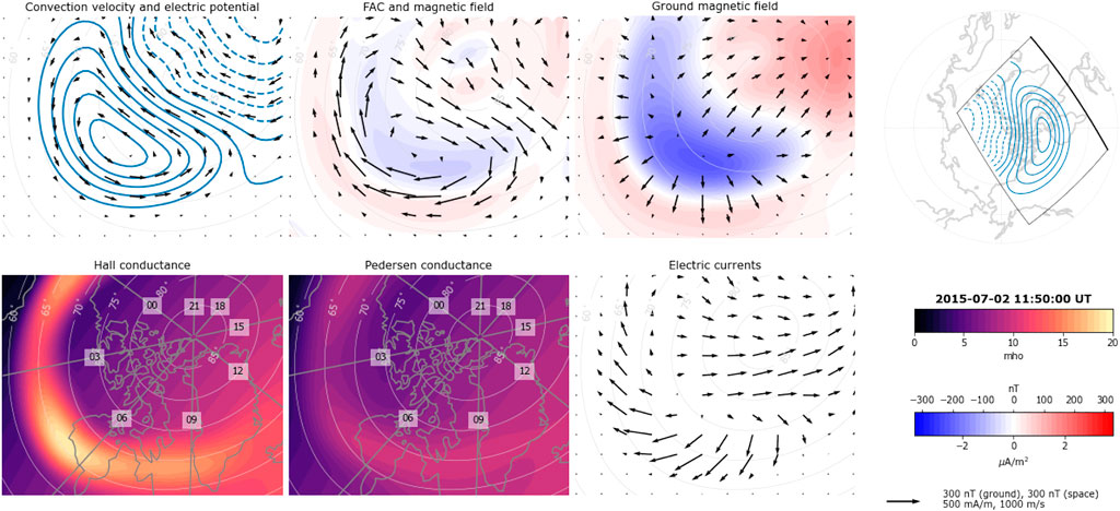
FIGURE 7. Lompe output given synthetic electric field data as input. The model conductances are for 2 July 2015 at 11:50 UT and Kp 4. The top row shows, from left to right: Convection flow field and electric potential contours; horizontal magnetic field disturbances 110 km above the ionosphere as black arrows and radial current density as color contours; horizontal ground magnetic field perturbations as black arrows and radial magnetic field perturbations as color contours; and a map that shows the grid’s position and orientation with respect to apex magnetic latitude and local time. The bold grid edge corresponds to the lower edge of the projections shown in the other plots. The bottom row shows, from left to right: Pedersen conductance; Hall conductance; horizontal height-integrated ionospheric currents based on Lompe output; and color scale/vector scales.

The Lompe technique also offers an alternative way to solve the current continuity equation used in global magnetohydrodynamic (MHD) simulations to couple the magnetosphere and the ionosphere (e.g., Wiltberger et al., 2004; Merkin and Lyon, 2010). The ionospheric boundary condition in MHD models is specified by using the ionospheric Ohm’s law to solve for the electric field given a map of field-aligned currents. This can be done in a Lompe inversion by using field aligned currents as data input. Currently fac data points must be given at all grid locations, in contrast to all the other data types which can be specified at arbitrary locations. Figure 8 shows an example of the Lompe technique applied with (synthetic) FAC data obtained from the Average Magnetic field and Polar current System (AMPS) model (Laundal et al., 2018). The AMPS output is for solar wind velocity 350 km/s, IMF B_y = 0 nT, B_z = −4 nT, and dipole tilt angle 25°. Model ionospheric conductances are for 1 August and Kp 4. The analysis region covers a large portion of the high-latitude northern hemisphere, and the grid cell dimension is 80 × 80 km. In this inversion, the regularization parameters are λ₁ = 0.02 and λ₂ = 0.01. This is an example of how Lompe can be used to calculate the electric field, ionospheric convection, horizontal ionospheric currents, and ground magnetic field perturbations implied by given patterns of field-aligned current and ionospheric conductance.

FIGURE 8

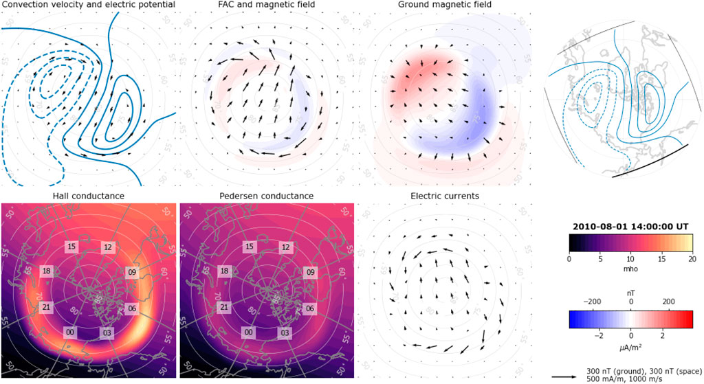
FIGURE 8. Lompe inversion results using synthetic field-aligned current data from the AMPS model as input. Model ionospheric conductances are for sunlight as on 1 August and empirical auroral patterns for Kp 4. The format of this figure is the same as Figure 7.

7 Concluding remarks

The Lompe Python package is available through Zenodo (Laundal et al., 2022a), but we recommend getting the latest version from the stable branch at https://github.com/klaundal/lompe. It depends on the usual scientific Python modules (NumPy, SciPy, Pandas, Matplotlib) and on two geospace-specific modules (apexpy and ppigrf) that can be installed with pip. The optional dataloader helper module also has some other dependencies, depending on which dataset it is used for. The Lompe package itself does currently not include an install script, but lompe can be imported as a module if the repository is placed in the user’s Python module search path. The lompe namespace includes the secsy, dipole, and polplot modules, and the Data and Emodel classes. We recommend running some of the repository’s example notebooks to test that it is set up correctly. In many cases, the example notebooks should be sufficient to use the Lompe technique: One needs only to adapt the grid setup parameters to the region of interest, change the conductance functions and Data objects, and experiment with the regularization.

As demonstrated in this paper, the Lompe Python package is modular, and the different modules can be useful independently of the Lompe technique. Some modules replicate the functionality of already existing Python packages (Burrell et al., 2018), but with some features that we believe are distinctive. ppigrf, for example, is different from most published IGRF Python packages since it is pure Python. polplot is another example; given the prevalence of polar plots in the literature, similar codes must have been implemented numerous times by several researchers, but we are not aware of any other open-source Python module for plotting data on polar local time/latitude grids. Until recently, there were no public code for SECS analysis; hopefully, the secsy module will help to make this technique more accessible. The Lompe Python package is open-source, and we welcome community participation in continuing its development.

Data availability statement

Publicly available datasets were analyzed in this study. This data can be found here: https://github.com/klaundal/lompe.

Author contributions

AH, KL, and JR planned the paper. AH led the work, wrote most of the paper, produced all but one figure, and wrote the accompanying Jupyter notebooks. KL led the Lompe development, wrote parts of the paper, and made Figure 2. All authors contributed to the Lompe code, read and commented on the manuscript.

Funding

The development of the Lompe code was also helped by synergies with the AMPS model development, funded by ESA through the Swarm Data Innovation and Science Cluster (Swarm DISC) within the reference frame of ESA contract 000109587/13/I-NB.

Acknowledgments

We are grateful to Daniel R. Weimer, Virginia Tech, for developing the Weimer 2005 model and for making it available via CCMC. We thank the science team of the NASA Electrojet Zeeman Imaging Explorer (EZIE) mission for fruitful discussions. EZIE is the Heliophysics Science Mission which was selected to study electric currents in Earth’s atmosphere linking aurora to the Earth’s magnetosphere. EZIE will launch no earlier than September 2024. The principal investigator for the mission is Jeng-Hwa (Sam) Yee at the Johns Hopkins University Applied Physics Laboratory in Laurel, Maryland. We also thank the International Space Science Institute in Bern, Switzerland, for hosting the team “Understanding Mesoscale Ionospheric Electrodynamics Using Regional Data Assimilation”.

Conflict of interest

The authors declare that the research was conducted in the absence of any commercial or financial relationships that could be construed as a potential conflict of interest.

Publisher’s note

All claims expressed in this article are solely those of the authors and do not necessarily represent those of their affiliated organizations, or those of the publisher, the editors and the reviewers. Any product that may be evaluated in this article, or claim that may be made by its manufacturer, is not guaranteed or endorsed by the publisher.

References

Alken, P., Thébault, E., Beggan, C. D., Amit, H., Aubert, J., Baerenzung, J., et al. (2021). International geomagnetic reference field: The thirteenth generation. Earth Planets Space 73, 49. doi:10.1186/s40623-020-01288-x

CrossRef Full Text | Google Scholar

AMGeO Collaboration (2019). A collaborative data science platform for the geospace community: Assimilative mapping of geospace observations (AMGeO) v1, 0.0. doi:10.5281/zenodo.3564914Zenodo

CrossRef Full Text

Amm, O., Engebretson, M. J., Hughes, T., Newitt, L., Viljanen, A., and Watermann, J. (2002). A traveling convection vortex event study: Instantaneous ionospheric equivalent currents, estimation of field-aligned currents, and the role of induced currents. J. Geophys. Res. 107, 1334. doi:10.1029/2002JA009472

CrossRef Full Text | Google Scholar

Amm, O. (1997). Ionospheric elementary current systems in spherical coordinates and their application. J. Geomagn. Geoelec. 49, 947–955. doi:10.5636/jgg.49.947

CrossRef Full Text | Google Scholar

Amm, O., and Viljanen, A. (1999). Ionospheric disturbance magnetic field continuation from the ground to the ionosphere using spherical elementary current systems. Earth Planets Space 51, 431–440. doi:10.1186/BF03352247

CrossRef Full Text | Google Scholar

Burrell, A. G., Halford, A., Klenzing, J., Stoneback, R. A., Morley, S. K., Annex, A. M., et al. (2018). Snakes on a spaceship – An overview of Python in heliophysics. J. Geophys. Res. Space Phys. 123, 10384–10402. doi:10.1029/2018JA025877

CrossRef Full Text | Google Scholar

Chisham, G., Lester, M., Milan, S. E., Freeman, M. P., Bristow, W. A., Grocott, A., et al. (2007). A decade of the super dual auroral radar network (SuperDARN): Scientific achievements, new techniques and future directions. Surv. Geophys. 28, 33–109. doi:10.1007/s10712-007-9017-8

CrossRef Full Text | Google Scholar

Emmert, J. T., Richmond, A. D., and Drob, D. P. (2010). A computationally compact representation of Magnetic-Apex and Quasi-Dipole coordinates with smooth base vectors. J. Geophys. Res. 115, A08322. doi:10.1029/2010JA015326

CrossRef Full Text | Google Scholar

Fukushima, N. (1994). Some topics and historical episodes in geomagnetism and aeronomy. J. Geophys. Res. 99, 19113–19142. doi:10.1029/94JA00102

CrossRef Full Text | Google Scholar

Gjerloev, J. W. (2012). The SuperMAG data processing technique. J. Geophys. Res. 117, A09213. doi:10.1029/2012JA017683

CrossRef Full Text | Google Scholar

Hansen, P. C. (1992). Analysis of discrete ill-posed problems by means of the L-curve. SIAM Rev. Soc. Ind. Appl. Math. 34, 561–580. doi:10.1137/1034115

CrossRef Full Text | Google Scholar

Hardy, D. A., Gussenhoven, M. S., Raistrick, R., and McNeil, W. J. (1987). Statistical and functional representations of the pattern of auroral energy flux, number flux, and conductivity. J. Geophys. Res. 92, 12275–12294. doi:10.1029/JA092iA11p12275

CrossRef Full Text | Google Scholar

Ieda, A., Oyama, S., Vanhamäki, H., Fujii, R., Nakamizo, A., Amm, O., et al. (2014). Approximate forms of daytime ionospheric conductance. J. Geophys. Res. Space Phys. 119, 10397–10415. doi:10.1002/2014JA020665

CrossRef Full Text | Google Scholar

Juusola, L., Kauristie, K., Vanhamäki, H., Aikio, A., and van de Kamp, M. (2016). Comparison of auroral ionospheric and field-aligned currents derived from Swarm and ground magnetic field measurements. J. Geophys. Res. Space Phys. 121, 9256–9283. doi:10.1002/2016JA022961

CrossRef Full Text | Google Scholar

Juusola, L., Nakamura, R., Amm, O., and Kauristie, K. (2009). Conjugate ionospheric equivalent currents during bursty bulk flows. J. Geophys. Res. 114, A04313. doi:10.1029/2008JA013908

CrossRef Full Text | Google Scholar

Kamide, Y., Richmond, A. D., and Matsushita, S. (1981). Estimation of ionospheric electric fields, ionospheric currents, and field-aligned currents from ground magnetic records. J. Geophys. Res. 86, 801–813. doi:10.1029/JA086IA02P00801

CrossRef Full Text | Google Scholar

Kelley, M. C. (2009). The Earth’s ionosphere: Plasma Physics and electrodynamics. second edn. Burlington, MA, USA: Academic Press.

Google Scholar

Laundal, K. M., Finlay, C. C., Olsen, N., and Reistad, J. P. (2018). Solar wind and seasonal influence on ionospheric currents from Swarm and CHAMP measurements. J. Geophys. Res. Space Phys. 123, 4402–4429. doi:10.1029/2018JA025387

CrossRef Full Text | Google Scholar

Laundal, K. M., Finlay, C. C., and Olsen, N. (2016). Sunlight effects on the 3D polar current system determined from low Earth orbit measurements. Earth Planets Space 68, 142. doi:10.1186/s40623-016-0518-x

CrossRef Full Text | Google Scholar

Laundal, K. M., Hovland, A. Ø., Hatch, S. M., Reistad, J. P., Walker, S. J., and Madelaire, M. (2022a). Local mapping of polar ionospheric electrodynamics (lompe). Zenodo. doi:10.5281/zenodo.5973739

CrossRef Full Text | Google Scholar

Laundal, K. M. (2022). klaundal/ppigrf: ppigrf first release. Zenodo 0, 1. doi:10.5281/zenodo.5962661

CrossRef Full Text | Google Scholar

Laundal, K. M., Madelaire, M., Ohma, A., Reistad, J., and Hatch, S. M. (2022b). The relationship between interhemispheric asymmetries in polar ionospheric convection and the magnetic field line footpoint displacement field. Front. Astron. Space Sci. 9, 957223. doi:10.3389/FSPAS.2022.957223

CrossRef Full Text | Google Scholar

Laundal, K. M., Reistad, J. P., Hatch, S. M., Madelaire, M., Walker, S. J., Hovland, A. Ø., et al. (2022c). Local mapping of polar ionospheric electrodynamics. J. Geophys. Res. Space Phys. 127, e2022JA030356. doi:10.1029/2022JA030356

PubMed Abstract | CrossRef Full Text | Google Scholar

Laundal, K. M., and Reistad, J. P. (2022). klaundal/secsy: secsy (v1.0.0). Zenodo. doi:10.5281/zenodo.5962561

CrossRef Full Text | Google Scholar

Laundal, K. M., and Richmond, A. D. (2017). Magnetic coordinate systems. Space Sci. Rev. 206, 27–59. doi:10.1007/s11214-016-0275-y

CrossRef Full Text | Google Scholar

Laundal, K. M., Yee, J. H., Merkin, V. G., Gjerloev, J. W., Vanhamäki, H., Reistad, J. P., et al. (2021). Electrojet estimates from mesospheric magnetic field measurements. JGR. Space Phys. 126, e2020JA028644. doi:10.1029/2020ja028644

CrossRef Full Text | Google Scholar

Merkin, V. G., and Lyon, J. G. (2010). Effects of the low-latitude ionospheric boundary condition on the global magnetosphere. J. Geophys. Res. 115, A10202. doi:10.1029/2010JA015461

CrossRef Full Text | Google Scholar

Moen, J., and Brekke, A. (1993). The solar flux influence on quiet time conductances in the auroral ionosphere. Geophys. Res. Lett. 20, 971–974. doi:10.1029/92GL02109

CrossRef Full Text | Google Scholar

Reistad, J. P., Laundal, K. M., Østgaard, N., Ohma, A., Haaland, S., Oksavik, K., et al. (2019). Separation and quantification of ionospheric convection sources: 1. A new technique. JGR. Space Phys. 124, 6343–6357. doi:10.1029/2019JA026634

CrossRef Full Text | Google Scholar

Rich, F. J. (1994). Users Guide for the Topside Ionospheric Plasma Monitor (SSIES, SSIES-2 and SSIES-3) on Spacecraft of the Defense Meteorological Satellite Program, Vol. 1. Hanscom Air Force Base, Massachusetts: PHILLIPS LAB HANSCOM AFB MA. Technical description.

Google Scholar

Richmond, A. D. (1995). Ionospheric electrodynamics using magnetic apex coordinates. J. Geomagn. Geoelec. 47, 191–212. doi:10.5636/jgg.47.191

CrossRef Full Text | Google Scholar

Richmond, A. D., and Kamide, Y. (1988). Mapping electrodynamic features of the high-latitude ionosphere from localized observations: Technique. J. Geophys. Res. 93, 5741–5759. doi:10.1029/JA093iA06p05741

CrossRef Full Text | Google Scholar

Robinson, R. M., Kaeppler, S. R., Zanetti, L., Anderson, B., Vines, S. K., Korth, H., et al. (2020). Statistical relations between auroral electrical conductances and field-aligned currents at high latitudes. JGR. Space Phys. 125, e2020JA028008. doi:10.1029/2020JA028008

CrossRef Full Text | Google Scholar

Ronchi, C., Iacono, R., and Paolucci, P. S. (1996). The “cubed sphere”: A new method for the solution of partial differential equations in spherical geometry. J. Comput. Phys. 124, 93–114. doi:10.1006/jcph.1996.0047

CrossRef Full Text | Google Scholar

van der Meeren, C., Laundal, K. M., Burrell, A. G., Starr, G., Reimer, A. S., and Morschhauser, A. (2021). aburrell/apexpy: ApexPy Version. Zenodo 0, 1. doi:10.5281/zenodo.4585641

CrossRef Full Text | Google Scholar

Vanhamäki, H., and Amm, O. (2011). Analysis of ionospheric electrodynamic parameters on mesoscales – A review of selected techniques using data from ground-based observation networks and satellites. Ann. Geophys. 29, 467–491. doi:10.5194/angeo-29-467-2011

CrossRef Full Text | Google Scholar

Vanhamäki, H., and Juusola, L. (2020). “Introduction to spherical elementary current systems,”. Ionospheric multi-spacecraft analysis tools: Approaches for deriving ionospheric parameters. Editors M. W. Dunlop, and H. Lühr (Springer International Publishing), 175. doi:10.1007/978-3-030-26732-2_2

CrossRef Full Text | Google Scholar

Waters, C. L., Anderson, B., Green, D., Korth, H., Barnes, R., and Vanhamäki, H. (2020). “Science data products for AMPERE,” in Ionospheric multi-spacecraft analysis tools (Cham: Springer), 141–165.

CrossRef Full Text | Google Scholar

Weimer, D. R. (2005a). Improved ionospheric electrodynamic models and application to calculating Joule heating rates. J. Geophys. Res. 110, A05306. doi:10.1029/2004JA010884

CrossRef Full Text | Google Scholar

Weimer, D. R. (2005b). Predicting surface geomagnetic variations using ionospheric electrodynamic models. J. Geophys. Res. 110, A12307. doi:10.1029/2005JA011270

CrossRef Full Text | Google Scholar

Wiltberger, M., Wang, W., Burns, A. G., Solomon, S. C., Lyon, J. G., and Goodrich, C. C. (2004). Initial results from the coupled magnetosphere ionosphere thermosphere model: Magnetospheric and ionospheric responses. J. Atmos. Solar-Terrestrial Phys. 66, 1411–1423. doi:10.1016/J.JASTP.2004.03.026

CrossRef Full Text | Google Scholar

Yee, J.-H., Gjerloev, J., and Wu, D. (2021). “Remote sensing of magnetic fields induced by electrojets from space,” in Upper atmosphere dynamics and energetics. Editors W. Wang, Y. Zhang, and L. J. Paxton (American Geophysical Union AGU). chap. 21. 451–468. doi:10.1002/9781119815631.ch21

CrossRef Full Text | Google Scholar