Abstract
Heliophysics model outputs are increasingly accessible, but typically are not usable by the majority of the community unless directly collaborating with the relevant model developers. Prohibitive factors include complex file output formats, cryptic metadata, unspecified and often customized coordinate systems, and non-linear coordinate grids. Some pockets of progress exist, giving interfaces to various simulation outputs, but only for a small set of outputs and typically not with open-source, freely available packages. Additionally, the increasing array of tools built upon these sporadic interfaces are typically model-specific. We present Kamodo’s model-agnostic satellite flythrough capabilities as the solution to the utilization barrier for heliophysics model outputs. Developed at the Community Coordinated Modeling Center, these flythrough capabilities are built in Python upon a network of model-agnostic interfaces developed in collaboration with model developers, providing interpolation results the community can trust. Kamodo’s flythrough capabilities present the user with a growing variety of flythrough tools based upon a rapidly expanding library of heliophysics model outputs in several domains, currently including a variety of Ionosphere-Thermosphere-Mesosphere and global magnetosphere model outputs. Each capability is designed to be easily accessible via simplistic model-agnostic syntax, with the entire package freely available in the cloud on Github. Here, we describe the tools developed, include several sample applications for common science questions, demonstrate interoperability with selected packages, and summarize ongoing developments.
1 Introduction
Developing a flythrough capability for in-situ observations simulated by a given model is straightforward. All one must do is create a routine to read in the given dataset, a routine to interpolate between points on the given grids, including time, and some sort of interface that combines them. More advanced versions of this also account for conversion to a commonly-used coordinate system, especially if the model output is given on a coordinate system custom to the model. This single shot approach is what is currently used at the Community Coordinated Modeling Center to provide a flythrough functionality for the various models hosted there. As part of the resources offered for various simulation outputs, CCMC’s users can select a sample of satellite tracks to fly through the simulation output, which are then offered to the public. These resources have been used to compare observational data to multiple model outputs (e.g. Ridley et al., 2016).
The satellite tracing for each of the various simulations used in the example study referenced were done with code custom to each model. Also, only two options for satellite tracks are available. Users can request those available through SSCWeb1 or upload their own, which precludes users from implementing custom trajectories or trajectories from other sources and in other formats. As the number of hosted models increases at CCMC, and the number of satellites in orbit drastically increases, the software providing this capability requires drastic changes in order to keep up with the increasing variety of user needs.
The model flythrough services offered by CCMC are further limited by the interface itself. The run-on-request visualization interface does offer static visualization and data downloads for flythrough results, but does not offer model-data or multi-model comparisons2. A second lesser known interface, called the Virtual Model Repository Tools, offers model-data comparisons, also as static visualizations, but does not offer the option to download the data used to create the plots3. Although these capabilities would be beneficial to offer for all models and satellite trajectories, a pre-defined interface for this capability such as the one provided by CCMC is difficult to maintain. The current library of code also sometimes requires regridding before using the flythrough in IDL, which is not satisfactory for all applications. A more flexible solution is required.
Pysat, the Python satellite data analysis toolkit (Stoneback et al., 2018), offers a partial solution to this problem. The pysat. models interface provides a model-agnostic interface for two ITM models4. However, there are no coordinate conversions incorporated into the interface. This becomes problematic when comparing the simulated data to observational data in a different coordinate system, and prohibitive when dealing with simulation outputs in custom or model-specific coordinate systems. In its current state, pysat does not have the software structure to accommodate a large variety of simulation outputs.
Kamodo solves this problem by using a ‘plug-and-play’ interface design as a framework to incorporate any simulation output desired and in any coordinate system. At its roots, Kamodo is a Python open-source software package that provides a powerful array of capabilities for a given functionalized dataset (Pembroke et al., 2022). The capabilities include quick, interactive visualizations, easy function composition, unit conversions, and automatic LaTeX rendering of syntax all with simplistic syntax5. Applying these capabilities to simulation outputs provides for the first time a direct functionalized access method for users to interact with these data. This direct access abstracts away the custom and often complex coordinate grids, verified interpolation on these grids, the large range of data file formats, and the translation of cryptic variable names to standard representations. In order to enable this access, a network of model-specific interfaces called ‘model readers’ was created (Ringuette et al., 2022a). These model readers were designed to provide identical interfaces to a large set of simulation outputs (see Figure 1 for an example).
FIGURE 1
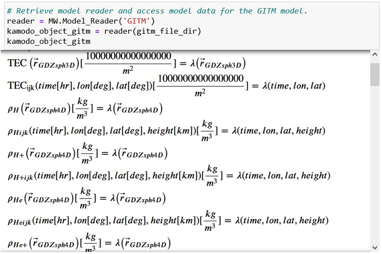
An example of a model reader interface in Kamodo. After an import statement, the user retrieves the model reader for the desired model with the first command, and then functionalizes the data with the second command of the same block. The only user-supplied information needed is which model is desired and the location of the data. The output shows the functionalized data for the variables found in the files indicated. Once the data is functionalized, all of the capabilities of Kamodo are available through simple commands. See Pembroke et al., 2022 and Ringuette et al., 2022a for more information.
Eleven types of simulation outputs are currently represented in this network, with numerous additions in process. The simulation outputs in the ITM domain include the CTIPe (Coupled Thermosphere Ionosphere Plasmasphere Electrodynamics model, Codrescu et al., 2008), IRI (International Reference Ionosphere model, Bilitza 2018), GITM (Global Ionosphere Thermosphere Model, Ridley et al., 2006), SWMF (Space Weather Modeling Framework, Toth et al., 2007, ionosphere electrodynamics portion only), TIE-GCM (Thermosphere Ionosphere Electrodynamics General Circulation Model, Qian et al., 2013), SuperDARN (Super Dual Auroral Radar Network, both the default and equal-area grids, Thomas and Shepherd, 2018), WACCM-X (Whole Atmosphere Community Climate Model with thermosphere and ionosphere extension, Liu et al., 2018), DTM (Drag Temperature Model, Bruinsma, 2015), WAM-IPE (the coupled Whole Atmosphere Model and Ionosphere Plasmasphere Electrodynamics model, Maruyama et al., 2016; Fang et al., 2022), and AMGeO (Assimilative Mapping of Geospace Observations, AMGeO Collaboration 2019) models. The eleventh simulation output is from the OpenGGCM model (Open Geospace General Circulation Model, Raeder et al., 2001, global magnetosphere outputs only). Several simulation outputs are in the process of being added: ADELPHI (AMPERE-Derive ELectrodynamic Properties of the High-latitude Ionosphere model, Robinson et al., 2021), SWMF (global magnetosphere portion), CIMI (Comprehensive Inner-Magnetosphere Ionosphere model, Fok et al., 2014), MARBLE (Bard and Dorelli, 2021, development via collaboration), and GAMERA (Grid Agnostic MHD for Extended Research Applications, Zhang et al., 2019, development via collaboration). Many more simulation outputs are planned to be added in the coming months.
We have built the first model-agnostic flythrough capability in Kamodo based on this growing network of model readers. We further add compatibility with numerous satellite trajectories by linking to repositories providing them (e.g. SSCWeb), and include coordinate conversions for a wide array of coordinate systems. The code used to provide the flythrough capability is open source and available at the official NASA Kamodo repository6. The CCMC collaborates with Ensemble Consultancy to maintain the core capabilities of Kamodo, which the described capabilities depend on (also available on GitHub7).
The remainder of this paper describes the features included in the flythrough capability, then demonstrates a few science cases it can be used for. Section 2 provides a description of the flythrough capability, including the various functions and features. This is followed by a few sample science applications in section 3, such as a model-data comparison and an ensemble modeling example. Also included in the section is an example workflow demonstrating interoperability of Kamodo with pysat, the last core PyHC (Python in Heliophysics Community8) Python package lacking such an example. Some concluding remarks and an outline of our future plans are given in section 4. Throughout the text, this paper will use italics when referring to a function or variable.
2 Kamodo’s flythrough description
Kamodo’s in-situ flythrough capability is built upon a network of model-agnostic model interfaces. These scripts provide direct access to the chosen simulation outputs with simplistic syntax that remains the same regardless of the simulation data chosen (see Figure 1 for an example). In addition to the features already described, the model readers perform linear interpolation in all time+spatial dimensions between data files and align each simulation output with a coordinate system defined by either SpacePy or AstroPy (SpacePy: Morley et al., 2011, AstroPy: AstroPy Collaboration et al., 2013 and AstroPy Collaboration et al., 2018). These uniform features allowed for a straightforward software design in the flythrough scripts.
The base function that is used for all variations of Kamodo’s flythrough capability is ModelFlythrough. This function takes the trajectory as four one-dimensional arrays of time and spatial positions and ‘flies’ the trajectory in the given coordinate system through the chosen model data in a sequence of five steps. The required inputs to the function include the trajectory arrays, coordinate system information, the chosen model and variable names, and the directory containing the model data. After some initial checks, the ModelFlythrough function (1) retrieves the model reader for the chosen model without executing the model reader script. The function then (2) compares the time values in the trajectory with the time ranges associated with the set of files in the given directory, and discards all times and their associated positions not covered by the chosen model data. The given positions are then (3) converted to the coordinate system for the given model. Next, (4) the retrieved model reader uses Kamodo to functionalize the chosen variable data for each of the model output files associated with a trajectory position, and the value of each requested variable is calculated via interpolation at the given trajectory positions. The calculated values are then (5) returned in a Python dictionary with the trajectory times and positions in the original coordinate system. Users also have the option of saving the trajectory and the corresponding variable calculations in one of three output file formats, which are all compatible with various complementary routines included in the flythrough software, such as those used in the examples in section 3. Additional output format options are planned for enhanced interoperability with other CCMC services, including CAMEL (Rastaetter et al., 2019).
The logic contained in the ModelFlythrough function is model-agnostic both in syntax and in software design as a result of the model-agnostic syntax of the model reader library. However, the various model outputs are based on quite different coordinate systems, some specific to the model, which presented a challenge. Additionally, users desired more flexibility on the trajectory input options and in the automatically-produced publication-quality visualization capabilities, so we built a small library of functions to accommodate those requests. Our current solutions to these challenges are described in the next three subsections.
2.1 Coordinate systems
Satellite trajectories are often not available in the same coordinate system as the simulation outputs. Similarly, simulation outputs are often in varying coordinate systems, making comparisons across different models difficult. For example, the AMGeO empirical model produces output in the solar magnetic coordinate system at a constant altitude, while the TIE-GCM physics-based model output instead uses geodetic coordinates with pressure level as the vertical coordinate. Directly comparing data from the two models without converting the coordinates is difficult at best due to the different rotating frames and different vertical scales of the two coordinate systems. (Note that the corresponding altitude for a given pressure level changes with location and time.) Kamodo’s flythrough simplifies this complex problem by incorporating the coordinate systems defined in AstroPy and SpacePy and the coordinate conversion functions in those packages. Model-specific coordinate conversions are handled individually within a standard framework.
Standard coordinate conversions are implemented by calling the ConvertCoord function automatically during step 3 from the utils.py script in the kamodo_ccmc/flythrough directory on GitHub. This function is a simple wrapper for the coordinate conversion capabilities in the AstroPy and SpacePy packages, and is written both for automatic execution by the flythrough functions and for direct user interaction. The input variables include the one dimensional arrays for the time and spatial coordinate values, and a few strings for the user to indicate the input and output coordinate systems. ConvertCoord determines which software package the input and output coordinate systems belong to, creates the appropriate coordinate object using the input data, performs the coordinate conversion, and returns the new coordinate values in one dimensional arrays (see the Trajectory_Coords_Plots notebook for more details9 and Figure 2 below for a concept map). However, the function can only be used when both the input and output coordinate systems are defined in one of the two packages mentioned.
FIGURE 2
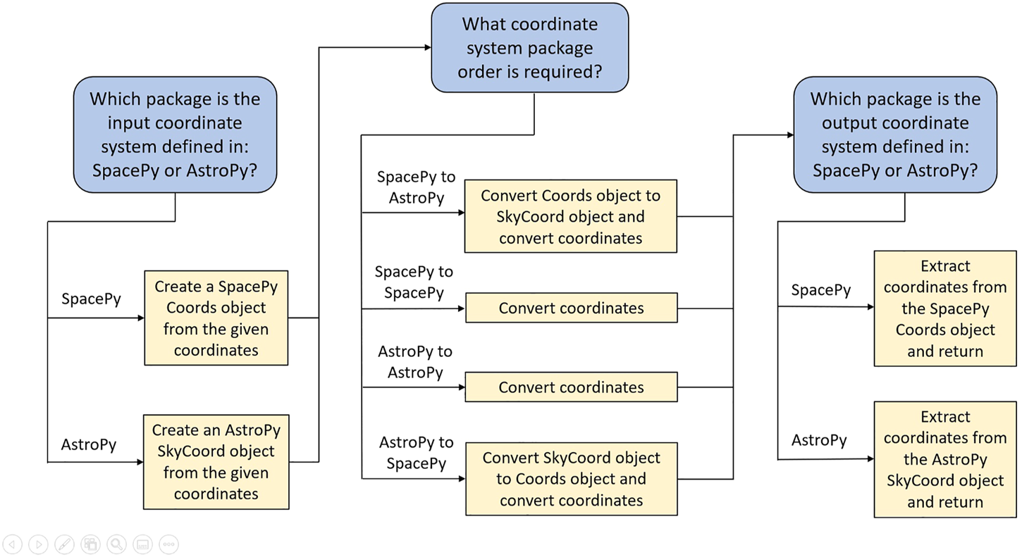
Concept map for the ConvertCoords function. Blue boxes indicate conditional arguments, yellow boxes show tasks executed depending upon the evaluation result of the preceding conditional argument. Error catching logic is not included in the figure for simplicity. The inputs to the argument include one dimensional arrays of the time and spatial coordinates (4 1D arrays), and four strings indicating the input and output coordinate systems and whether each is Cartesian or spherical. The values returned are one dimensional arrays of the spatial coordinates (3 1D arrays) and a list of strings containing the units of the output coordinates. Model-specific coordinates are handled external to this function.
Some simulation outputs are given in a coordinate system specific to the model and not defined in either the AstroPy or SpacePy software packages. In those cases, we rely on custom coordinate conversion functions in the model readers to link between a coordinate system defined in either package and the coordinate system defined in the model. Current examples of this work can be found in the CTIPe and TIE-GCM model readers for conversions between pressure level and altitude. This approach uses Kamodo’s function composition capabilities, and will soon be applied to models with more complex coordinate systems, such as those based on pitch angle and energy (Ringuette et al., 2022a). By linking the model-specific coordinate system to a coordinate system defined in one of the linked packages, the flythrough functionality will then be able to convert to any desired coordinate system. Collaborations with model developers on this challenge have begun for a few models.
2.2 Input trajectories
During the initial development, we identified five possible types of desired input methods for satellite trajectories: one from satellite ephemerides obtained from SSCWeb, one from a file of two-line elements (TLEs), one from a file of previously obtained satellite positions, one from a variable defined in the user’s Python session memory, and one from a sample trajectory generator. To avoid duplicated code across the five possibilities, we chose the session memory example as the simplest example and designed the base functionality accordingly (the ModelFlythrough function described above). The remaining flythrough functions call the various specific trajectory functions and then call the ModelFlythrough function to perform the flythrough.
The five flythrough functions are the RealFlight, TLEFlight, FakeFlight, MyFlight, and ModelFlythrough functions (see Table 1). As mentioned above, the ModelFlythrough function takes the given trajectory, provided as four one-dimensional arrays, and flies it through the chosen simulation output. The RealFlight function calls the SatelliteTrajectory function to retrieve a real satellite trajectory in the form of four one-dimensional arrays from the SSCWeb10 through an existing HAPI interface for this resource (Weigel et al., 2021). The function then calls the ModelFlythrough function to fly that trajectory through the data. An alternative option is provided with the TLEFlight function, which calls the TLETrajectory function to convert TLEs into a trajectory of the same structure as above using the SGP4 propagator (Simplified General Perturbations11: Vallado and Crawford 2008). The four one-dimensional arrays containing the trajectory information are then fed to the ModelFlythrough function as before. Similarly, the MyFlight function allows the user to provide the trajectory through a simply structured file either in comma-separated, tab-separated, or netCDF4 format options, and then calls ModelFlythrough. This function was specifically designed to easily fly a previously saved trajectory through a different set of model data to simplify comparisons across multiple models and model outputs. This capability has proved especially useful for users desiring to use a real satellite trajectory previously used but finding themselves without internet access.
TABLE 1
| Function name | Minimum syntax required | Trajectory source |
|---|---|---|
| ModelFlythrough | ModelFlythrough (model, file_dir, variable_list, sat_time, c1, c2, c3, coord_sys) | Session memory |
| RealFlight | RealFlight (dataset, start, stop, model, file_dir, variable_list) | SSCWeb via SatelliteTrajectory |
| TLEFlight | TLEFlight (tle_file, start, stop, time_cadence, model, file_dir, variable_list) | Text file containing TLEs via TLETrajectory |
| FakeFlight | FakeFlight (start_time, stop_time, model, file_dir, variable_list) | SampleTrajectory |
| MyFlight | MyFlight (traj_file, model, file_dir, variable_list) | File previously produced by a flythrough function |
Flythrough Functions. The function names are followed by the minimum syntax required for each of the four flythrough functions. The source of each of the trajectories is indicated in the last column. SatelliteTrajectory, TLETrajectory, and SampleTrajectory are functions available through the flythrough software. See text for a basic description of each, and the example notebooks and documentation for more information8.
Finally, the FakeFlight function calls the SampleTrajectory function, which constructs a sample satellite trajectory based on a variety of input parameters, and then flies that trajectory through the simulation output using the ModelFlythrough function. The simplest call to the SampleTrajectory function only requires start and end times in UTC to create a synthetic trajectory in geodetic spherical coordinates similar in nature to a low earth orbit (see Figure 3). Various default values can be adjusted in the function call to change the longitudinal precession rate per orbit, the maximum and minimum latitudes, the maximum and minimum initial heights, the decay rate of the height, and the time cadence of the returned positions. The trajectory produced by the SampleTrajectory function is not meant to fully simulate any actual satellite orbit, but to simply give users a reasonable starting point if no actual trajectory is decided upon yet. The three trajectory functions, SatelliteTrajectory, TLETrajectory, and SampleTrajectory, may also be called independent of the other functions for additional uses, such as retrieving and modifying a real satellite trajectory before flying it through a set of model data, or visualizing a trajectory created from TLEs. Because these five flythrough functions are based on a network of readers with model-agnostic syntax, the flythrough function syntaxes are also model-agnostic.
FIGURE 3
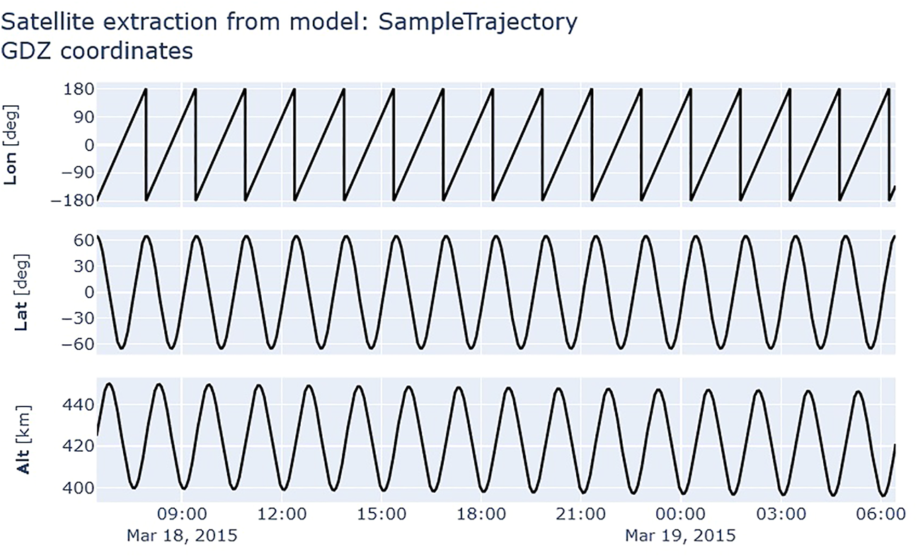
The default trajectory produced by the SampleTrajectory function. Together, the plots show the position of the imaginary satellite in geodetic spherical coordinates (longitude, latitude, and altitude) for a 24-h period. Note the longitude begins at -180 but ends slightly above that value due to the precession in longitude, which can be chosen by the user. The default latitude range is centered on the equator as shown, but any continuous range can be chosen. By default, the altitude varies in each orbit and degrades slowly over time. The rate of degradation can also be adjusted via an input parameter. See documentation for more details9.
An example of Kamodo’s RealFlight function is presented in Figure 4. The first block shows the two required import statements followed by the definition of various input values. The input values related to the satellite should be determined using the SSCWeb website9. The parameters related to the simulation output data, such as the time values in UTC timestamps (start_utcts and end_utcts, the number of seconds since 1 January 1970 at midnight UTC) and the variable names, can be obtained using the various functions demonstrated in the SF_IntroFunctions notebook8. The second block shows the syntax of the RealFlight function, which is notably identical regardless of the model chosen. The final block shows a simple method to functionalize the object returned by the function call. Note that the TIE-GCM model outputs use pressure level as the vertical coordinate, but no additional commands or parameters are needed as the conversions between pressure level and altitude (or radius) are handled internally and automatically.
FIGURE 4
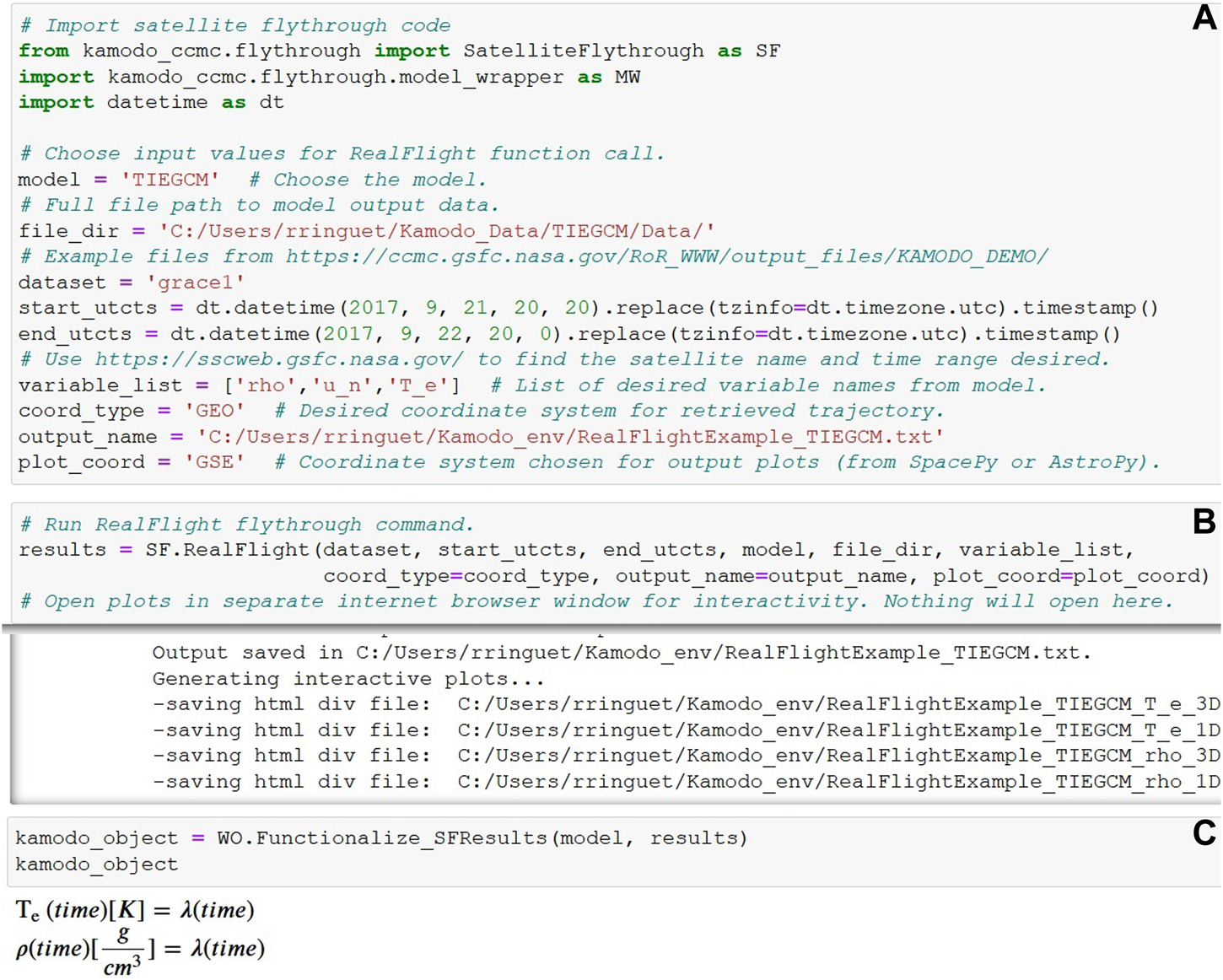
Example notebook demonstrating the model-agnostic syntax of the RealFlight flythrough function. The first block (A) shows the two required import statements and chosen variable values. The datetime package is imported to deal with the generation of the UTC timestamps. The second block (B) presents the model-agnostic syntax of the function call, and the last block (C) shows a simple way to functionalize the Python object returned by the flythrough function.
Regardless of the flythrough function chosen, the object returned by each function call is identical in structure. Consequently, the Functionalize_SFResults function can be used to functionalize any of these objects. Once the returned object is functionalized, all of the previously described core capabilities of Kamodo are available to the user, including simplistic access to interactive plotting (see the bottom section of Figure 7 below).
2.3 Custom visualizations
If the user defines the name of the output file in any of the flythrough function calls, then the resulting data is written to the named file and two custom visualizations are automatically generated for each variable (see Figures 5, 6 below). Both visualizations are designed using Plotly (Plotly Technologies Inc, 2015), and are produced by calling the SatPlot4D function with different parameters (see the SF_Traj_Coords_Plots notebook for details8).
FIGURE 5
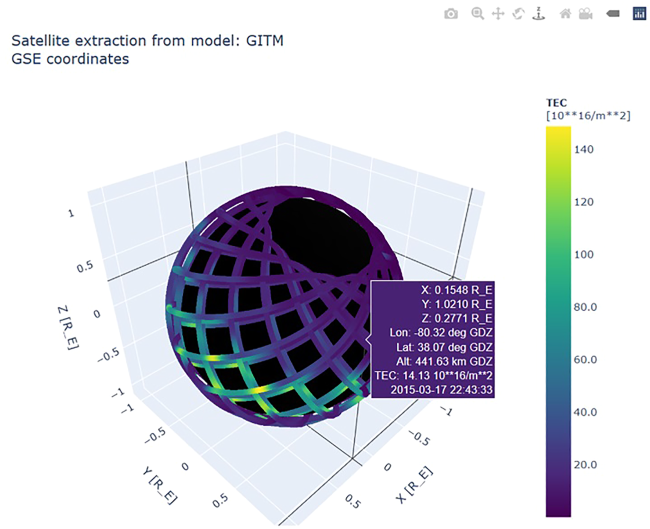
An example of a fully interactive 3D plot. In this case, the total electron content (TEC) is plotted for the entirety of a given satellite trajectory. TEC values are indicated by the colorbar at right, and the model source and coordinate system are printed in the top left corner. The purple box contains the coordinate information in GSE coordinates, both in Cartesian and spherical, the TEC value, also indicated by the color of the box, and the date and time in UTC for the data point hovered over by the mouse. The symbols on the top right are the typical buttons provided by Plotly. The plot is saved as a fully interactive html file. An example is included on the NASA Kamodo repository5.
FIGURE 6

An example of a fully interactive 1D plot. As in Figure 5, the total electron content (TEC) is plotted for the entirety of a given satellite trajectory at top (A), followed by the trajectory parameters in Cartesian coordinates in the remaining three plots (B–D). The model source and coordinate system are printed in the top left corner. Hovering over a value in any of the plots gives a box containing the value and the date and time in UTC. The symbols on the top right are the typical buttons provided by Plotly. The plot is saved as a fully interactive html file. An example is included on the NASA Kamodo repository5.
Figure 5 shows the full interactive spatial representation of the entire chosen trajectory in GSE coordinates. The colors indicate the total electron content (TEC) at the given location and time, as indicated by the colorbar at right. Users can pan, zoom, and hover over the image to inspect more closely. All interactivity is saved to an html file. Figure 6 shows the same information plotted as four time series. Zooming into one of the four plot sections results in the same zooming for the other three plots. Similar versions of these plots are saved on the NASA Kamodo repository8. Several options are available, especially for plots similar to Figure 5, and are explained in the referenced notebook. For additional visualization capabilities, see Ringuette et al., 2022a.
3 Example science workflows
Kamodo’s model-agnostic flythrough capability reduces data-model, model-model comparisons, and even ensemble modeling analysis to a few lines of code, regardless of the model or trajectory desired. Examples of these applications are given in the following subsections, followed by an example of interoperability of Kamodo with pysat. Links to examples of interoperability of Kamodo with the remaining PyHC core packages are also given in this section. In addition to being used in the example workflows, the flythrough capability is being used from the command line to incorporate physics-based models into GEODYN II, an orbit propagator written in FORTRAN (Luthcke et al., 2006; Garcia-Sage et al., 2021).
3.1 Model-data comparison workflow
Simplistic data-model comparisons using in-situ data are now possible with a few lines of code for an expanding range of models and a wide range of trajectories. Combining the RealFlight function demonstrated in Figure 4 with the CDAWeb12 interface in Kamodo results in the simple workflow displayed in Figure 7. The top block in the figure uses the syntax taken from Figure 4 to fly the chosen satellite through the model data produced by the TIE-GCM model. The time range of the model data was chosen to cover the time range of the desired observational data. We note that any of the flythrough functions can be interchanged in place of the RealFlight function shown in the example without changing the syntax of the remaining blocks due to the identical data structures returned.
FIGURE 7
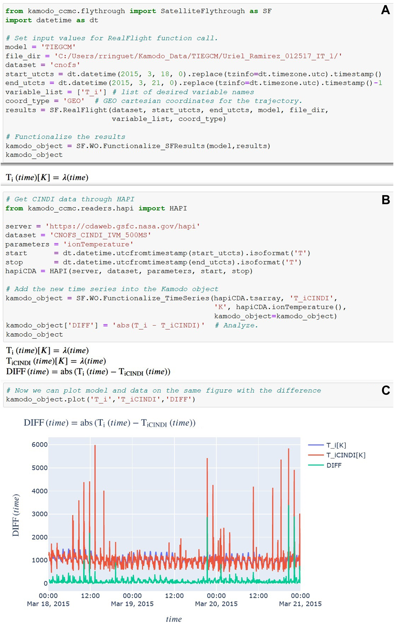
Example of model-data comparison. The first block (A) uses Kamodo’s RealFlight function to fly the chosen satellite trajectory through the chosen simulation output. The second block (B) retrieves the ion temperature data from the same satellite and adds it to the previously created kamodo_object variable. The difference between the two datasets is easily calculated via function composition. A fully interactive plot showing the three variables is easily created in the third block (C).
In this case, the observational dataset is the ion temperature observed by the Coupled Ion-Neutral Dynamics Investigations (CINDI) mission (Coley et al., 2010). Retrieval of the data is demonstrated in the second block. The parameter values shown in that block can be determined through the CDAWeb website. Once the data is retrieved, it can be easily functionalized using the Functionalize_TimeSeries function as shown in the same block. Note that this function can only be used to functionalize one dimensional time series data. Other methods are available to functionalize higher dimensionality data (see Kamodo documentation4). Once both the simulated and observed data are functionalized, all of the core capabilities available through Kamodo are easily accessible, including the fully interactive plotting shown in the bottom block. We note the two datasets are plotted using their original time resolutions - every minute for the TIE-GCM simulation output and every second for the CINDI data. The ‘DIFF’ dataset generated by function composition in the second block is calculated and plotted using the finer time resolution of the CINDI dataset. Additional observational and simulated datasets can be added and functionalized using the same syntax to extend the comparison.
3.2 Ensemble modeling example workflow
Expanding the model-data comparison to include multiple models leads to another science use case called ensemble modeling. (We use the term ‘ensemble modeling’ in the same sense as in hurricane track prediction, which means to predict a given variable based on the distribution of predictions given by various models.) In this use case, the desired flythrough is called once for each simulation output per desired trajectory. Once the outputs are functionalized, function composition can be used to combine the results in a weighted average, even if the weights depend on another parameter.
Figure 8 below demonstrates a simple example of such a workflow. Two simulation outputs from different models were prepared for the same time range. For simplicity, the example uses the same trajectory function as in Figure 4 to fly the C/NOFS trajectory through both simulation outputs (blocks 1 and 2). The next block shows how to pull the results from each RealFlight function call into the same Kamodo object. This block also shows how to use the function composition capability in Kamodo-core to combine the results from each into a custom average calculation. Plotting any or all of the functions is similarly simplistic as in Figure 7, but is not shown for brevity. This workflow can be easily expanded to include additional simulation outputs, more complex functions, unit conversions, and other useful features.
FIGURE 8
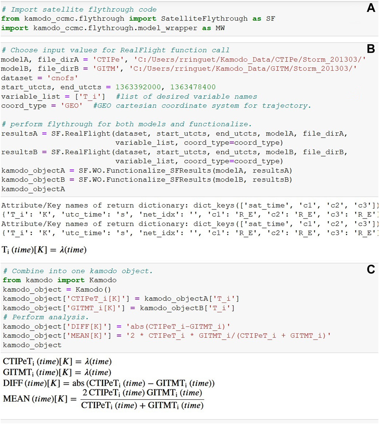
Example of ensemble modeling workflow. The first two blocks (A and B) use Kamodo’s RealFlight function to fly the chosen satellite trajectory through two simulation outputs. In the third block (C), the functions are collected into a single Kamodo object for further computation via function composition.
3.3 Interoperable workflows
Kamodo is now one of the core packages in the PyHC group and is also interoperable with all of the other core packages. An example workflow of analyzing MMS data (Polson et al., 202213) demonstrates the interoperability of Kamodo with several other Python packages, including SpacePy, PlasmaPy, and pySPEDAS14 (PlasmaPy Community 2022). Another workflow shown at the 2022 PyHC Summer School demonstrated using SunPy and Kamodo together15. Finally, an interface exists between the pysat and kamodo packages16, but no workflow using the two packages is known to exist.
In this section, we feature a workflow combining pysat and Kamodo to compare simulated and observed data (Figure 9). The workflow presented in Figure 9 is identical to the workflow presented in section 3.1, but instead uses pysat to retrieve the desired data. We adapted code from the pysat example notebooks given at the 2022 PyHC Summer School to implement pysat in this manner. One advantage to this choice is to use the data filtering in pysat to clean the observed data before comparing it with the simulated data, which results in a better comparison to the simulated data.
FIGURE 9
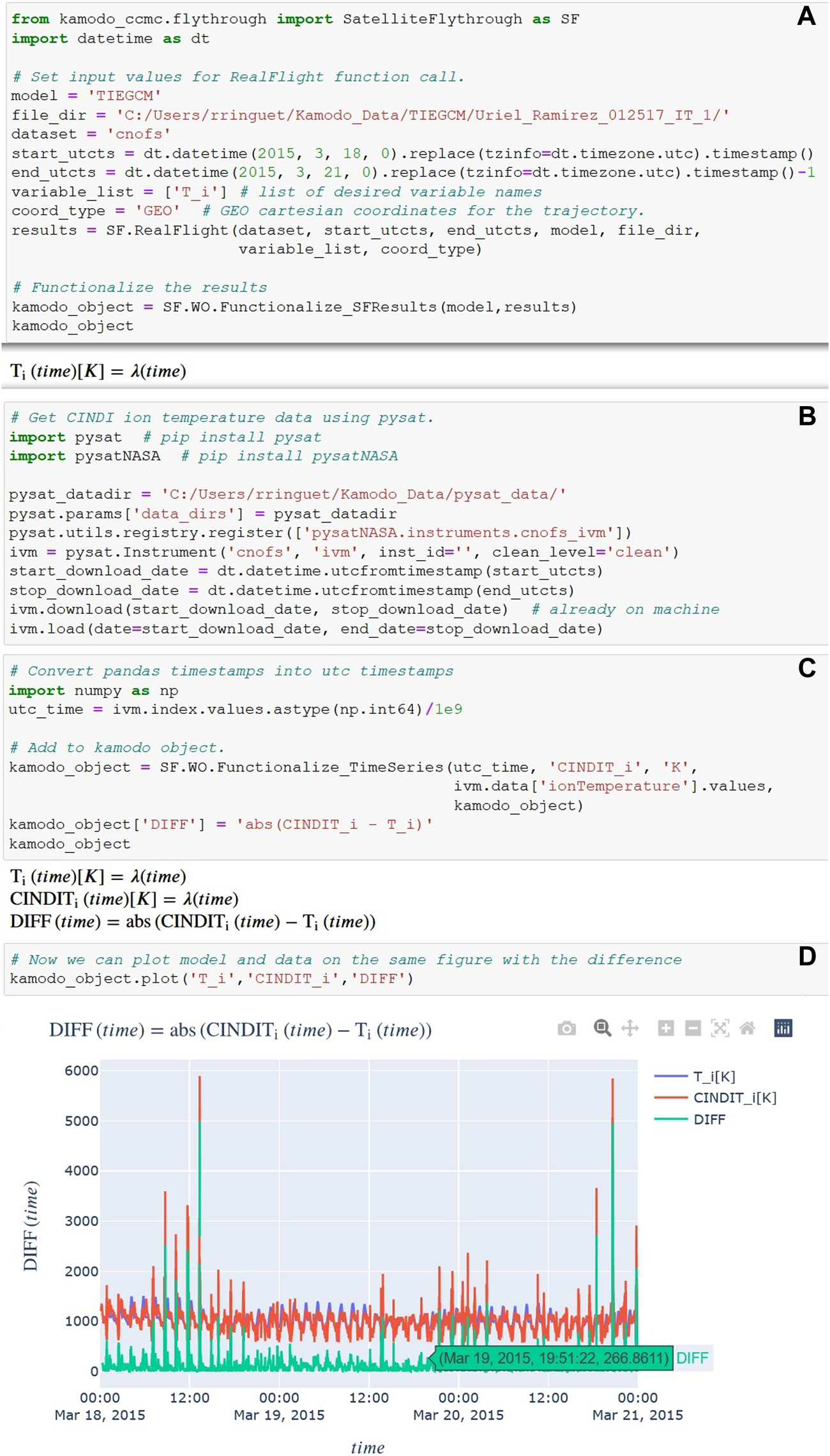
Example of model-data comparison using pysat and Kamodo. The first block (A) is identical to the first block of Figure 7. The second block (B) proceeds to use pysat to retrieve the same data as in Figure 7, but applies the data cleaning routines for the data implemented in pysat. The next block (C) converts the times to UTC timestamps, functionalizes the data, and adds the functionalized data to the existing Kamodo object. The output of the final block (D) is similar to that of Figure 7, but now contains the cleaned observational data instead of the raw data.
Comparing the final plots at the bottom of Figures 7, 9 shows the differences between the two analysis methods, especially the reduction and removal of several spikes in the data in Figure 9 as compared to Figure 7 (orange in both plots). As noted in the model-data comparison presented in section 3.1, the simulated data is plotted using its original time cadence of every minute, and the CINDI data and ‘DIFF’ function are plotted every second, with identical timestamps as in Figure 7. The exception to this 17results from the data removed by the cleaning process. Figure 10 shows the data gaps in the cleaned CINDI data in a zoomed-in section of the graph centered on the spike just before 1600 UTC on 18 March 2015 as compared to the original data retrieved via Kamodo’s CDAWeb HAPI interface. These data gaps are propagated to the DIFF function automatically as part of the function composition.
FIGURE 10
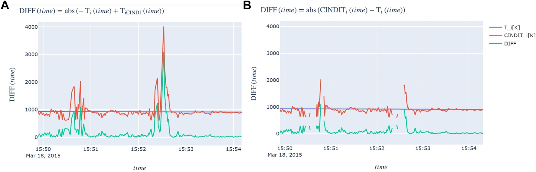
Comparison of the model-data comparison workflow results using only Kamodo (left, (A) and pysat+Kamodo (right, (B). The data shown in both plots are approximately 4 min sections of the plots shown in Figure 7 and Figure 9 (less than 1/20 of an orbit). The axes in each plot are nearly identical, with the TIE-GCM dataset shown in blue (nearly horizontal lines near 1000 K), the CINDI dataset represented in orange, and the DIFF calculated function in green. The time cadences and values in each plot are identical, except for the data gaps in the right plot. These gaps result from the data cleaning routines developed for the CINDI data in pysat, and are automatically propagated to the DIFF function in the function composition performed using Kamodo.
The simulated data and the chosen observational dataset in this workflow can both be changed to the user’s specific goal, along with the dates and the analysis function. In the future, we are eager to use pysat’s developing interface to orbit propagators as input to Kamodo’s flythrough functions, and to use Kamodo to incorporate physics-based models into those orbit propagators.
4 Summary
Kamodo’s satellite flythrough capability decreases the utilization barrier for heliophysics model outputs by providing a model-agnostic utility for the entire community. As the library of models implemented in Kamodo expands, so will the capability of the flythrough tools. Our first focus has been to add a variety of ionosphere-thermosphere-mesosphere simulation outputs to Kamodo in support of the upcoming Geospace Dynamics Constellation mission. We are continuing to add more simulation outputs to Kamodo in this domain, and are now expanding our efforts into the geospace domain. Expanding to include geospace model outputs requires a new approach to coordinate conversions due to the often model-specific coordinate systems involved (see Ringuette et al., 2022a). However, this is easily incorporated into the current software architecture by using the function composition capability inherent in Kamodo. Further expansion into heliosphere and solar physics model outputs is also planned. We intend for Kamodo to become the new user interface for interacting with all model outputs on the CCMC website, including the Instant Run, Runs-on-Request, and real-time model output visualization interfaces. Accomplishing this goal will require increasing the capability well beyond what is currently offered. Kamodo’s continuing development as open-source software will also deliver the same powerful solution for users on their own computers and on the cloud.
Additional capabilities based on the flythrough are also in development. For example, we have developed a satellite constellation mission planning tool in support of the Geospace Dynamics Constellation mission (Pfaff, 2016) that is now available on GitHub as part of the Kamodo CCMC software package for user testing. To increase accessibility of model outputs, we are beginning work on adding HAPI as a layer on top of the RealFlight and TLEFlight flythrough functions and on top of the model reader interfaces. This will enable the community to more easily access and download model outputs by only serving the desired portions of the data instead of serving the often prohibitively large files. We are also working to improve CCMC’s Kamodo documentation, especially including sample workflows similar to the ones included in this work. Simple additions planned in the short-term include code refactoring to generalize the treatment of model-specific coordinate conversions, and additional sample workflows. Long term development goals include a line of sight calculation tool and a simulated imagery tool to expand beyond in-situ applications, cloud capabilities, nowcasting with continuous runs, satellite drag modeling18, and reduced code and code-free interfaces to model outputs (see Figure 6, Figure 7 of Ringuette et al., 2022b).
Building these capabilities on top of Kamodo provides a powerful foundation for a large range of exciting capabilities, especially for the complex case of simulation outputs. Since Kamodo works for any data, our work can be easily extended into other areas, even outside of the science and research communities entirely. Applying Kamodo to heliophysics simulated and observed data is beginning to lower the utilization barrier for the entire community. Collaborators are welcome!
Statements
Data availability statement
Publicly available datasets were analyzed in this study. This data can be found here: The simulated datasets analyzed for this study can be found in the Kamodo Demo directory at CCMC (https://ccmc.gsfc.nasa.gov/RoR_WWW/output_files/KAMODO_DEMO/). Additional model outputs can be accessed through the CCMC (https://ccmc.gsfc.nasa.gov/). The observational dataset from the CINDI instrument analyzed in this work is available through NASA SPDF’s CDAWeb HAPI service (https://cdaweb.gsfc.nasa.gov/index.html).
Author contributions
RR wrote the text of the article, developed and tested the flythrough functions described, and generated figures. DD developed the visualization codes and coordinate conversion codes to support the flythrough functions. LR directed the development of the flythrough functions. DD and LR assisted in testing of the software and feedback on its functionality during development. AP and OG supported the required functionality by developing and maintaining the Kamodo-Core software package that the CCMC-Kamodo package depends on. KG-S assisted in the development of the TLETrajectory function. LR, DD, OG, and KG-S also provided feedback on the article content.
Funding
RR’s work was funded by the CCMC through ADNET Systems, Inc. DD‘s work was funded by the CCMC through the Catholic University of America. LR‘s and KG-S‘s work was funded directly by the CCMC. AP and OG’s work were funded via a NASA SBIR Phase 2: Space Weather R2O/O2R Technology Development grant titled “Kamodo Containerized Space Weather Models” (Contract #80NSSC20C0290) awarded to Ensemble Government Services, LLC. The funder was not involved in the study design, collection, analysis, interpretation of data, the writing of this article or the decision to submit it for publication.
Acknowledgments
RR acknowledges Russell Stoneback for helpful comments on the pysat-Kamodo notebooks. This work uses simulation results from the Community Coordinated Modeling Center at Goddard Space Flight Center. The CCMC is a multi-agency partnership between NASA, AFMC, AFOSR, AFRL, AFWA, NOAA, NSF, and ONR. We also acknowledge the use of CINDI data from the C/NOFS mission, which was provided by the CINDI team at the University of Texas at Dallas, made available through NASA SPDF’s CDAWeb HAPI service. The CINDI team was supported by NASA grant NAS5-01068. See https://hpde.io/NASA/NumericalData/CNOFS/CINDI/IVM/PT0.5S.html.
Conflict of interest
Author RR was employed by ADNET Systems Inc., a contractor for NASA GSFC. Authors AP and OG were employed by Ensemble Government Services.
The remaining authors declare that the research was conducted in the absence of any commercial or financial relationships that could be construed as a potential conflict of interest.
Publisher’s note
All claims expressed in this article are solely those of the authors and do not necessarily represent those of their affiliated organizations, or those of the publisher, the editors and the reviewers. Any product that may be evaluated in this article, or claim that may be made by its manufacturer, is not guaranteed or endorsed by the publisher.
Footnotes
1.^https://sscweb.gsfc.nasa.gov/.
2.^See https://ccmc.gsfc.nasa.gov/results/index.php, search for existing simulation runs, and use one of the timeseries visualization links (e.g., “Timeseries in Magnetosphere”) in each run’s page, see https://ccmc.gsfc.nasa.gov/results/viewrun.php?domain=GM&runnumber=Junying_Yang_042021_1 for a specific example and click on one of the links at the bottom of the page/
3.^See https://ccmc.gsfc.nasa.gov/ungrouped/GM_IM/GM_analysis.php, and https://ccmc.gsfc.nasa.gov/ungrouped/GM_IM/GM_analysis.php?Pid=21127&Pt=BO&Ps=Cluster-1 for a specific example.
4.^https://pysat.readthedocs.io/en/latest/instruments/pysatModels.html.
5.^https://ensemblegovservices.github.io/kamodo-core/.
6.^https://github.com/nasa/Kamodo.
7.^https://github.com/EnsembleGovServices/kamodo-core.
9.^https://github.com/nasa/Kamodo/tree/master/docs/notebooks.
10.^https://sscweb.gsfc.nasa.gov/.
11.^https://pypi.org/project/sgp4/,https://help.agi.com/stk/index.htm#stk/vehSat_orbitProp_msgp4.htm.
12.^https://cdaweb.gsfc.nasa.gov/index.html.
13.^https://deepnote.com/workspace/shawn-polson-c095a0fb-f02d-416d-9c94-c4a9c4e8e54d/project/PyHC-Paper-101b9646-3fd0-4978-a48e-a4f3e708a0ac/%2FMaking_an_Executable_Paper_with_the_Python_in_Heliophysics_Community_to_Foster_ Open_Science_and_Improve_Reproducibility_ipynb.
14.^https://pyspedas.readthedocs.io/en/latest/.
15.^https://github.com/heliophysicsPy/summer-school/tree/main/kamodo-tutorial.
16.^https://pypi.org/project/pysat-kamodo/.
17.^https://github.com/heliophysicsPy/summer-school.
18.^See http://alpha.drag.ensemblespacelabs.com:1234/, and https://www.youtube.com/watch?v=vpJgtAMCVvc&ab_channel=Ensemble for a tutorial video.
References
1
AMGeO Collaboration (2019). A collaborative data science platform for the geospace community: Assimilative mapping of geospace observations (AMGeO) v1.0.0. Zenodo. 10.5281/zenodo.3564914
2
AstroPy Collaboration, TollerudE. J.GreenfieldP.DroettboomM.BrayE.AldcroftT.DavisM.et al (2013). Astropy: A community Python package for astronomy. Astron. Astrophys.558, A33. 10.1051/0004-6361/201322068
3
AstroPy Collaboration, SipoczB. M.GuntherH. M.LimP. L.CrawfordS. M.ConseilS.ShupeD. L.et al (2018). The astropy project: Building an open-science project and status of the v2.0 core package. Astron. J.156 (3), 123. 10.3847/1538-3881/aabc4f
4
BardC.DorellliJ. C. (2021). Magnetotail reconnection asymmetries in an ion-scale, Earth-like magnetosphere. Ann. Geophys.39, 991–1003. 10.5194/angeo-39-991-2021
5
BilitzaD. (2018). IRI the international standard for the ionosphere. Adv. Radio Sci.16, 1–11. 10.5194/ars-16-1-2018
6
BruinsmaS. (2015). The DTM-2013 thermosphere model. J. Space Weather Space Clim.5, A1. 10.1051/swsc/2015001
7
CodrescuM. V.Fuller-RowellT. J.MunteanuV.MinterC. F.MillwardG. H. (2008). Validation of the coupled thermosphere ionosphere plasmasphere electrodynamics model: CTIPe-mass spectrometer incoherent scatter temperature comparison. Space6, S09005. 10.1029/2007SW000364
8
ColeyW. R.HeelisR. A.HairstonM. R.EarleG. D.PerdueM. D.PowerR. A.et al (2010). Ion temperature and density relationships measured by CINDI from the C/NOFS spacecraft during solar minimum. J. Geophys. Res.115, A02313. 10.1029/2009JA014665
9
FangT.-W.KubarykA.GoldsteinD.LiZ.Fuller-RowellT.MillwardG.et al (2022). Space weather environment during the spaceX starlink satellite loss in february 2022. Space Weather20, e2022SW003193. 10.1029/2022SW003193
10
FokM.-C.BuzulukovaN. Y.ChenS.-H.GlocerA.NagaiT.ValekP.et al (2014). The comprehensive inner magnetosphere-ionosphere model. J. Geophys. Res. Space Physics119, 7522–7540. 10.1002/2014JA020239
11
Garcia-SageK.WaldronZ.RowlandsD.LemoineF.SuttonE.ThayerJ.et al (2021). Expanding and testing orbit propagation capabilities using CCMC-hosted models. Washington, DC: American Geophysical Union. Presented at the AGU Fall Meeting 2021, 13-17 December 2021, id. SA31B-04. Available at: https://ui.adsabs.harvard.edu/abs/2021AGUFMSA31B.04G/abstract.
12
LiuH.-L.BardeenC. G.FosterB. T.LauritzenP.LiuJ.LuG.et al (2018). Development and validation of the whole Atmosphere community climate model with thermosphere and ionosphere extension (WACCM-X 2.0). J. Adv. Model. Earth Syst.10, 381–402. 10.1002/2017MS001232
13
LuthckeS. B.RowlandsD. D.LemoineF. G.KloskoS. M.ChinnD.McCarthyJ. J. (2006). Monthly spherical harmonic gravity field solutions determined from GRACE inter-satellite range-rate data alone. Geophys. Res. Lett.33, L02402. 10.1029/2005GL024846
14
MaruyamaN.SunY.-Y.RichardsP. G.MiddlecoffJ.FangT.-W.Fuller-RowellT. J.et al (2016). A new source of the midlatitude ionospheric peak density structure revealed by a new Ionosphere-Plasmasphere model. Geophys. Res. Lett.43. 10.1002/2015GL067312
15
MorleyS. K.WellingD. T.KollerJ.LarsenB. A.HendersonM. G.NiehofJ.et al (2011). “SpacePy - a python-based library of tools for the Space sciences,” in Proceedings of the 9th Python in Science Conference, Austin, TX, July 11–17, 2010, p. 67–72. Editors vad der WaltS.MillmanJ.. 10.25080/Majora-92bf1922-00c
16
PembrokeA.De ZeeuwD.RastaetterL.RinguetteR.GerlandO.PatelD.et al (2022). Kamodo: A functional api for space weather models and data. J. Open Source Softw.7, 4053. 10.21105/joss.04053
17
PfaffR. F.Jr. (2016). An overview of the scientific and space weather motivation for the “Notional” geospace dynamics constellation mission. American Geophysical Union, Fall General Assembly. Available at: https://ui.adsabs.harvard.edu/abs/2016AGUFMSA23C..01P
18
PlasmaPy Community (2022). PlasmaPy, version 0.8.1. Zenodo. 10.5281/zenodo.6774350
19
Plotly Technologies Inc (2015). Collaborative data science. Montréal, QC: Plotly Technologies Inc. https://plot.ly.
20
PolsonS.RinguetteR.RastaetterL.GrimesE.NiehofJ.MurphyN. A.et al (2022). Making an executable paper with the python in heliophysics community to foster open science and improve reproducibility. Front. Astron.Under review.
21
QianL.BurnsA.EmeryB.FosterB.LuG.MauteA.et al (2013). The ncar TIE-GCM: A community model of the coupled thermosphere/ionosphere system. Geophys. Monogr. Ser.201, 73–83. 10.1029/2012GM001297
22
RaederJ.WangY. L.Fuller-RowellT. J.SingerH. J. (2001). Global simulation of space weather effects of the Bastille Day storm. Sol. Phys.204, 325. 10.1023/A:1014228230714
23
RastaetterL.WiegandC.MullinixR.MacNieceP. J. (2019). Comprehensive assessment of models and events using library tools (camel) framework: Time series comparisons. Space Weather17 (6), 845–860. 10.1029/2018SW002043
24
RidleyA.DengY.TóthG. (2006). The global ionosphere–thermosphere model. J. Atmos. Solar-Terrestrial Phys.68, 839–864. 10.1016/j.jastp.2006.01.008
25
RidleyA. J.De ZeeuwD. L.RastätterL. (2016). Rating global magnetosphere model simulations through statistical data-model comparisons. Space14, 819–834. 10.1002/2016SW001465
26
RinguetteR.EngellA.GerlandO.McGranaghanR. M.ThompsonB. (2022b). The DIARieS ecosystem – a software ecosystem to simplify discovery, implementation, analysis, reproducibility, and sharing of scientific results and environments in Heliophysics. Adv. Space Res. 10.1016/j.asr.2022.05.012
27
RinguetteR.RastätterL.De ZeeuwD. L.PembrokeA.GerlandO. (2022a). Simplifying model data access and utilization. Adv. Space Res. under review.
28
RobinsonR. M.ZanettiL.AndersonB.VinesS.GjerloevJ. (2021). Determination of auroral electrodynamic parameters from AMPERE field-aligned current measurements. Space19, e2020SW002677. 10.1029/2020SW002677
29
StonebackR.BurrellA. G.KlenzingJ.DepewM. D. (2018). PYSAT: Python satellite data analysis toolkit. JGR. Space Phys.123, 5271–5283. 10.1029/2018JA025297
30
ThomasE. G.ShepherdS. G. (2018). Statistical patterns of ionospheric convection derived from mid-latitude, high-latitude, and polar SuperDARN HF radar observations. J. Geophys. Res. Space Phys.123 (4), 3196–3216. 10.1002/2018JA025280
31
TothG.De ZeeuwD. L.GombosiT. I.ManchesterW. B.RidleyA. J.SokolovI. V.et al (2007). Sun-to-thermosphere simulation of the 28-30 october 2003 storm with the space weather modeling framework. Space5, S06003. 10.1029/2006SW000272
32
ValladoD.CrawfordP. (2008). “SGP4 orbit determination,” in AIAA/AAS Astrodynamics Specialist Conference and Exhibit, Honolulu, Hawaii, August 18–21, 2008 (Reston, VA: American Institute of Aeronautics and Astronautics). 10.2514/6.2008-6770
33
WeigelR. S.VandegriffJ.FadenJ.KingT.RobertsD. A.HarrisB.et al (2021). HAPI: An API standard for accessing heliophysics time series data. JGR. Space Phys.126, 12. 10.1029/2021JA029534
34
ZhangB.SorathiaK. A.LyonJ. G.MerkinV. G.GarretsonJ. S.WiltbergerM. (2019). Gamera: A three-dimensional finite-volume MHD solver for non-orthogonal curvilinear geometries. Astrophys. J. Suppl. Ser.244, 20. 10.3847/1538-4365/ab3a4c
Summary
Keywords
data, heliophysics, python (programming language), simulation, model-data comparisons, ensemble modeling, flythrough, data functionalization
Citation
Ringuette R, De Zeeuw D, Rastaetter L, Pembroke A, Gerland O and Garcia-Sage K (2022) Kamodo’s model-agnostic satellite flythrough: Lowering the utilization barrier for heliophysics model outputs. Front. Astron. Space Sci. 9:1005977. doi: 10.3389/fspas.2022.1005977
Received
28 July 2022
Accepted
02 November 2022
Published
05 December 2022
Volume
9 - 2022
Edited by
Angeline G. Burrell, United States Naval Research Laboratory, United States
Reviewed by
Bruce Fritz, United States Naval Research Laboratory, United States
Scott England, Virginia Tech, United States
Updates
Copyright
© 2022 Ringuette, De Zeeuw, Rastaetter, Pembroke, Gerland and Garcia-Sage.
This is an open-access article distributed under the terms of the Creative Commons Attribution License (CC BY). The use, distribution or reproduction in other forums is permitted, provided the original author(s) and the copyright owner(s) are credited and that the original publication in this journal is cited, in accordance with accepted academic practice. No use, distribution or reproduction is permitted which does not comply with these terms.
*Correspondence: Rebecca Ringuette, Rebecca.ringuette@gmail.com
†ORCID: Asher Pembroke, orcid.org/0000-0002-5718-1303; Katherine Garcia-Sage, orcid.org/0000-0001-6398-8755
This article was submitted to Space Physics, a section of the journal Frontiers in Astronomy and Space Sciences
Disclaimer
All claims expressed in this article are solely those of the authors and do not necessarily represent those of their affiliated organizations, or those of the publisher, the editors and the reviewers. Any product that may be evaluated in this article or claim that may be made by its manufacturer is not guaranteed or endorsed by the publisher.