 Corentin Louis1*
 Caitriona Jackman1†
 Sam Mangham2†
 Kevin Smith1†
 Elizabeth O’Dwyer1†
 Aaron Empey1†
 Baptiste Cecconi3†Adam Boudouma3†Philippe Zarka3†
 Shane Maloney1†
- 1School of Cosmic Physics, DIAS Dunsink Observatory, Dublin Institute for Advanced Studies, Dublin, Ireland
- 2Department of Electronics & Computer Science, University of Southampton, Southampton, United Kingdom
- 3LESIA, Observatoire de Paris, CNRS, PSL Research University, Meudon, France
The SPectrogram Analysis and Cataloguing Environment (SPACE) tool is an interactive python tool designed to label radio emission features of interest in a time-frequency map (called “dynamic spectrum”). The program uses Matplotlib’s Polygon Selector widget to allow a user to select and edit an undefined number of vertices on top of the dynamic spectrum before closing the shape (polygon). Multiple polygons may be drawn on any spectrum, and the feature name along with the coordinates for each polygon vertex are saved into a “.json” file as per the “Time-Frequency Catalogue” (TFCat) format along with other data such as the feature id, observer name, and data units. This paper describes the first official stable release (version 2.0) of the tool.
1 Introduction
Non-thermal planetary radio emissions are produced by out-of-equilibrium populations of charged particles in planetary magnetospheres, and are observed at almost all strongly magnetized planets in our Solar System: the Earth, Jupiter, Saturn, Uranus and Neptune. The radio emissions can be divided into different classes, such as plasma waves, electromagnetic radio waves or electrostatic radio waves. It is highly desirable to select these distinct classes, which can often have characteristic frequency ranges, morphologies, or polarizations. Once catalogues of different emission types have been built up, that can enable large statistical studies unveiling both the average and extreme behaviour of planetary radio emissions.
There have been many long-running planetary spacecraft which have returned huge volumes of radio data and we have only scratched the surface of its analysis. For example, the Cassini mission at Saturn spent 13 years studying the kronian system, revealing several components to its radio spectrum (Lamy et al., 2008; Taubenschuss et al., 2011; Ye et al., 2011; Lamy, 2017). Furthermore, the Wind spacecraft has spent almost 2 decades observing terrestrial (and solar) radio emissions from a range of vantage points near Earth (Bonnin et al., 2008; Waters et al., 2021; Fogg et al., 2022).
Significant efforts have been made in recent years to classify radio emissions from Jupiter, where the non-thermal radio emission is composed of half a dozen components (Louis et al., 2021c). These components overlap themselves in time and frequency, making automatic detection non-trivial. Therefore, manually cataloguing them is mandatory to be able to study them independently. Previous catalogues have been using square boxes to define the time and frequency intervals containing the radio signal (such as Leblanc, 2020a; Leblanc, 2020b; Leblanc, 2020c; Leblanc, 2020d; Leblanc, 2020e), but to be able to automatically disentangle the emissions when using the catalogue, it is then needed to construct catalogues with polygon vertices and with distinct labels. This was done by a few authors, primarily using tools built in IDL to construct such catalogues of Jupiter radio emissions Marques et al. (2017); Zarka et al. (2021). Once catalogues are built they can comprise training sets which form the basis of supervised machine learning approaches to classify larger samples of unseen data.
Here we present a Python user interface tool to allow the drawing of polygons around features in dynamic spectra. Section 2 describes the package, and an example of the use of this package. Section 3 summarises the version history of the code. Section 4 gives examples of the application of the catalogues produced by the tool. Section 5 presents some future avenues to continue to improve the tool.
2 The SPACE package
The SPectrogram Analysis and Cataloguing Environment (SPACE) tool is an interactive python tool designed to label radio emission features of interest in a time-frequency map (called a “dynamic spectrum”). The program enables users to create and edit the vertices of a polygon on the dynamic spectrum plot, before naming and saving it as a ‘feature’ in a catalogue for future analysis. Full usage documentation is available on the GitHub repository of the code (Louis et al., 2022) and directly at https://space-labelling-tool.readthedocs.io.
2.1 Installation
The code is available on an open-source GitHub repository (Louis et al., 2022), with full installation instructions present on the repository page and on the ReadTheDocs webpage, and packed with the tool. It can easily be downloaded using git and installed using pip, with all prerequisites included in the provided requirements.txt file:
1 git clone https://github.com/CorentinLouis/SPACE_labelling_tool.git
2 pip install -e SPACE_labelling_tool
Listing 1: Download and Install SPACE using git and pip.
Installing in editable mode (”-e”) will allow the scripts to read any new or modified versions of the configuration files.
The code is also available from PyPi1 and can be directly install using pip:
1 pip install SPACE-labelling-tool
Listing 2: Download and Install SPACE with pip.
2.2 Usage
Once installed using pip, the space labelling tool is available as a system-wide command spacelabel. It can then be used to view and label spacecraft observational data, by providing an input file in HDF5 or NASA CDF format (see Section 2.2.3 for specifics), and a time window to view. An example use is shown in Figure 1.
2spacelabel[-h][-sSPACECRAFT]FILEDATE DATE [-options]
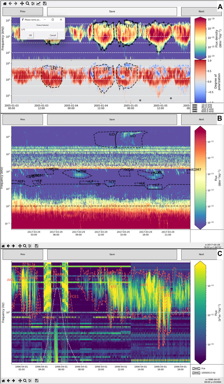
FIGURE 1. Examples of plots from the SPACE labelling Tool. Panel (A) displays Cassini/RPWS (Radio and Plasma Waves Science Gurnett et al., 2004) data (Lamy et al., 2008, 2009). The two panels show Intensity and Polarization data, respectively. At the top right of the top panel one can see a polygon that has just been drawn, with the window for naming the feature appearing at the top left of the graphics window. Other features have already been labelled, and appear in both intensity and polarisation views, with their names overlaid. The data displays in panel (B) are the estimated flux density (Louis et al., 2021a,c) from Juno/Waves measurements (Kurth et al., 2017), with the Louis et al. (2021b) catalogue overlaid. Panel (C) displays observations of Polar/PWI instrument (Gurnett et al., 1995) with the Smith et al. (2022) catalogue overlaid. The horizontal dashed-white line shows an example of the use of the -g [FREQUENCY GUIDE [FREQUENCY GUIDE ...]] option. The variable dashed-white line show that the tool is also able to read a 1D table from the CDF file (provided that this has been specified in the configuration file).
Listing 3: System-wide command to run the space labelling tool - see Section 2.2.2 for more details on the -options.
Users may select any number of the measurement types present in the file (e.g., polarisation, flux and/or power), and view them all tiled on the screen. For example, Figure 1A displays Cassini Flux and Polarization radio data, while Figure 1B only display Juno Flux radio data. Users can then click to select polygonal regions of the observation to label as features (top panel of Figure 1A). To close the polygon, users should click on the first drawn vertex of the polygon. Once done, a window pops up and ask to name the drawn feature appropriately (see top panel of Figure 1A). Features labelled in one view (e.g., intensity) appear simultaneously on the other views once they have been named (see bottom panel of Figure 1A), allowing users to easily see how a feature presents in multiple measurement types.
Once a region has been labelled, a user can pan their viewing window back and forth through the time range within the dataset by clicking on the Prev or Next buttons (see Figure 1), with an overlap applied between each view in order to facilitate labelling features that lie on the edge of a window. Once finished, the labelled regions can be saved as a TFCat (Time-Frequency Catalogue) formatted JSON2 file (Cecconi et al., 2022, this issue) by clicking on the Save button, and used later. If a user re-opens the same data file, or another data file with the same naming structure (e.g., observations_20180601_v02.cdf and observations_20180602_v02.cdf) saved features from previous sessions will be pre-loaded (see Figure 1).
Full usage documentation is available on the GitHub repository of the code (Louis et al., 2022) and directly at https://space-labelling-tool.readthedocs.io.
2.2.1 Procedure
When the code first opens a datafile, it compares the columns within to a selection of pre-made (and user-creatable) ‘configuration’ files for each type of input file (e.g., CDF, HDF5). Each describes a file in terms of the column names within it, and provides metadata for use in the tool - units and display names, and scaling factors that can be applied to change data stored in one unit into data viewed in another. If the data are in an unspecified format, the code will prompt the user to create a configuration file (see Section 2.2.3). Alternatively, if their data fit multiple configuration files, they will be prompted to select which they want to use (see Section 2.2.2).
Once a configuration has been determined, the code parses the observations and may re-bin the time into a coarser resolution in order to improve performance, taking the average of measurements in the new larger bins. It can also rescale the frequency data into evenly-spaced logarithmic bins between the minimum and maximum bins in the original data, as some data files have non-monotonic bin structures. When altering the frequency bins, measurements are logarithmically interpolated between the readings on the previous scale. Default adjustments can be defined in configuration files for file types, and may be over-ridden by command-line arguments to the tool. The parsed and adjusted data are then re-saved as a compressed HDF5 file, reducing both the size of the data and time to access.
The pre-processed data are then displayed to the screen using MatPlotLib (Hunter, 2007), in a window the size of the user’s initial time range. The dynamic range of the data is constrained to improve visibility of features; displaying, by default, the 5th-95th quantiles of the signal for each measurement (to prevent anomalously low or high values overly-compressing the ranges of interest, reducing the ability to discern features). GUI buttons allow users to pan between time windows of equivalent size - with each window will overlap the previous window by 25% in the direction of travel. Features can then be defined by drawing polygons on the time window using the MatPlotLib Polygon Selector widget. There are the detailed interactive components of the MatPlotLib window:
• Measurements: Each panel displays a measurement, with name, scale and units on the right. Features can be drawn by clicking to add coordinates, and completed by clicking on the first coordinate added again. The vertices of the polygon can be modified before completed the polygon:
• Hold the ctrl key and click and drag a vertex to reposition it before the polygon has been completed.
• Hold the shift key and click and drag anywhere in the axes to move all vertices.
• Press the esc key to start a new polygon.
Once selected, a feature can be named (see Figure 1A). Features can be selected on any pane, and will be mirrored on all other panes.
• Prev/Next buttons: These move through the data by an amount equal to the width of time range selected. This will also overlap 1/4 of the current window as ‘padding’.
• Save button: This will save any features to TFcat JSON format, as catalogue_OBSERVER_NAME.json.
• Check boxes: If the option -g [FREQUENCY_GUIDE [FREQUENCY_GUIDE ...]] has been enabled by the users (e.g., fixed frequency lines in Figures 1A,C), or if a 1D variable is contained in the input data and configuration files (e.g., Fce Figure 1C) check boxes will appear in the lower right hand corner of the figure to make the white dotted lines appear or disappear.
Once finished, you can save and then close the figure using the normal close button.
2.2.2 Options
The user must specify the path to the file they want to visualise (or ‘first’ file in a collection, e.g., of CDF files), along with the start and end dates of their initial viewing window, in ISO year-month-day hour:minute:second format (e.g., 2018-06-12 18:00:01). However, there are further options available:
• -f FREQUENCY_BINS: Rescales the data to this many evenly-spaced logarithmic bins. Overrides any default set in the configuration files.
• -t MINIMUM_TIME_BIN: Rebins the data to time bins of this size, if it is currently more finely binned. The bin size need to be given in second.
• -s SPACECRAFT: Specifies the name of the spacecraft configuration file to use, if multiple describe the datafile the user has provided.
• -fig_size FIGURE_SIZE FIGURE_SIZE: x and y dimension of the matplotlib figure (by default: 15 9).
• -frac_dyn_range FRAC_MIN FRAC_MAX: Defines the dynamic range of the colour bar in the visualisation, as a fraction of the distribution of values in the data file. This must be numbers between 0 and 1. Default values are 0.05 and 0.95 (the 5th-95th quantiles of the displayed signal).
• -cmap CMAP: The name of the color map that will be used for the intensity plot (by default: viridis).
• -cfeatures CFEATURES: The name of the colour for the saved features of interest polygons (by default: tomato).
• -thickness_features TFEATURES: The thickness value for the saved features of interest polygons (by default: 2).
• -size_features_name SFEATURESNAME: The font size for the name of the saved features of interest polygons (by default: 14).
• -g [FREQUENCY_GUIDE [FREQUENCY_GUIDE ...]]: Draws horizontal line(s) on the visualisation at these specified frequencies to aid in interpretation of the plot.Values must be in the same units as the data.Lines can be toggled using check boxes.
• –not_verbose: If not_verbose is called, the debug log will not be printed. By default: verbose mode.
2.2.3 Input formats
The code is designed to cope with input files in a variety of file formats and column formats by use of configuration files, several of which are pre-provided. HDF5 input files require at least three datasets, corresponding to observation time (floats, in MJD), frequency range (floats, in any arbitrary unit) and at least one measurement, stored with frequency as the rows and observation as the columns. The names and units for each measurement (in LaTeX form) must be provided in a configuration file, in easily-editable JSON format. The appropriate configuration files are automatically-selected by the code from those available - making it easy to work with HDF5 files from a variety of collaborators with arbitrary naming schemes.
CDF files in NASA format are more structured, and can be read in either singly or as a collection, combining all files in the directory matching the naming scheme [...]_YYYMMDD_[...].cdf into a single pre-processed data file. As with the HDF5 files, CDF files must contain a frequency attribute (floats, in any arbitrary unit) and a time attribute (either in TT_2000 or CDF_EPOCH format, which is parsed using Astropy, Price-Whelan et al., 2018) and at least one measurement, stored with frequency as the rows and observation as the columns.
The code can easily be expanded to ingest other file formats (see Section 2.3.2).
2.3 Structure
2.3.1 ‘Model-View-Presenter’ architecture
The code is designed using a standard object-oriented ‘Model-View-Presenter’ architecture, with strong separation between the data input and management, and the visualisation. This allows for easy development of both new input file-types (see Section 2.3.2) and pre-processing options, and alternative GUI front-ends and settings (see Section 5 for suggested development building on top of this flexibility). A generic ‘Presenter’ controls the logic of the program, and feeds data from the data models to the selected GUI view, and requests from the GUI for changes to the data models. Either the ‘View’ or ‘Model’ can be easily interchanged as long as they conform to the API expected by the ‘Presenter’.
Full development documentation is available on the GitHub repository of the code (Louis et al., 2022) and directly at https://space-labelling-tool.readthedocs.io.
2.3.2 Addition of new input formats
New input formats can be easily added by extending the base DataSet class included in the code. A developer only needs to define the routines for inputting the data from file; the code will then handle pre-processing and data access.
3 History of the code
The first version of the labelling code was developed in IDL by P. Zarka. It allowed users to read data from an IDL saveset (sav format), draw polygons around features of interest and label them. However, this IDL version had to be adapted to each new dataset. This code has been used to build many catalogues based on different observers (such as the Nançay Decameter Array (NDA) ground-based radio telescope (Marques et al., 2017), or the Cassini (Zarka et al., 2021) or Juno (Louis et al., 2021c,b) spacecraft).
The second version of the labelling tool was written in Python and was the first to be officially released (Empey et al., 2021). This version allowed to automatically read any dataset in sav or cdf format, based on the information requested from users from the terminal. The other main improvements compared to the previous version were the number of vertices in the polygons (unlimited) and the possibility to modify the vertices position during the polygon drawing (using the Matplotlib’s Polygon Selector widget), as well as the production of the catalogue directly in TFCat format.
The current version (Louis et al., 2022) brings a large number of improvements, both in terms of architecture, usability and ergonomics, which are described in the previous sections.
The SPACE tool has also joined the MASER service (Cecconi et al., 2020).
4 Applications
Once a catalogue has been produced, it can also be displayed using the SPACE labelling Tool (see Figure 1 or the Autoplot Software (Faden et al., 2010). For an example, the reader is invited to visit the web page https://doi.org/10.25935/nhb2-wy29 where an autoplot template file is given to display the Juno data (Louis et al., 2021a) and the Louis et al. (2021b) catalogue overlaid in autoplot. See Cecconi et al. (2022, this issue) for more information about the display of a Catalogue using Autoplot. The catalogue can be used to study the different components of the radio emission spectrum, e.g. as done by Louis et al. (2021c), where the data can then be automatically selected using the catalogue via a mask or an inverse-mask. In the case presented in Figure 1, not every type of emission is labelled, but in each frequency range (kilometric or hectometric) only one radio component remains. We can then study the components one by one [e.g., their latitudinal distribution, as in Louis et al. (2021c), their distribution as a function of observer’s or Sun’s longitude, as in Zarka et al. (2021), or their distribution versus observer’s longitude and satellite (Io) phase as in Marques et al. (2017)].
With the SPACE labelling Tool, we are also providing some useful routines to use the catalogue3.
These catalogues can also then be used to train machine learning algorithm to detect automatically the radio emissions in past (Cassini, NDA) or future observation (such as Juno, JUICE, NDA).
5 Limitations and future work
The code is ready for distribution and use, but has some technical limitations. Potential works to address those limitations, and avenues of future development, are:
• Performance: The MatPlotLib-based front-end can struggle when provided with especially high resolutions of data, or over large time windows. Rebinning features exist to mitigate this, but an alternative rendering framework could be employed (e.g., datashader4), and/or the performance of the interactive front-end components could be improved if re-implemented in a more performant framework [e.g., Plotly Inc. (2015)].
• Scalability: The code loads all the data provided into memory at launch, limiting its applicability for large datasets. Whilst this can be mitigated by the feature to allow appending to TFCat files created by data files sharing filename formats, a ‘deferred load’ approach would be better. This would be best accomplished using the Dask and XArray libraries (Dask Development Team, 2016; Hoyer and Hamman, 2017).
• Configurations: The code depends heavily on pre-written configuration files, and can prompt users to create missing ones - but does not yet contain a ‘wizard’ or automatic walkthrough to aid users in creating them.
• Platform: Run the SPACE labelling tool in a notebook (launch on Binder).
• Catalogue integration: The modular format of the code would make it possible to create ‘dataset’ types that access and download data directly from online catalogues, maintaining local caches.
Data availability statement
The code of the SPACE labelling Tool is open-source and freely available on github (Louis et al., 2022). The Cassini/RPWS dataset displayed in Figure 1A, produced by Lamy et al. (2008) is available at https: //doi.org/10.25935/ZKXB-6C84 (Lamy et al., 2009). The Juno/Waves dataset displayed in Figure 1B, produced by Louis et al. (2021c), is accessible at https://doi.org/10.25935/6jg4-mk86 (Louis et al., 2021a), and the catalogue can be download at https://doi.org/10.25935/ nhb2-wy29 (Louis et al., 2021b). The Polar/PWI dataset displayed in Figure 1C is accessible through the CDAWeb at https://cdaweb.gsfc.nasa.gov/pub/data/polar/pwi/.
Author contributions
CL and CJ led the development of the SPACE Labelling Tool. CL wrote the paper and worked on the development of the code. PZ developed the first IDL version of the code. AE developed the first python version of the code. SM worked on the development of the second version of the code. SWM developed the current version of the code. EO tested the different versions of the code, and gave inputs to the developers of the code. AB helped run the code on a virtual machine environment, and made changes on the plotting functions to the latest version of the code. AB helped run the code on a virtual machine environment, and made changes on the plotting functions to the latest version of the code. KS added features to the latest version of the code. EO, AB, and KS wrote useful routines to read, modify and use the output catalogue. BC led the TFCat format of the catalogues. All the co-authors have contributed to the writing of the paper.
Funding
CL’s, CJ’s, EO’s, and AE’s work at the Dublin Institute for Advanced Studies was funded by Science Foundation Ireland Grant 18/FRL/6199. SWM’s work at the University of Southampton Research Software Group was funded by a grant via the Alan Turing Institute. KS’s work at the Dublin Institute for Advanced Studies was funded by a 2022 SCOSTEP/PRESTO Grant. The Europlanet 2024 Research Infrastructure project has received funding from the European Union’s Horizon 2020 research and innovation programme under grant agreement No 871149.
Acknowledgments
CL thanks A. Loh and S. Lion for their very helpful comments on the development phase of the code. CL also gives special thanks to R. Prangée for finding errors that no one had seen.
Conflict of interest
The authors declare that the research was conducted in the absence of any commercial or financial relationships that could be construed as a potential conflict of interest.
Publisher’s note
All claims expressed in this article are solely those of the authors and do not necessarily represent those of their affiliated organizations, or those of the publisher, the editors and the reviewers. Any product that may be evaluated in this article, or claim that may be made by its manufacturer, is not guaranteed or endorsed by the publisher.
Footnotes
1https://pypi.org/project/SPACE-labelling-tool/
3https://github.com/elodwyer1/Functions-for-SPACE-Labelling-Tool
References
Bonnin, X., Hoang, S., and Maksimovic, M. (2008). The directivity of solar type III bursts at hectometer and kilometer wavelengths: Wind-Ulysses observations. Astronomy Astrophysic 489, 419–427. doi:10.1051/0004-6361:200809777
Cecconi, B., Loh, A., Sidaner, P. L., Savalle, R., Bonnin, X., Nguyen, Q. N., et al. (2020). Maser: A science ready toolbox for low frequency radio Astronomy. Data Sci. J. 19, 1062. doi:10.5334/dsj-2020-012
Cecconi, B., Louis, C. K., Bonnin, X., Loh, A., and Taylor, M. B. (2022). TFCat (Time-Frequency catalogue): JSON implementation and Python library. Frontiers in astronomy and space sciences. This issue.
Dask Development Team (2016). Dask: Library for dynamic task scheduling. https://dask.org
Empey, A., Louis, C. K., and Jackman, C. M. (2021). SPACE labelling tool. version 1.1.0. [Code]. doi:10.5281/zenodo.5636922
Faden, J. B., Weigel, R. S., and Merka, J., (2010). Autoplot: A browser for scientific data on the web. Earth Sci. Inf. 3, 41–49. doi:10.1007/s12145-010-0049-0
Fogg, A. R., Jackman, C. M., Waters, J. E., Bonnin, X., Lamy, L., Cecconi, B., et al. (2022). Wind/WAVES observations of auroral kilometric radiation: Automated burst detection and terrestrial solar Wind - magnetosphere coupling effects. JGR. Space Phys. 127, e30209. doi:10.1029/2021JA030209
Gurnett, D. A., Kurth, W. S., Kirchner, D. L., Hospodarsky, G. B., Averkamp, T. F., Zarka, P., et al. (2004). The Cassini radio and plasma wave investigation. Space Sci. Rev. 114, 395–463. doi:10.1007/s11214-004-1434-0
Gurnett, D. A., Persoon, A. M., Randall, R. F., Odem, D. L., Remington, S. L., Averkamp, T. F., et al. (1995). The polar plasma wave instrument. Space Sci. Rev. 71, 597–622. doi:10.1007/bf00751343
Hoyer, S., and Hamman, J. (2017). xarray: N-D labeled arrays and datasets in Python. J. Open Res. Softw. 5, 10. doi:10.5334/jors.148
Hunter, J. D. (2007). Matplotlib: A 2d graphics environment. Comput. Sci. Eng. 9, 90–95. doi:10.1109/MCSE.2007.55
Kurth, W. S., Hospodarsky, G. B., Kirchner, D. L., Mokrzycki, B. T., Averkamp, T. F., Robison, W. T., et al. (2017). The Juno waves investigation. Space Sci. Rev. 213, 347–392. doi:10.1007/s11214-017-0396-y
Lamy, L., Cecconi, B., and Zarka, P. (2009). Cassini/RPWS/HFR LESIA/kronos SKR data collection. Version 1.0. [Data set]. doi:10.25935/ZKXB-6C84
Lamy, L. (2017). “The saturnian kilometric radiation before the Cassini grand finale,” in Planetary radio emissions (PRE-VIII). Editors G. Fischer, G. Mann, and M. Panchenko, (Vienna: Austrian Academy of Sciences Press). 455–466. doi:10.1553/PRE8s455
Lamy, L., Zarka, P., Cecconi, B., Prangé, R., Kurth, W. S., and Gurnett, D. A. (2008). Saturn kilometric radiation: Average and statistical properties. J. Geophys. Res. 113, A07201. doi:10.1029/2007JA012900
Leblanc, Y. (2020a). A catalogue of Jovian decametric radio observations from January 1978 to December 1979. Digitised version. [Data set]. doi:10.25935/GXZF-ZT33
Leblanc, Y. (2020b). A catalogue of Jovian decametric radio observations from January 1982 to December 1984. Digitised version. Data set. doi:10.25935/403B-VA51
Leblanc, Y. (2020c). A catalogue of Jovian decametric radio observations from January 1985 to December 1987. Digitised version. [Data set]. doi:10.25935/gh59-py87
Leblanc, Y. (2020d). A catalogue of Jovian decametric radio observations from January 1988 to December 1990. Digitised version. [Data set]. doi:10.25935/cmqb-jj10
Leblanc, Y. (2020e). A catalogue of Jovian radio observations from January 1980 to December 1981. Digitised version. [Data set]. doi:10.25935/RAS0-ER93
Louis, C. K., Jackman, C. M., Mangham, S. W., Smith, K. D., O’Dwyer, E., Empey, A., et al. (2022). SPACE labelling tool. Version 2.0.0. [Code]. doi:10.5281/zenodo.6886528
Louis, C. K., Zarka, P., and Cecconi, B. (2021a). Juno/Waves estimated flux density Collection. Version 1.0. doi:10.25935/6jg4-mk86
Louis, C. K., Zarka, P., Cecconi, B., and Kurth, W. S. (2021b). Catalogue of Jupiter radio emissions identified in the Juno/Waves observations. Version 1.0. doi:10.25935/nhb2-wy29
Louis, C. K., Zarka, P., Dabidin, K., Lampson, P. A., Magalhães, F. P., Boudouma, A., et al. (2021c). Latitudinal beaming of jupiter’s radio emissions from juno/waves flux density measurements. JGR. Space Phys. 126, e29435. doi:10.1029/2021JA029435
Marques, M. S., Zarka, P., Echer, E., Ryabov, V. B., Alves, M. V., Denis, L., et al. (2017). Statistical analysis of 26 yr of observations of decametric radio emissions from Jupiter. Astron. Astrophys. 604, A17. doi:10.1051/0004-6361/201630025
Plotly Inc (2015). Collaborative data science. https://plot.ly
Price-Whelan, A. M., Sipőcz, B., Günther, H., Lim, P., Crawford, S., Conseil, S., et al. (2018). The astropy project: Building an open-science project and status of the v2. 0 core package. Astronomical J. 156, 123. doi:10.3847/1538-3881/aabc4f
Smith, K. D., Louis, C. K., Jackman, C. M., Fogg, A. R., O’Dwyer, E., Waters, J. E., et al. (2022). Catalogue of Auroral Kilometric Radiations (AKR) observed by the Polar spacecraft (1.1). Zenodo. doi:10.5281/zenodo.7235986
Taubenschuss, U., Leisner, J. S., Fischer, G., Gurnett, D. A., and Nemec, F. (2011). “Saturnian low-frequency drifting radio bursts: Statistical properties and polarization,” in Planetary, solar and heliospheric radio emissions (PRE VII). Editors H. O. Rucker, W. S. Kurth, P. Louarn, and G. Fischer (Vienna: Austrian Academy of Sciences Press), 115–123.
Waters, J. E., Jackman, C. M., Lamy, L., Cecconi, B., Whiter, D. K., Bonnin, X., et al. (2021). Empirical selection of auroral kilometric radiation during a multipoint remote observation with Wind and Cassini. JGR. Space Phys. 126, e29425. doi:10.1029/2021JA029425
Ye, S. Y., Fischer, G., Menietti, J. D., Wang, Z., Gurnett, D. A., and Kurth, W. S. (2011). “An overview of Saturn narrowband radio emissions observed by Cassini RPWS,” in Planetary, solar and heliospheric radio emissions (PRE VII). Editors H. O. Rucker, W. S. Kurth, P. Louarn, and G. Fischer. (Vienna: Austrian Academy of Sciences Press), 99–113.
Keywords: python tools, labelling tool, planetary radio emission, solar radio emission, jupiter, saturn, earth, sun
Citation: Louis C, Jackman C, Mangham S, Smith K, O’Dwyer E, Empey A, Cecconi B, Boudouma A, Zarka P and Maloney S (2022) The “SPectrogram Analysis and Cataloguing Environment” (SPACE) labelling tool. Front. Astron. Space Sci. 9:1001166. doi: 10.3389/fspas.2022.1001166
Received: 22 July 2022; Accepted: 21 October 2022;
Published: 14 November 2022.
Edited by:
K.-Michael Aye, Freie Universität Berlin, GermanyReviewed by:
Mario D'Amore, German Aerospace Center (DLR), GermanyReinaldo Roberto Rosa, National Institute of Space Research (INPE), Brazil
Copyright © 2022 Louis, Jackman, Mangham, Smith, O’Dwyer, Empey, Cecconi, Boudouma, Zarka and Maloney. This is an open-access article distributed under the terms of the Creative Commons Attribution License (CC BY). The use, distribution or reproduction in other forums is permitted, provided the original author(s) and the copyright owner(s) are credited and that the original publication in this journal is cited, in accordance with accepted academic practice. No use, distribution or reproduction is permitted which does not comply with these terms.
*Correspondence: Corentin Louis, Y29yZW50aW4ubG91aXNAZGlhcy5pZQ==
†ORCID: Corentin Louis, orcid.org/0000-0002-9552-8822; Caitriona Jackman, orcid.org/0000-0003-0635-7361; Sam Mangham, orcid.org/0000-0001-7511-5652; Kevin Smith, orcid.org/0000-0002-9274-8715; Elizabeth O’Dwyer, orcid.org/0000-0003-3780-4953; Aaron Empey, orcid.org/0000-0001-6448-7178; Baptiste Cecconi, orcid.org/0000-0001-7915-5571; Adam Boudouma, orcid.org/0000-0002-8693-9398; Philippe Zarka, orcid.org/0000-0003-1672-9878; Shane Maloney, orcid.org/0000-0002-4715-1805