Non-Linear Damping of Surface Alfvén Waves Due to Uniturbulence

This investigation is concerned with uniturbulence associated with surface Alfvén waves that exist in a Cartesian equilibrium model with a constant magnetic field and a piece-wise constant density. The surface where the equilibrium density changes in a discontinuous manner are the source of surface Alfvén waves. These surface Alfvén waves create uniturbulence because of the variation of the density across the background magnetic field. The damping of the surface Alfvén waves due to uniturbulence is determined using the Elsässer formulation. Analytical expressions for the wave energy density, the energy cascade, and the damping time are derived. The study of uniturbulence due to surface Alfvén waves is inspired by the observation that (the fundamental radial mode of) kink waves behave similarly to surface Alfvén waves. The results for this relatively simple case of surface Alfvén waves can help us understand the more complicated case of kink waves in cylinders. We perform a series of 3D ideal MHD simulations for a numerical demonstration of the non-linearly self-cascading model of unidirectional surface Alfvén waves using the code MPI-AMRVAC. We show that surface Alfvén waves damping time in the numerical simulations follows well our analytical prediction for that quantity. Analytical theory and the simulations show that the damping time is inversely proportional to the amplitude of the surface Alfvén waves and the density contrast. This unidirectional cascade may play a role in heating the coronal plasma.

1 Introduction

Magnetohydrodynamic (MHD) turbulence is one of the most important physical processes at large scales in plasma, as many astrophysical and laboratory plasmas are in a turbulent state (Goldstein et al., 1995; Biskamp, 2003; Bruno and Carbone, 2005; Cranmer et al., 2007). It is generally understood that the role of the magnetic field is significant under certain situations. Turbulence efficiently helps in the mixing and transport of energy and matter across scales as it cascades from large scales to small scales, whereas the dissipation only becomes essential in the smallest scales, i.e., Kolmogorov scales. Therefore, turbulence is believed to be at least partly responsible for heating the solar corona and accelerating the solar wind (Tu and Marsch, 1995; Verdini et al., 2009). Furthermore, Kolmogorov (1941) revealed that in fluid turbulence, the energy cascade to smaller scales is independent from the scale, resulting in a power-law behavior in the so-called inertial range. After this range, turbulent eddies transfer to the dissipative range, in a sense that heating occurs as the fluctuations are damped. The study of MHD turbulence began with Iroshnikov (1964), and Kraichnan (1965), who generalized Kolmogorov’s theory to the presence of magnetic field and its stabilizing influence.

It is widely believed that convective motions in the photosphere generate waves propagating away from the sun (Heinemann and Olbert, 1980; Heyvaerts and Priest, 1983; Matthaeus et al., 2003; Perez and Chandran, 2013). Waves that are propagating upwards continuously reflect towards the Sun due to the gravitational stratification of the plasma, which causes the Alfvén speed to vary along the magnetic field lines. The reflected waves interact with waves propagating upwards. This process creates the turbulent cascade and leads to energy dissipation (Matthaeus et al., 1999; Van Doorsselaere et al., 2020b). This process has also been modeled extensively in numerical experiments (Suzuki and Inutsuka, 2005; Rappazzo et al., 2008; van Ballegooijen et al., 2011; Shoda and Yokoyama, 2018). The large majority of those considered either a completely homogeneous background or only inhomogeneity along the magnetic field in a setting of incompressible MHD. In incompressible MHD, these counterpropagating waves are conveniently described by Elsässer variables, ${\vec{Z}}^{\pm }=\vec{v}\pm \vec{B}/\sqrt{\mu \rho }$, where $\vec{v}$ is the velocity of the plasma, $\vec{B}$ is the magnetic field, μ and ρ are the magnetic permeability and density. Many authors use these variables to distinguish inward ( + ) and outward ( − ) propagating Alfvén waves. They are thought to interact non-linearly to generate an energy cascade, and their nature helps us understand more about the MHD turbulence cascade mechanism.

Observations showed that transverse waves are critical for transferring energy from the photosphere to the solar corona, where research efforts have mainly focused on standing and propagating kink waves (De Pontieu et al., 2007; Tomczyk et al., 2007; Anfinogentov et al., 2015; Kohutova et al., 2020). Furthermore, transverse standing waves have been extensively studied numerically, where it was revealed that standing transverse oscillations are the decisive point of developing Kelvin-Helmholtz instability (KHI) non-linearly (Terradas et al., 2008; Antolin et al., 2016). Lately, Van Doorsselaere et al. (2021) developed a nonlinear damping model for standing kink waves and showed that the damping time is inversely proportional to the oscillation amplitude, where they also found a notable match with the observation (Nechaeva et al., 2019). Compared to standing transverse oscillations, propagating kink waves have received little attention (Thurgood et al., 2014; Morton et al., 2021).

State of the art in turbulence generation in MHD is the phenomenology of the counterpropagating Alfvén waves. In other words, for turbulence to be generated by waves, one needs waves that collide. According to the currently accepted phenomenology, turbulence generated by MHD waves relies on the counterpropagating waves’ collision. In case when the wave-packet propagates parallel to the magnetic field with the inhomogeneity across the field, it causes the initial Alfvénic wave-package to self-deform nonlinearly as it propagates, cascading to smaller scales. This can act as an additional channel towards a turbulent cascade, thereby enhancing the dissipation rate and increasing heating (Van Doorsselaere et al., 2020b). In recent years, it was realized that unidirectionally (in the same direction) propagating waves also generate turbulence when there is inhomogeneity across the field (Magyar et al., 2017; 2019a). These unidirectional waves carry both Elsässer variables. It indicates that ${\vec{Z}}^{\pm }$ cannot be longer separated and associated with waves propagating in one direction and the other. It also means that one unidirectional wave has to be described by both these Elsässer variables propagating in one direction. Consequently, the nonlinear advective term ${\vec{Z}}^{\mp }\cdot \nabla {\vec{Z}}^{\pm }$ is nonzero, leading to the cascade. In an inhomogeneous plasma, it can be nonzero also for waves propagating only in one direction. Thus, there is no need for reflections to generate counterpropagating waves. This phenomenon was first introduced by Magyar et al. (2017) and has been named uniturbulence. Such turbulence can exist in open magnetic field regions and may play a role in heating the coronal plasma because the additional energy cascade term is included (Van Doorsselaere et al., 2020a).

In this paper, we mainly study the surface Alfvén waves. Surface Alfvén waves are MHD waves that appear at the discontinuity and have zero vorticity everywhere except at the interface (Goossens et al., 2012). Moreover, Wentzel (1979a) mentioned that the phase speed of these waves ranges between the internal and external Alfvén phase velocities. Surface Alfvén waves propagate unidirectionally with no backward reflections. Surface Alfvén waves are waves propagating in one direction, suggesting that both Elsässer variables represent surface Alfvén waves and are connected and co-propagating. These waves are indeed no longer pure Alfvén waves. The inward or outward Elsässer variables can separate only pure Alfvén waves in an incompressible medium. As a result, they must be characterized by both Elsässer variables. Unidirectional surface Alfvén waves have also been extensively discussed in the paper by Magyar et al. (2019b).

Ionson (1978) was the first to consider resonant absorption for heating solar coronal loops when it comes to dissipation. Ionson studied surface Alfvén waves in a Cartesian system. He applied the method of Sedláček (1971) to solve the dispersion relation and obtained the damping rate. That was pointed out by Wentzel (1979b). Wentzel dealt with both the Alfvén and the slow resonance in Cartesian geometry. Also, it gives an enlightening discussion of the Sedlacek procedure.

Hollweg and Yang (1988) studied the damping of compressible MHD waves at thin surfaces in Cartesian geometry. They used the approximation that the perturbation of pressure is constant in the non-uniform layer. Their numerical example applied their analytical result to cylindrical loops using the simple ad hoc transformation from Cartesian to cylindrical geometry k_z = π/L, k_y = 1/R, m = 1. They concluded that kink waves would undergo fast damping due to resonant absorption. The damping due to resonant absorption is much faster than the damping due to viscosity and resistivity. This is the first theoretical result on the fast damping of kink waves on coronal loops.

Expressions for the damping rate due to resonant absorption are given by Goossens et al. (1992) for non-axisymmetric MHD waves. For m = 1, the waves are kink waves. Goossens et al. (1992) confirm the results of Hollweg and Yang (1988). Also, the simple Hollweg and Yang (1988) transformation from a Cartesian to a cylindrical system for a straight field gives correct results. Ruderman and Roberts (2002) showed that two-time scales are involved in resonant absorption and recovered Goossens et al. (1992). Recently, Antolin and Van Doorsselaere (2019) studied the effect of resonant absorption for the generation of the KHI, where they pointed out that it plays a crucial role in exciting and developing the transverse wave-induced KHI rolls in the loop.

This paper investigates uniturbulence associated with surface Alfvén waves that exist in a Cartesian equilibrium model with a constant magnetic field and a piece-wise constant density. The surface where the equilibrium density changes in a discontinuous manner is the source of surface Alfvén waves. These surface Alfvén waves create uniturbulence because of the variation of the density across the background magnetic field. The damping of surface Alfvén waves due to uniturbulence is determined using the Elsasser formulation. We are inspired by the work of Van Doorsselaere et al. (2020a). Van Doorsselaere et al. (2020a) studied the energy dissipation for propagating kink waves in cylindrical plasma configurations and derived analytical expressions for the timescale of the energy cascade. The main goal of the present paper is to support the results by Van Doorsselaere et al. (2020a) by using their scheme to obtain analytical and numerical results for surface Alfvén waves on a simple Cartesian equilibrium configuration. Section 2 presents the analytical model for uniturbulence driven by surface Alfvén waves and the resulting damping of the surface Alfvén waves. The numerical scheme is presented in Section 3. Results are presented and analyzed in Section 4. Finally, conclusions are given in Section 5.

2 Analytical Model for Uniturbulent Damping of Surface Alfvén Waves

Two preliminary analyses were undertaken. First, we repeat the calculation of Van Doorsselaere et al. (2020a) in Cartesian coordinates, in contrast to their analytical model of the nonlinear evolution of kink waves in cylindrical geometry. Van Doorsselaere et al. (2020a) described transverse kink waves by Bessel functions, but we derive classic results for the surface Alfvén waves (Section 2.1). Nevertheless, we use similar approach for calculating the wave energy density (Section 2.3) and the energy cascade rate (Section 2.4) by using the Elsässer variables (Section 2.2). Secondly, we derive the damping time scale in a long-wavelength limit (Section 2.5).

2.1 Governing Equations and Surface Alfvén Waves

We use the ideal incompressible MHD equations,

$\begin{array}{ccc}\hfill \nabla \cdot \vec{v}=0,& \hfill & \hfill \end{array}(1)$

$\begin{array}{ccc}\hfill \rho \frac{\partial \vec{v}}{\partial t}+\rho \vec{v}\cdot \nabla \vec{v}=-\nabla p+\frac{1}{\mu }(\nabla \times \vec{B})\times \vec{B},& \hfill & \hfill \end{array}(2)$

$\begin{array}{ccc}\hfill \frac{\partial \vec{B}}{\partial t}=\nabla \times (\vec{v}\times \vec{B}),& \hfill & \hfill \end{array}(3)$

where $\vec{v}$ denotes the velocity field of the plasma, $\vec{B}$ is the magnetic field, ρ is the density, μ is the magnetic permeability, and p is the gas pressure.

We consider an equilibrium configuration in a Cartesian coordinate system with a uniform background magnetic field which is directed along with the z axis ($\overrightarrow{B_0}=B_0{\vec{e}}_z$) and no background flow (${\vec{v}}_0=0$). Here and hereafter, we chose a piece-wise constant density (Goossens et al., 2012):

$\rho (x)=\left\{\begin{array}{c}{\rho }_l\text{if}x\le 0,\hfill \\ {\rho }_r\text{if}x>0,\hfill \end{array}\right.(4)$

where ρ_l and ρ_r are constant and ρ_l ≠ ρ_r. We use l and r indices to distinguish the density values on the left and right sides of the interface. As a next step, the incompressible MHD equations have been linearised ($\vec{B}={\vec{B}}_0+{\vec{B}}^{\prime },\vec{v}=0+{\vec{v}}^{\prime },\rho ={\rho }_0+{\rho }^{\prime },p=p_0+p^{\prime }$):

$\begin{array}{ccc}\hfill \nabla \cdot \vec{v}=0,& \hfill & \hfill \\ \hfill {\rho }_0\frac{\partial {\vec{v}}^{\prime }}{\partial t}=-\nabla p^{\prime }+\frac{1}{\mu }({\vec{B}}_0\cdot \nabla ){\vec{B}}^{\prime }-\frac{1}{\mu }\nabla {\vec{B}}_0\cdot {\vec{B}}^{\prime },& \hfill & \hfill \\ \hfill \frac{\partial {\vec{B}}^{\prime }}{\partial t}-({\vec{B}}_0\cdot \nabla ){\vec{v}}^{\prime }=0,& \hfill & \hfill \end{array}$

We take all perturbed quantities proportional to f′ = f(x)  exp(i (k_y y + k_z z − ω t)). We Fourier decompose the perturbation with respect to y, z and t, as the equilibrium quantities are only depending on x. Here f represents the physical variables, ω is the wave frequency and k_y, k_z are the wavenumbers. As a next step, we rewrite the equation in terms of displacement ($\vec{\xi }=d{\vec{v}}^{\prime }/dt$) and total pressure (P′ = p′ + B₀ B_z/μ). Eliminating the variables (ξ_y, ξ_z, ρ₀, B_x, B_y), we can combine the linearized MHD equations into one 2nd order differential equation (ODE). Using the x-component of the equation of motion

$\frac{d{P}^{\prime }}{dx}={\rho }_0({\omega }^2-{\omega }_A^2){\xi }_x,(5)$

where ω_A = k_z V_A and $V_A=B_0/\sqrt{\mu \rho (x)}$. We get a 2nd order ODE for total pressure as follows

${\rho }_0({\omega }^2-{\omega }_A^2)\frac{d}{dx}\left(\frac{1}{{\rho }_0({\omega }^2-{\omega }_A^2)}\frac{d{P}^{\prime }}{dx}\right)={\kappa }^2{P}^{\prime }.(6)$

We introduce the new variable ${\kappa }^2=k_y^2+k_z^2$, which is the wavenumber in the perpendicular direction (i.e., perpendicular to the density interface). We consider the unidirectional magnetic field along the z direction, which allows us to take different Alfvén speeds on the left and the right side. In other words, surface waves can exist only when V_Al ≠ V_Ar (indices l and r denotes left and right side of the density medium, see Eq. 4). Now due to constant quantities in each half-space Eq. 6 simplifies into

$\frac{d^2{P}^{\prime }}{d{x}^2}={\kappa }^2{P}^{\prime },(7)$

The solutions for Eq. 7 are finite at x = ±∞ if and only if

$P^{\prime }(x)=\left\{\begin{array}{c}{P}_l^{\prime }=C_1{e}^{\kappa x},\text{if}x\le 0,\hfill \\ P_r^{\prime }=C_2{e}^{-\kappa x},\text{if}x>0,\hfill \end{array}\right.(8)$

At this point we implement the continuity conditions for total pressure ${\left[P^{\prime }\right]}_{x=0}=0$ and displacement ${\left[{\xi }_x\right]}_{x=0}=0$ at the interface x = 0. The braces denote the difference across the interface. This resulted in C₁ = C₂ = C and the known dispersion relation for surface waves (Ionson, 1978; Wentzel, 1979b; Roberts, 1981) as follows

${\omega }^2=\frac{{\rho }_l{\omega }_{Al}^2+{\rho }_r{\omega }_{Ar}^2}{{\rho }_l+{\rho }_r},(9)$

where ω_Al = k_z V_Al and ω_Ar = k_z V_Ar.

2.2 Elsässer Variables

Now we compute the Elsässer variables for surface Alfvén waves in our setup. We show that surface Alfvén waves carry both Elsässer variables even if they propagate only in one direction (inward or outward). This is in clear contrast to Alfvén waves in uniform plasmas. Therefore, we describe the Elsässer variables for perturbed quantities.

${\vec{Z}}^{\pm }={\vec{v}}^{\prime }\pm \frac{{\vec{B}}^{\prime }}{\sqrt{\mu {\rho }_0}},(10)$

where the Elsässer variables are the well-known combination of flow and Alfvén speed perturbation. In an attempt to calculate the Elsässer variables, we determine the linear variables as follows

$\begin{array}{c}\hfill {\vec{v}}^{\prime }=\frac{d\vec{\xi }}{dt}=\frac{1}{{\rho }_0({\omega }^2-{\omega }_A^2)}\frac{d}{dt}(\nabla P^{\prime }),\\ \hfill {\vec{B}}^{\prime }=B_0\frac{d\vec{\xi }}{dz}=\frac{B_0}{{\rho }_0({\omega }^2-{\omega }_A^2)}\frac{d}{dz}(\nabla P^{\prime }).\end{array}(11)$

Here frequency omega is ω = ω_k given in Eq. 9. For a propagating wave, we take total pressure as P′ = P′(x) cos k_y y  cos(k_z z − ω t), where we take P′(x) as in Eq. 8. P′ is harmonic in time, in y and z directions, as the κ contains both k_y and k_z. We substitute Eq. 11 into Eq. 10 in computing the Elsässer variables as follows

$\begin{array}{ccc}\hfill Z_x^{\pm }=\frac{d{P}^{\prime }(x)}{dx}\frac{\omega \mp {\omega }_A}{{\rho }_0({\omega }^2-{\omega }_A^2)}\cos k_{y}y\sin (k_{z}z-\omega t),& \hfill & \hfill \end{array}(12)$

$\begin{array}{ccc}\hfill Z_y^{\pm }=-P^{\prime }(x)k_y\frac{\omega \mp {\omega }_A}{{\rho }_0({\omega }^2-{\omega }_A^2)}\sin k_{y}y\sin (k_{z}z-\omega t),& \hfill & \hfill \end{array}(13)$

$\begin{array}{ccc}\hfill Z_z^{\pm }=P^{\prime }(x)k_z\frac{\omega \mp {\omega }_A}{{\rho }_0({\omega }^2-{\omega }_A^2)}\cos k_{y}y\cos (k_{z}z-\omega t),& \hfill & \hfill \end{array}(14)$

2.3 Wave Energy Densities

In this section, we derive the evolution of the wave energy densities. With the use of the definition of Elsässer variables, we obtain an expression for wave energy densities.

$\begin{array}{c}\hfill w^{\pm }=\frac{{\rho }_0{({\vec{Z}}^{\pm })}^2}{4}=\frac{{(\omega \mp {\omega }_A)}^2}{4{\rho }_0{({\omega }^2-{\omega }_A^2)}^2}\left[{\left(\frac{\partial P^{\prime }}{\partial x}\right)}^2{\cos }^2{k}_{y}y+P^{\prime 2}{k}_y^2{\sin }^2{k}_{y}y\right]{\sin }^2(k_{z}z-\omega t)+\\ \hfill +\frac{k_z^2{P}^{\prime 2}{(\omega \mp {\omega }_A)}^2}{4{\rho }_0{({\omega }^2-{\omega }_A^2)}^2}{\cos }^2(k_{y}y){\cos }^2(k_{z}z-\omega t).\end{array}(15)$

This can be simplified for the solutions (Eq. 8) in the two regions

$\begin{array}{c}\hfill w_r^{\pm }=\frac{C^2{e}^{-2\kappa x}}{4{\rho }_r{(\omega \pm {\omega }_{Ar})}^2}\left(k_y^2{\sin }^2(k_{z}z-\omega t)+k_z^2{\cos }^2(k_{y}y)\right),\\ \hfill w_l^{\pm }=\frac{C^2{e}^{2\kappa x}}{4{\rho }_l{(\omega \pm {\omega }_{Al})}^2}\left(k_y^2{\sin }^2(k_{z}z-\omega t)+k_z^2{\cos }^2(k_{y}y)\right),\end{array}(16)$

We calculate the energy density averaged over the cross-section and over the period

$⟨w⟩={\int }_{x}dx\frac{k_y}{2\pi }{\int }_0^{2\pi /k_y}dy\frac{\omega }{2\pi }{\int }_0^{2\pi /\omega }wdt,$

When we average over the x direction, we use the variable as a predetermined length L in the transverse direction. The integration in the x direction is from − L to + L

$\langle w_r\rangle =\langle w_r^{+}+w_r^{-}\rangle =\frac{C^2\kappa }{8}\frac{({\omega }^2+{\omega }_{Ar}^2)}{{\rho }_r{({\omega }^2-{\omega }_{Ar}^2)}^2}(1-e^{-2\kappa L}),$

$\langle w_l\rangle =\langle w_l^{+}+w_l^{-}\rangle =\frac{C^2\kappa }{8}\frac{({\omega }^2+{\omega }_{Al}^2)}{{\rho }_l{({\omega }^2-{\omega }_{Al}^2)}^2}(1-e^{-2\kappa L}),$

After taking the average wave energy density for two different regions, we take the sum of ⟨w⟩ = ⟨w_l⟩ + ⟨w_r⟩. We obtain the energy density averaged over the cross-section as follow

$⟨w⟩=\frac{C^2\kappa }{8}\frac{{\rho }_r{({\omega }^2-{\omega }_{Ar}^2)}^2({\omega }^2+{\omega }_{Al}^2)+{\rho }_l{({\omega }^2-{\omega }_{Al}^2)}^2({\omega }^2+{\omega }_{Ar}^2)}{{\rho }_l{\rho }_r{({\omega }^2-{\omega }_{Al}^2)}^2{({\omega }^2-{\omega }_{Ar}^2)}^2}(1-e^{-2\kappa L}),(17)$

By using the dispersion relation (Eq. 9) it simplifies to

$⟨w⟩=\frac{C^2\kappa }{4}\frac{{({\rho }_r+{\rho }_l)}^3{\omega }^2}{{\rho }_r^2{\rho }_l^2{({\omega }_{Al}^2-{\omega }_{Ar}^2)}^2}(1-e^{-2\kappa L}).(18)$

2.4 Energy Dissipation Rate

The energy cascade rate is computed from the non-linear term in the incompressible MHD equations. Following Van Doorsselaere et al. (2020a), the energy dissipation rate for upward and downward surface Alfvén waves can be expressed by using.

${ϵ}^{\pm }={\vec{Z}}^{\mp }\cdot \nabla w^{\pm }(19)$

We find that

${ϵ}_r^{\pm }=\frac{C^3{e}^{-3\kappa x}\cos (k_{y}y)\sin (k_{z}z-\omega t)}{2{\rho }_r^2({\omega }^2-{\omega }_{Ar}^2)(\omega \pm {\omega }_{Ar})}\left[k_z^4{\cos }^2(k_{y}y)+k_y^4{\sin }^2(k_{z}z-\omega t)+2k_y^2{k}_z^2\right],x>0,(20)$

${ϵ}_l^{\pm }=\frac{C^3{e}^{3\kappa x}\cos (k_{y}y)\sin (k_{z}z-\omega t)}{2{\rho }_l^2({\omega }^2-{\omega }_{Al}^2)(\omega \pm {\omega }_{Al})}\left[k_z^4{\cos }^2(k_{y}y)+k_y^4{\sin }^2(k_{z}z-\omega t)+2k_y^2{k}_z^2\right],x\le 0.(21)$

Since there are the third power of a periodic function in the y direction and time, taking the average of Eqs 20, 21 leads to an energy cascade rate of 0. In solar wind Alfvén turbulence model, this zero average in the time domain is avoided by approximating ${\vec{Z}}^{\pm }\cdot \nabla w^{\pm }$ to $\sqrt{{({\vec{Z}}^{\pm })}^2}{w}^{\pm }/L$, where L is the correlation length that defines the perpendicular scales of the wave energy distributions. Van Doorsselaere et al. (2020a) generalized this method and used the root-mean-square approach while averaging over a period and the φ direction. In order to avoid an energy cascade equal to zero, we use the root-mean-square approximation while averaging over the y direction and period.

$⟨ϵ⟩={\int }_{x}dx{\left(\frac{k_y}{2\pi }{\int }_0^{2\pi /k_y}dy\frac{\omega }{2\pi }{\int }_0^{2\pi /\omega }{ϵ}^{2}dt\right)}^{1/2},(22)$

Finally,

$\langle {ϵ}_r\rangle =\langle {ϵ}_r^{+}+{ϵ}_r^{-}\rangle =\frac{\sqrt{2}}{24}\frac{\omega |C^3|}{\kappa }\frac{\sqrt{5k_y^8+24k_y^6{k}_z^2+41k_y^4{k}_z^4+24k_y^2{k}_z^6+5k_z^8}}{{({\omega }^2-{\omega }_{Ar}^2)}^2{\rho }_r^2}(1-e^{-3\kappa L}),(23)$

$\langle {ϵ}_l\rangle =\langle {ϵ}_l^{+}+{ϵ}_l^{-}\rangle =\frac{\sqrt{2}}{24}\frac{\omega |C^3|}{\kappa }\frac{\sqrt{5k_y^8+24k_y^6{k}_z^2+41k_y^4{k}_z^4+24k_y^2{k}_z^6+5k_z^8}}{{({\omega }^2-{\omega }_{Al}^2)}^2{\rho }_l^2}(1-e^{-3\kappa L}),(24)$

Once more we use the dispersion relation to reduce the expression as follows

$⟨ϵ⟩=\frac{\sqrt{2}}{12}\frac{\omega |C^3|}{\kappa }\sqrt{5k_y^8+24k_y^6{k}_z^2+41k_y^4{k}_z^4+24k_y^2{k}_z^6+5k_z^8}\frac{{({\rho }_r+{\rho }_l)}^2}{{\rho }_r^2{\rho }_l^2{({\omega }_{Al}^2-{\omega }_{Ar}^2)}^2}(1-e^{-3\kappa L}),(25)$

Taking the ratio τ = ⟨w⟩/⟨ϵ⟩ and considering L → ∞ we get

$\tau =\frac{3\sqrt{2}}{C}\frac{\omega ({\rho }_r+{\rho }_l)(k_y^2+k_z^2)}{\sqrt{5k_y^8+24k_y^6{k}_z^2+41k_y^4{k}_z^4+24k_y^2{k}_z^6+5k_z^8}}.(26)$

2.5 Long-Wavelength Approximation

We know that in solar corona structure, k_z ≫ k_⊥ (length of the structure is much longer than the length scale in the perpendicular direction), which allows us to acknowledge the long-wavelength limit. In order to simplify the last equation, we consider quasi-perpendicular propagation, also known as the long-wavelength limit. We use this assumption to reduce the complexity of the wavenumber expression. We introduce the new parameter δ = k_z/k_y ≪ 1. Taking the perpendicular component v_y from Eq. 11 yields.

$\frac{v_y}{V_A}\sim \frac{-C}{V_{Ar}}\frac{k_y\omega }{{\rho }_r({\omega }^2-{\omega }_{Ar}^2)},\text{if}x>0$

Considering last expression and rewriting in terms of the density contrast ζ = ρ_r/ρ_l leads Eq. 26 to

$\tau =\frac{3\sqrt{10}}{5V{k}_y}\frac{\zeta +1}{\zeta -1},(27)$

We can see that in an inhomogeneous incompressible MHD, the damping time scale is inversely proportional to the oscillation amplitude V, where for the density contrast, we obtained same relation as was discussed by Van Doorsselaere et al. (2020a). They found a similar expression for damping time in the cylindrical configuration:

$\tau =2\sqrt{5\pi }\frac{R}{V}\frac{\zeta +1}{\zeta -1},(28)$

Here V is the velocity amplitude, and R is the radius of the coronal loop, which in planar geometry R = 1/k_y can be used. Remarkably, the only difference is the factor, which is approximately 4 times smaller. We show that the fundamental radial mode of kink waves in a cylinder behaves very much like a surface Alfvén waves.

We will be able to vary in the simulations the parameters involved in this formula for the damping by the energy cascade. These surface Alfvén waves can be easily numerically modeled, and we can directly compare the energy dissipation rate to this analytical work we derived.

3 Numerical Demonstration of Self-Cascading

In this section, we simulate unidirectional propagating waves as was previously done by Magyar et al. (2019b). We compare our non-linear damping model of the surface Alfvén waves with the series of numerical simulations. Notably, we investigate the dependence on the velocity amplitude of the waves and density contrast to observe if our damping formula is also adequate for the simulation. Moreover, we extend the study of Van Doorsselaere et al. (2020a) and verify their results with the direct numerical simulations of uniturbulence formation in a simple configuration.

3.1 Numerical Setup

3D ideal MHD simulations were run for numerical demonstration of the self-cascading model using the code MPI-AMRVAC (Keppens et al., 2012; Xia et al., 2018). In the simulation, flux schemes were adopted with a five-wave variant, HLLD solver, and Woodward slope limiter. The base grid resolution is chosen as 60 × 60 × 40 in x, y, and z directions, respectively. After applying three-level refinement, the grid resolution becomes 240 × 240 × 160. However, the physical system domain is 0.12 × 0.1 × Z₀, where Z₀ has been changed with the density contrast as in Table 1, and the lower density contrast requires additional length along the z direction due to weaker damping. All the results are presented in code units. We establish the following normalization values of unit velocity = 1.16 × 10⁴ cm/s, unit length = 1 cm, number density = 1 cm⁻³, and unit time = 8.6 × 10⁻⁵s in our code. For a series of simulations the chosen values for amplitudes are V = {0.01, 0.03, 0.06, 0.12, 0.18}, where ζ = 5 considered and similarly we change the density contrast ζ = {1.1, 2, 5, 10, 20} for V = 0.06.

TABLE 1

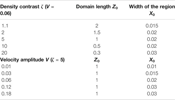
TABLE 1. The table shows different simulations, changing the ζ values for V = 0.06, similarly, different V values for ζ = 5. The chosen domain lengths (Z₀) and analyzed width (X₀) for different simulations illustrate in the last two columns.

We chose simple initial conditions of our model. The following quantities are in code units. Firstly, the straight, homogeneous magnetic field value is B₀ = 1.115 along the z-axis, but this value does not play a significant role. Secondly, we employ a step function of density perpendicular to the magnetic field, which is, in our case, at x = 0, where the density changes discontinuously for ρ_l to ρ_r. In the y and z direction, it does not vary. Moreover, in the simulations, we considered a nearly incompressible regime. The minimum Alfvén speed is V_A ∼ 0.7 and sound speed is V_s ∼ 1.78, resulting in a high plasma β ∼ 4.4. These are significantly greater than our velocity perturbation. Furthermore, in the paper by Magyar et al. (2019b), they considered tests with different plasma beta values (from β ≈ 0.02 to 15), indicating that the dynamics perpendicular to the magnetic field is not very sensitive to its value.

Firstly, we check if the numerical dissipation influences the measured damping time driven by cascade. The higher resolution affects the generation of smaller scales at the interface but leads to almost similar results for the damping time. We run the simulation for V = 0.06 and ζ = 5 case with the 400 × 400 × 240 grid resolution and the damping time is τ ≈ 0.85. The calculated damping time is similar with a lower resolution: τ ≈ 0.85.

3.2 Boundary Conditions

We implement the following boundary conditions: First, at the bottom of the z direction, we take a velocity along the x direction, which varies sinusoidally in y.

$v_x(y,t)=V\cos (\omega t)\sin (k_{y}y).$

According to Magyar et al. (2019b), such a driver will result in uniturbulence in our setup. Here V is the initial velocity amplitude, the frequency of driver is ω = 2 π and the wavenumber chosen for one wavelength in the y direction, k_y = 2 π/0.1.

Second, continuous conditions (Neumann style zero gradient conditions) are taken in the top boundary in the z direction and both x directions for all variables. Third, for the y direction, we used periodic boundary conditions.

4 Results

4.1 Numerical Results

Figures 1, 2 1constitute a set of three-dimensional fluctuations of density change for various initial velocity amplitudes (V) and density contrasts (ζ), respectively. We take snapshots of the cross-section at half of the z domain, with the relevant Z₀ values (Table 1). However, all snapshots were taken at four time period (t = 4.0) except V = 0.18 and ζ = 20. These latter snapshots were taken at t = 2.5 due to the high velocity amplitude or high density contrast numerical simulations becoming unstable for reasons we do not fully understand. In any case, we analyze the first five wavefronts in the remaining text, and the t = 2.5 time is admissible to determine the mean damping time of the first five wavefronts avoiding the instability. In Figure 1 we can see that even at low amplitude, the interface changes its sinusoidal shape and shows effects of non-linearity. Increasing density contrast shows the turbulence and energy cascade loss from large-scale motion to small-scale motion leading to numerical energy dissipation. On the other hand, increasing the amplitude shows that the nonlinear generation of smaller scales is increasing drastically on the density surface, showing evidence of uniturbulence. However, in Figure 2 at ζ = 1.1, we can see that the interface keeps its shape for a more extended time period, showing that uniturbulence is delayed. We can also see that the interface moves with much higher amplitude in higher density contrast regimes due to the significant differences of slow and fast Alfvén speed ($\vec{B}/\sqrt{\mu {\rho }_l}\gg \vec{B}/\sqrt{\mu {\rho }_r}$).

FIGURE 1

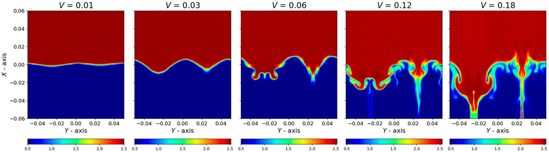
FIGURE 1. Cross-section of density variation at z = 0.5. Plots taken after four driver period for different velocity amplitudes (V = 0.01, 0.03, 0.06, 0.12, 0.18). In all simulations ζ = 5.

FIGURE 2

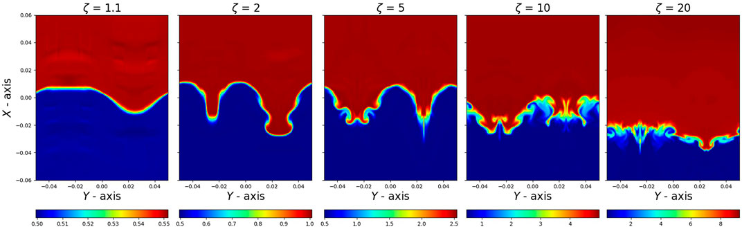
FIGURE 2. Snapshots of evolution of density at half of the z domain according to the table and t = 4. Plots vary for different density contrast ζ = {1.1, 2, 5, 10, 20}, where V = 0.06.

4.2 Analysis and Results

In order to see how the energy transfers to smaller scales in the system, we compute the power spectrum of the velocity field by performing FFT of the v_x component along the y direction (Popescu Braileanu et al., 2021). In particular, we consider the Fourier power at k_y = 2π/0.1 to track the wave’s amplitude in the fundamental mode that was injected by the driver. As a next step, we take the average of the Fourier power in the strip between x = X₀ and x = − X₀ as in Figure 3. In other words, we integrate over the volume of the strip region in 2D. We calculate the average at each time moment (t_i, i = 0.1‥4.0), and for every cross-section (x − y plane) of z_j, j = 0‥160 (grid resolution in z). Furthermore, for different simulations, the width X₀ was taken slightly differently (see Table 1). The width increased or decreased for high or small ζ and V values. However, we check the influence of chosen widths for ζ = 5 and V = 0.06 simulation case in the vertical direction. This is illustrated in Figure 4, showing the damping length of different widths for symmetric strip region (red squares) and non-symmetric strip region (blue dots). In a symmetric case X₀ = | − X₀|, but for a non-symmetric case, we take X₀ and − X₀ strips close to the small structures. We find that the width X₀ does not have a large impact on the damping length. Thus we consider only the values as in Table 1.

FIGURE 3

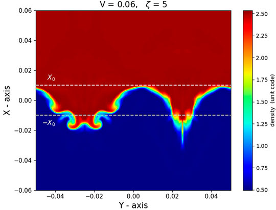
FIGURE 3. Graph shows one snapshot of the region for the Fourier analysis of the v_x(y, z, t) slices.

FIGURE 4

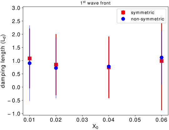
FIGURE 4. Damping length L_d as a dependence of taken width layer X₀. The circle symbol is considered for the symmetric widths, where the square symbol represents the non-symmetric strips.

In the following analysis, we take the averaged power amplitudes of the fundamental mode and follow the peak values with a kink speed (V_k) in the z direction (z_i = V_k t_i) at each time step t_i (Figure 5). The power amplitudes in the fundamental mode values were calculated with the help of $\mathtt{n}\mathtt{u}\mathtt{m}\mathtt{p}\mathtt{y}\mathtt{p}\mathtt{o}\mathtt{l}\mathtt{y}\mathtt{f}\mathtt{i}\mathtt{t}$ package by fitting a parabola to the power to quantify the power in the fundamental mode. The top of the fitted parabola was used further. We can see that the data points decay exponentially (Figure 6). We then fit these data points with the exponential damping profile (exp( − z/L_d)) with damping length (L_d). These damping lengths were used to estimate the damping time with the following expression:

${\tau }_d=L_d/V_k,$

where we have assumed a simple propagating wave.

FIGURE 5

FIGURE 5. The graph shows the power amplitude of the fundamental wave mode as a function of the z axis. The orange curve is the parabolic fit, and the green dots are the approximate peak values of the wave at specific times. Blue dots represent the errors of the $\mathtt{n}\mathtt{u}\mathtt{m}\mathtt{p}\mathtt{y}\mathtt{p}\mathtt{o}\mathtt{l}\mathtt{y}\mathtt{f}\mathtt{i}\mathtt{t}$ function.

FIGURE 6

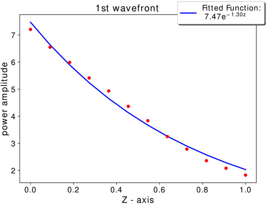
FIGURE 6. The graph illustrates the power amplitude of the fundamental wave mode as a function of the z axis, for the main simulation (V = 0.06, ζ = 5). Red dots represent the followed peak values of the mode at each time step. The blue line is the fitted exponential function (exp( − z/L_d)).

In order to understand the evolution of the wavefront (how it decays and evolves to higher wavenumbers), we need to follow the wavefront as it propagates. If we consider the evolution in terms of time dependence, we can see that there will be a series of waves passing. However, the next wavefront has a similar evolution stage as the first one, except for a slight change in the density structure. This is because it has been smoothed by the mixing of density by the first wavefront. Because of the modification of the wave, we find that turbulence is affected only in a minor way, and there will be a third-order effect on the wave. Therefore, we can conclude that time variation will be third order, and hence the effect of time will be insignificant. Thus, following the wave propagation along the z axis is the crucial point of studying the energy loss.

Figure 7 shows the comparison of our theoretical model with the damping lengths from the simulation for each density contrast and velocity amplitude. The green line represents the theoretical model for the damping time scale Eq. 27. Red squares are the calculated damping time from the simulation for the first wavefront. In comparison, blue dots show the average damping time for the first five wavefronts. The error bars were calculated starting from the Fourier transform by taking the standard deviation σ, where we computed it using $\mathtt{n}\mathtt{u}\mathtt{m}\mathtt{p}\mathtt{y}\mathtt{s}\mathtt{t}\mathtt{d}$ routine. We apply uncertainties on the polyfit function, and the estimated damping length was taken from the fitted exponential function, including the uncertainties from the covariance matrix. The errors on the blue dots are bigger than the red squares due to the loss of the parabolic shape for subsequent wavefronts. Finally, we use the following equation to find the mean and the error in the damping length when averaging over multiple wavefronts as in the paper by Van Doorsselaere et al. (2007).

${\bar{L}}_d=\frac{{\sum }_{i=0}^{N-1}{L}_{d_i}/{\sigma }_i^2}{{\sum }_{i=0}^{N-1}1/{\sigma }_i^2},(29)$

where mean error calculated with

${\sigma }_{{\bar{L}}_d}^2=\frac{1}{{\sum }_{i=0}^{N-1}1/{\sigma }_i^2}.(30)$

We run the simulation with a different driver

$v_x(y,t)=V\cos (\omega t)\sin (k_{y}y)\left\{\begin{array}{c}\exp (\kappa x)\text{if}x\le 0,\hfill \\ \exp (-\kappa x)\text{if}x>0.\hfill \end{array}\right.$

where we take κ = k_y = 2 π/0.1 and V = 0.12, corresponding to the surface Alfvén wave’s analytical eigenfunction. One of the main reasons was to check if the different driver has an effect on the results. Figure 8 demonstrates the results for the simulation by the various drivers adopting the appropriate theoretical solution of the surface Alfvén wave. The z − = 0.3 and t = 3 are applied to the snapshot. We can see the non-linear deformation of the interface different than the initial simulation, but the calculated damping time matches with the theoretical solution.

FIGURE 7

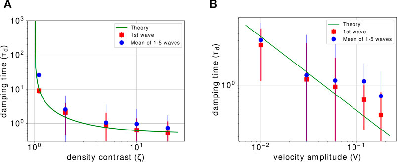
FIGURE 7. Damping time for the propagating wave as a function of density contrast (A) and velocity amplitude (B). The green line represents the theoretical model for the damping time Eq. 27. Red squares are the calculated damping time for the first wave front. Blue dots are the average of the first 5 waves fronts.

FIGURE 8

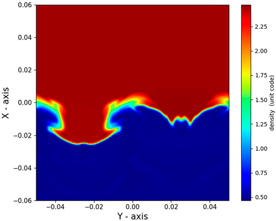
FIGURE 8. The plot shows the simulation result for the different driver taking the relevant theoretical eigenfunction of the surface Alfvén wave. The snapshot is taken at z = 0.3 and t = 3.

We have also simulated with a smaller wavelength k_y, where we take the new wavenumber as $k_y^{\ast }=2k_y$ and compare with Eq. 27. The predicted damping time for the half-wavelength in Eq. 27 gives τ_d = 0.38. The numerically estimated value for the simulation is τ_d = 0.55 ± 0.16. We believe that the discrepancy is that the nonlinear deformation is much faster and might require higher resolution. Moreover, in $k_y^{\ast }$ case, the first wavefront deform faster, loses its parabolic shape faster, and will have it in a shorter period than the k_y.

Lastly, we compare the wavelength of the Alfvén waves in the non-uniform regions and Surface Alfvén waves at the interface. It is known that the phase speed of surface Alfvén waves lies between $V_{Ar}^2$ and $V_{Al}^2$ (e.g., Roberts, 1981; Goossens et al., 2012). The purpose here is to highlight the distinction between classic Alfvén waves and surface Alfvén waves. Obviously,

$\frac{V_{Ar}^2}{v_k^2}<1<\frac{V_{Al}^2}{v_k^2},{\lambda }_{A{W}_r}<{\lambda }_{SAW}<{\lambda }_{A{W}_l}.$

It can easily be seen from the following expression that the Alfvén waves have a shorter wavelength in the upper half than surface Alfvén waves of the non-uniform region. Similarly, they have a longer wavelength in the lower half, which is also confirmed in the numerical simulation (Figure 9). This shows that the uniform driver excites both the surface Alfvén wave and classic Alfvén waves in the top and bottom of the domain. Moreover, the classic Alfvén waves show less damping because they do not have the uniturbulent cascade.

FIGURE 9

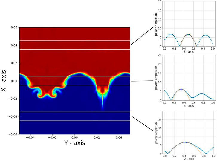
FIGURE 9. Comparison of wave’s amplitude in the fundamental mode for the different regions. It shows that Alfvén waves have shorter wavelength in the upper half, compared to the surface Alfvén waves. Similarly, the lower half has a longer wavelength.

5 Discussion and Conclusion

This study supports the view that plasma inhomogeneity leads to the formation of uniturbulence for propagating kink waves (Magyar et al., 2019b). We performed analytical calculations in incompressible MHD for a 1-D planar equilibrium model with piece-wise constant density. We obtained analytical expressions for the wave energy density, the energy dissipation rate, and the energy cascade damping time. Subsequently, we derived an analytical model to predict the damping time for uniturbulence evolution in surface Alfvén waves. Equation 27 reveals that the damping time is inversely proportional to the perpendicular wave number and the amplitude of the surface Alfvén waves. Significantly, the damping time obtained here corroborates the Van Doorsselaere et al. (2020a) findings for cylindrical configurations. Given that the only difference with that work is the cylindrical vs planar geometry, our numerical study lends additional credibility to the analytical results of Van Doorsselaere et al. (2020a).

We calculated the numerical energy dissipation rate through numerical simulations by performing Fourier transform. We took the fundamental mode of a perpendicular wavenumber (k_y) and estimated the damping time. Specifically, the calculated damping time for A = 0.06 and ζ = 5 case in Eq. 27 gives τ_d = 0.75. Accordingly, the estimated value for numerical simulation is equal to τ_d = 0.85 ± 0.32. Likewise, we compared our theoretical model with a series of 3D ideal MHD simulations, where the similarity is notable (see Figure 7). In particular, numerical results showed that the damping time confirms the inverse proportionality to the density contrast and the amplitude of surface Alfvén waves.

These findings extend our understanding of the role of uniturbulent damping of surface Alfvén waves. We do not imply that our model accurately represents coronal conditions. We have chosen parameters in our simulations to verify the analytically derived energy cascade rate, checking the basic physical assumptions. We have proven that the simulations confirm the analytical equations and that there is an additional energy cascade. Thus, the cascade of surface Alfven waves might play a role in heating the corona. We do not have coronal conditions, but we believe what we simulated also represents how surface Alfven waves would behave in the corona. It is well known that in the solar corona and the solar wind plasmas are structured across the magnetic field (Raymond et al., 2014), where uniturbulence could probably be relevant. Especially in open magnetic field regions, the uniturbulence could provide an additional channel for turbulent cascade and therefore increased dissipation. Uniturbulence could also be applicable in closed magnetic environments, as coronal loops, considering the coherent nature of the interaction. More research is needed in order to verify the significance of this damping mechanism.

Data Availability Statement

The raw data supporting the conclusions of this article will be made available by the authors, without undue reservation.

Author Contributions

RI did analytical calculations, simulations and wrote the initial draft. TV gave feedback on the manuscript and overseeing of research progress. MG gave input on the analytical model. NM gave input on the numerical model. All authors provided critical feedback and helped shape the research, analysis and manuscript.

Funding

This work is supported by the European Research Council (ERC) under the European Union’s Horizon 2020 research and innovation programme (grant agreement No 724326).

Conflict of Interest

The authors declare that the research was conducted in the absence of any commercial or financial relationships that could be construed as a potential conflict of interest.

Publisher’s Note

All claims expressed in this article are solely those of the authors and do not necessarily represent those of their affiliated organizations, or those of the publisher, the editors and the reviewers. Any product that may be evaluated in this article, or claim that may be made by its manufacturer, is not guaranteed or endorsed by the publisher.

References

Anfinogentov, S. A., Nakariakov, V. M., and Nisticò, G. (2015). Decayless Low-Amplitude Kink Oscillations: a Common Phenomenon in the Solar corona? Astron. Astrophysics 583, A136. doi:10.1051/0004-6361/201526195

CrossRef Full Text | Google Scholar

Antolin, P., De Moortel, I., Van Doorsselaere, T., and Yokoyama, T. (2016). Modeling Observed Decay-Less Oscillations as Resonantly Enhanced Kelvin-Helmholtz Vortices from Transverse Mhd Waves and Their Seismological Application. ApJ 830, L22. doi:10.3847/2041-8205/830/2/L22

CrossRef Full Text | Google Scholar

Antolin, P., and Van Doorsselaere, T. (2019). Influence of Resonant Absorption on the Generation of the Kelvin-Helmholtz Instability. Front. Phys. 7, 85. doi:10.3389/fphy.2019.00085

CrossRef Full Text | Google Scholar

Biskamp, D. (2003). Magnetohydrodynamic Turbulence. Cambridge, UK: Cambridge University Press.

Google Scholar

Bruno, R., and Carbone, V. (2005). The Solar Wind as a Turbulence Laboratory. Living Rev. Solar Phys. 2, 4. doi:10.12942/lrsp-2005-4

CrossRef Full Text | Google Scholar

Cranmer, S. R., van Ballegooijen, A. A., and Edgar, R. J. (2007). Self‐consistent Coronal Heating and Solar Wind Acceleration from Anisotropic Magnetohydrodynamic Turbulence. Astrophys J. Suppl. S 171, 520–551. doi:10.1086/518001

CrossRef Full Text | Google Scholar

De Pontieu, B., McIntosh, S. W., Carlsson, M., Hansteen, V. H., Tarbell, T. D., Schrijver, C. J., et al. (2007). Chromospheric Alfvénic Waves Strong Enough to Power the Solar Wind. Science 318, 1574–1577. doi:10.1126/science.1151747

PubMed Abstract | CrossRef Full Text | Google Scholar

Goldstein, M. L., Roberts, D. A., and Matthaeus, W. H. (1995). Magnetohydrodynamic Turbulence in the Solar Wind. Annu. Rev. Astron. Astrophys. 33, 283–325. doi:10.1146/annurev.aa.33.090195.001435

CrossRef Full Text | Google Scholar

Goossens, M., Andries, J., Soler, R., Van Doorsselaere, T., Arregui, I., and Terradas, J. (2012). Surface Alfvén Waves in Solar Flux Tubes. Astrophysical J. 753, 111. doi:10.1088/0004-637X/753/2/111

CrossRef Full Text | Google Scholar

Goossens, M., Hollweg, J. V., and Sakurai, T. (1992). Resonant Behaviour of MHD Waves on Magnetic Flux Tubes. Sol. Phys. 138, 233–255. doi:10.1007/BF00151914

CrossRef Full Text | Google Scholar

Heinemann, M., and Olbert, S. (1980). Non-WKB Alfvén Waves in the Solar Wind. J. Geophys. Res. 85, 1311–1327. doi:10.1029/JA085iA03p01311

CrossRef Full Text | Google Scholar

Heyvaerts, J., and Priest, E. R. (1983). Coronal Heating by Phase-Mixed Shear Alfven Waves. Astron. Astrophysics 117, 220.

Google Scholar

Hollweg, J. V., and Yang, G. (1988). Resonance Absorption of Compressible Magnetohydrodynamic Waves at Thin “Surfaces”. J. Geophys. Res. 93, 5423–5436. doi:10.1029/JA093iA06p05423

CrossRef Full Text | Google Scholar

Ionson, J. A. (1978). Resonant Absorption of Alfvenic Surface Waves and the Heating of Solar Coronal Loops. ApJ 226, 650–673. doi:10.1086/156648

CrossRef Full Text | Google Scholar

Iroshnikov, P. S. (1964). Turbulence of a Conducting Fluid in a strong Magnetic Field. Soviet Astron. 7, 566.

Google Scholar

Keppens, R., Meliani, Z., van Marle, A. J., Delmont, P., Vlasis, A., and van der Holst, B. (2012). Parallel, Grid-Adaptive Approaches for Relativistic Hydro and Magnetohydrodynamics. J. Comput. Phys. 231, 718–744. doi:10.1016/j.jcp.2011.01.020

CrossRef Full Text | Google Scholar

Kohutova, P., Verwichte, E., and Froment, C. (2020). First Direct Observation of a Torsional Alfvén Oscillation at Coronal Heights. Astron. Astrophysics 633, L6. doi:10.1051/0004-6361/201937144

CrossRef Full Text | Google Scholar

Kolmogorov, A. (1941). The Local Structure of Turbulence in Incompressible Viscous Fluid for Very Large Reynolds’ Numbers. Akademiia Nauk SSSR Doklady 30, 301–305.

Google Scholar

Kraichnan, R. H. (1965). Inertial-Range Spectrum of Hydromagnetic Turbulence. Phys. Fluids 8, 1385. doi:10.1063/1.1761412

CrossRef Full Text | Google Scholar

Magyar, N., Doorsselaere, T. V., and Goossens, M. (2017). Generalized Phase Mixing: Turbulence-like Behaviour from Unidirectionally Propagating MHD Waves. Sci. Rep. 7, 14820. doi:10.1038/s41598-017-13660-1

PubMed Abstract | CrossRef Full Text | Google Scholar

Magyar, N., Van Doorsselaere, T., and Goossens, M. (2019a). The Nature of Elsässer Variables in Compressible MHD. Astrophysical J. 873, 56. doi:10.3847/1538-4357/ab04a7

CrossRef Full Text | Google Scholar

Magyar, N., Van Doorsselaere, T., and Goossens, M. (2019b). Understanding Uniturbulence: Self-cascade of MHD Waves in the Presence of Inhomogeneities. Astrophysical J. 882, 50. doi:10.3847/1538-4357/ab357c

CrossRef Full Text | Google Scholar

Matthaeus, W. H., Qin, G., Bieber, J. W., and Zank, G. P. (2003). Nonlinear Collisionless Perpendicular Diffusion of Charged Particles. Astrophysical J. 590, L53–L56. doi:10.1086/376613

CrossRef Full Text | Google Scholar

Matthaeus, W. H., Zank, G. P., Oughton, S., Mullan, D. J., and Dmitruk, P. (1999). Coronal Heating by Magnetohydrodynamic Turbulence Driven by Reflected Low-Frequency Waves. Astrophysical J. Lett. 523, L93–L96. doi:10.1086/312259

CrossRef Full Text | Google Scholar

Morton, R. J., Tiwari, A. K., Van Doorsselaere, T., and McLaughlin, J. A. (2021). Weak Damping of Propagating MHD Kink Waves in the Quiescent corona. APJ 923 (2), 225. doi:10.3847/1538-4357/ac324d

CrossRef Full Text | Google Scholar

Nechaeva, A., Zimovets, I. V., Nakariakov, V. M., and Goddard, C. R. (2019). Catalog of Decaying Kink Oscillations of Coronal Loops in the 24th Solar Cycle. ApJS 241, 31. doi:10.3847/1538-4365/ab0e86

CrossRef Full Text | Google Scholar

Perez, J. C., and Chandran, B. D. G. (2013). Direct Numerical Simulations of Reflection-Driven, Reduced Magnetohydrodynamic Turbulence from the Sun to the Alfvén Critical Point. Astrophysical J. 776, 124. doi:10.1088/0004-637X/776/2/124

CrossRef Full Text | Google Scholar

Popescu Braileanu, B., Lukin, V. S., Khomenko, E., and de Vicente, Á. (2021). Two-fluid Simulations of Rayleigh-Taylor Instability in a Magnetized Solar Prominence Thread. Astron. Astrophysics 646, A93. doi:10.1051/0004-6361/202039053

CrossRef Full Text | Google Scholar

Rappazzo, A. F., Velli, M., Einaudi, G., and Dahlburg, R. B. (2008). Nonlinear Dynamics of the Parker Scenario for Coronal Heating. Astrophysical J. 677, 1348–1366. doi:10.1086/528786

CrossRef Full Text | Google Scholar

Raymond, J. C., McCauley, P. I., Cranmer, S. R., and Downs, C. (2014). The Solar Corona as Probed by Comet Lovejoy (C/2011 W3). Astrophysical J. 788, 152. doi:10.1088/0004-637X/788/2/152

CrossRef Full Text | Google Scholar

Roberts, B. (1981). Wave Propagation in a Magnetically Structured Atmosphere. Sol. Phys. 69, 27–38. doi:10.1007/BF00151253

CrossRef Full Text | Google Scholar

Ruderman, M. S., and Roberts, B. (2002). The Damping of Coronal Loop Oscillations. Astrophysical J. 577, 475–486. doi:10.1086/342130

CrossRef Full Text | Google Scholar

Sedláček, Z. (1971). Electrostatic Oscillations in Cold Inhomogeneous Plasma I. Differential Equation Approach. J. Plasma Phys. 5, 239–263. doi:10.1017/S0022377800005754

CrossRef Full Text | Google Scholar

Shoda, M., and Yokoyama, T. (2018). Anisotropic Magnetohydrodynamic Turbulence Driven by Parametric Decay Instability: The Onset of Phase Mixing and Alfvén Wave Turbulence. Astrophysical J. Lett. 859, L17. doi:10.3847/2041-8213/aac50c

CrossRef Full Text | Google Scholar

Suzuki, T. K., and Inutsuka, S.-i. (2005). Making the Corona and the Fast Solar Wind: A Self-Consistent Simulation for the Low-Frequency Alfvén Waves from the Photosphere to 0.3 AU. ApJ 632, L49–L52. doi:10.1086/497536

CrossRef Full Text | Google Scholar

Terradas, J., Andries, J., Goossens, M., Arregui, I., Oliver, R., and Ballester, J. L. (2008). Nonlinear Instability of Kink Oscillations Due to Shear Motions. ApJ 687, L115–L118. doi:10.1086/593203

CrossRef Full Text | Google Scholar

Thurgood, J. O., Morton, R. J., and McLaughlin, J. A. (2014). First Direct Measurements of Transverse Waves in Solar Polar Plumes Using Sdo /Aia. Astrophysical J. Lett. 790, L2. doi:10.1088/2041-8205/790/1/L2

CrossRef Full Text | Google Scholar

Tomczyk, S., McIntosh, S. W., Keil, S. L., Judge, P. G., Schad, T., Seeley, D. H., et al. (2007). Alfvén Waves in the Solar Corona. Science 317, 1192–1196. doi:10.1126/science.1143304

PubMed Abstract | CrossRef Full Text | Google Scholar

Tu, C.-Y., and Marsch, E. (1995). Mhd Structures, Waves and Turbulence in the Solar Wind: Observations and Theories. Space Sci. Rev. 73, 1–210. doi:10.1007/BF00748891

CrossRef Full Text | Google Scholar

van Ballegooijen, A. A., Asgari-Targhi, M., Cranmer, S. R., and DeLuca, E. E. (2011). Heating of the Solar Chromosphere and Corona by Alfvén Wave Turbulence. ApJ 736, 3. doi:10.1088/0004-637X/736/1/3

CrossRef Full Text | Google Scholar

Van Doorsselaere, T., Goossens, M., Magyar, N., Ruderman, M. S., and Ismayilli, R. (2021). Nonlinear Damping of Standing Kink Waves Computed with Elsässer Variables. ApJ 910 (1), 58. doi:10.3847/1538-4357/abe630

CrossRef Full Text | Google Scholar

Van Doorsselaere, T., Li, B., Goossens, M., Hnat, B., and Magyar, N. (2020a). Wave Pressure and Energy Cascade Rate of Kink Waves Computed with Elsässer Variables. Astrophysical J. 899, 100. doi:10.3847/1538-4357/aba0b8

CrossRef Full Text | Google Scholar

Van Doorsselaere, T., Nakariakov, V. M., and Verwichte, E. (2007). Coronal Loop Seismology Using Multiple Transverse Loop Oscillation Harmonics. A&A 473, 959–966. doi:10.1051/0004-6361:20077783

CrossRef Full Text | Google Scholar

Van Doorsselaere, T., Srivastava, A. K., Antolin, P., Magyar, N., Vasheghani Farahani, S., Tian, H., et al. (2020b). Coronal Heating by MHD Waves. Space Sci. Rev. 216, 140. doi:10.1007/s11214-020-00770-y

CrossRef Full Text | Google Scholar

Verdini, A., Velli, M., and Buchlin, E. (2009). Turbulence in the Sub-alfvénic Solar Wind Driven by Reflection of Low-Frequency Alfvén Waves. ApJ 700, L39–L42. doi:10.1088/0004-637x/700/1/l39

CrossRef Full Text | Google Scholar

Wentzel, D. G. (1979a). Hydromagnetic Surface Waves on Cylindrical Fluxtubes. Astron. Astrophysics 76, 20–23.

Google Scholar

Wentzel, D. G. (1979b). The Dissipation of Hydromagnetic Surface Waves. ApJ 233, 756–764. doi:10.1086/157437

CrossRef Full Text | Google Scholar

Xia, C., Teunissen, J., Mellah, I. E., Chané, E., and Keppens, R. (2018). MPI-AMRVAC 2.0 for Solar and Astrophysical Applications. ApJS 234, 30. doi:10.3847/1538-4365/aaa6c8

CrossRef Full Text | Google Scholar