 C. R. Chappell
 A. Glocer
 B. L. Giles2
 T. E. Moore
 M. M. Huddleston
 D. L. Gallagher
95% of researchers rate our articles as excellent or good
Learn more about the work of our research integrity team to safeguard the quality of each article we publish.
Find out more
REVIEW article
Front. Astron. Space Sci. , 21 October 2021
Sec. Space Physics
Volume 8 - 2021 | https://doi.org/10.3389/fspas.2021.746283
This article is part of the Research Topic Cold-Ion Populations and Cold-Electron Populations in the Earth’s Magnetosphere and Their Impact on the System View all 18 articles
The solar wind has been seen as the major source of hot magnetospheric plasma since the early 1960’s. More recent theoretical and observational studies have shown that the cold (few eV) polar wind and warmer polar cusp plasma that flow continuously upward from the ionosphere can be a very significant source of ions in the magnetosphere and can become accelerated to the energies characteristic of the plasma sheet, ring current, and warm plasma cloak. Previous studies have also shown the presence of solar wind ions in these magnetospheric regions. These studies are based principally on proxy measurements of the ratios of He++/H+ and the high charge states of O+/H+. The resultant admixture of ionospheric ions and solar wind ions that results has been difficult to quantify, since the dominant H+ ions originating in the ionosphere and solar wind are indistinguishable. The ionospheric ions are already inside the magnetosphere and are filling it from the inside out with direct access from the ionosphere to the center of the magnetotail. The solar wind ions on the other hand must gain access through the outer boundaries of the magnetosphere, filling the magnetosphere from the outside in. These solar wind particles must then diffuse or drift from the flanks of the magnetosphere to the near-midnight reconnection region of the tail which takes more time to reach (hours) than the continuously large outflowing ionospheric polar wind (10’s of min). In this paper we examine the magnetospheric filling using the trajectories of the different ion sources to unravel the intermixing process rather than trying to interpret only the proxy ratios. We compare the timing of the access of the ionospheric and solar wind sources and we use new merged ionosphere-magnetosphere multi-fluid MHD modeling to separate and compare the ionospheric and solar wind H+ source strengths. The rapid access of the initially cold polar wind and warm polar cusp ions flowing down-tail in the lobes into the mid-plane of the magnetotail, suggests that, coupled with a southward turning of the IMF Bz, these ions can play a key triggering role in the onset of substorms and subsequent large storms.
In this paper we will review how the Earth’s ionosphere populates the different regions of more energetic particles in the magnetosphere and combined with the changing solar wind Bz can drive the dynamics of the magnetosphere. We will begin with a review of the ionospheric role as a source and end with a focus on more recent results which continue to build the case for the ionosphere’s role as a driver of magnetospheric processes.
The magnetospheric community has always thought about the ionosphere as playing a very important role in storms and substorms as a recipient of energy from the magnetosphere and setting up the current systems that are an integral part of storm dynamics. In this paper we will look differently at that understanding and ask the question, not just how does the ionosphere respond to magnetospheric storms, but how does the ionosphere participate as a driver that causes magnetospheric substorms and storms to happen.
In terms of specific objectives of this paper we will talk about the influence of the ionospheric plasma throughout the magnetosphere, that is in regions like the plasmasphere, plasma trough, polar cap, magnetotail lobes, plasma sheet, warm plasma cloak, ring current, and radiation belts—all of the major areas in which the ionosphere is playing a role.
Initially, we want to show how the ionospheric plasma that has energies of only a few eV can become energized in the magnetosphere to the energies of the different regions in which it ends up and can actually create these regions. We want to look at individual ion trajectories that show how the cold ions are energized in the different regions into which they move. Then in combination with the solar wind Bz, we show how the ionospheric particles can become a major driving mechanism for substorms and storms.
It is also important to call attention to the role of ionospheric plasma in magnetic reconnection and the continuing challenge of measuring low energy plasma. Both the dayside solar wind-magnetosphere and nightside magnetotail reconnection regions become populated with ionospheric plasma. The ionospheric ions, both from the duskside plumes and detached regions that come off the plasmasphere and the warm plasma cloak bring particles to the nose of the magnetosphere and affect the reconnection process there (Fuselier et al., 2019), while high latitude outflow of the polar wind and polar cusp affects magnetotail reconnection (Toledo-Redondo et al., 2021). These initially polar wind ions are very difficult to measure in the lobes because of their low energies and densities and the effects of positive spacecraft potential, which means that they are often unseen. Most of our early measurements of the magnetosphere had no observations of any particles in the lobes of the tail. In addition, the ambient low energy electrons were almost impossible to measure amidst the spacecraft charging and the photoelectrons that are created by the action of the sunlight on the different materials on the spacecraft surfaces.
Figure 1 is a decades old sketch of the magnetosphere that was originally created to show the solar wind entry (pink regions at the sunward boundary) into the magnetosphere and formation of the distinctive regions of the magnetosphere. This figure originally was missing two very important things. We did not know about the polar wind at that time, the very low-energy few eV outflowing H+ and He+ ions, and we could not tell the difference between H+ ions that came from the solar wind and H+ ions that came from the ionosphere. To the measurements that we are able to make, these two sources of H+ look exactly the same. To distinguish between the two, we will have to model that difference with multi-fluid merged ionosphere/magnetosphere MHD models which will be discussed later in this paper.
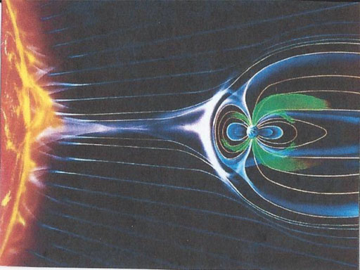
FIGURE 1. A sketch of the solar-terrestrial connection that includes the contribution of the Earth’s ionosphere to the magnetosphere.
Those two things, the inability to see the outflowing polar wind, which had not been even theoretically predicted until 1968 (Banks and Holzer, 1968, Banks et al., 1971) and the inability to tell the difference between solar wind and ionospheric H+, gave us the misimpression that all of the magnetospheric plasmas with the exception of the plasmasphere (the blue region close to the Earth in Figure 1) came from the solar wind. After the theory and measurements of the 1970’s, 80’s, and 90’s (Hoffman, 1970; Nagai et al., 1984; Chandler et al., 1991; Abe et al., 1996; Moore et al., 1997; Yau and Andre, 1997), the green outflowing ions were added to this conceptual image of the magnetosphere.
Our early measurements in the late 50’s and early 60’s also led us to the same inaccurate “solar wind only” conclusion because early on in space missions, we could only measure the very high energy particles but not the low energy ones. Geiger counters were flown on the early explorer satellites and measured the radiation belts (MeV). Then with the development of channel electron multipliers, experimenters were able to measure ion and electron energies down to ∼100 eV in particle detectors and we started seeing the plasma sheet and the ring current. Some of the early spaceborne ion traps and ground-based whistler observations could measure the higher densities (>10 ions/cm3) of the plasmasphere down to a few eV (Carpenter, 1963; Gringauz, 1963), but the spacecraft, particularly those which went farther out into the magnetosphere that had no spacecraft potential control, could not see the low energy particles with energies less than 10’s of eV.
This combination of factors led researchers to think that the solar wind was delivering most of the particle populations to the magnetosphere, a conclusion which is now being challenged by more recent data. Research at the Lockheed Palo Alto Research Laboratory in the early 1970’s using the Light Ion Mass Spectrometer on the OGO-5 satellite (Harris and Sharp, 1969) gave new information on the low energy, few eV ions in the magnetosphere with a particular emphasis on the dynamics of the plasmasphere. The filling and draining of the plasmasphere and its changes in size and shape were intriguing (Chappell et al., 1970; Chappell, 1972). It was realized that measurements of the low-energy (0–50 eV) ions were needed using instruments that had higher sensitivities and a spinning spacecraft so that pitch angle distributions as well as composition and energy could be determined. These measurements would give an understanding of how the ions were moving and, in particular, how they were flowing upward out of the ionosphere to fill the plasmasphere. In this same time period, satellite measurements had shown the presence of energetic O+ at high altitudes indicating both an ionospheric source and the ability to energize the originally cold ionospheric ions (Shelley et al., 1972).
NASA created the Dynamics Explorer mission and a new group, now at the NASA/Marshall Space Flight Center proposed an instrument, the Retarding Ion Mass Spectrometer, for the mission and was selected (Chappell et al., 1981). Dynamics Explorer was a two polar, co-planar spacecraft mission, one in a low Earth orbit to measure the atmosphere and ionosphere and one with a 4 Re apogee that could see the outflowing ions as they left the ionosphere and entered the magnetosphere. The RIMS instrument was on the higher altitude spacecraft. It was an interesting time in which the members of the science working group for the mission were trying to decide when in the orbit the different instruments would be operated because there wasn’t enough telemetry to run all of them all the time. This led to spirited discussions between the RIMS group, whose interest was to measure at lower to middle latitudes so that the plasmasphere could be studied, and the investigators who wanted to measure the polar cap region to study the aurora.
The investigator group compromise led to RIMS low energy ion measurements in both the low latitudes and the high latitude polar regions. That turned out to be an important decision, because what was observed, when the Dynamics Explorer 1 spacecraft was up over the polar regions, was that there were very large fluxes of ion outflow. It came from the polar wind (Nagai et al., 1984), the polar cusp (Gurgiolo and Burch, 1982), the nightside auroral zone (Yau et al., 1985) and was all seen at high latitudes; this changed our perspective significantly
At this time in the mid-80’s it was realized that there was a lot of ion outflow that was seen from RIMS (Lockwood et al., 1985; Giles et al., 1994) and also from the Lockheed instrument at higher energies, the Energetic Ion Composition Spectrometer, (Shelley et al., 1982; Yau et al., 1985) and a mass spectrometer on the Akebono spacecraft (Yau and Andre, 1997). These large amounts of ions were flowing upward out of the polar cap, the polar cusp and nightside auroral regions. This led to the thought about whether there was enough outflow so that if one estimated where the ions could go back in the magnetotail, it would give the observed densities in these higher altitude regions of the magnetosphere that had already been measured at higher energy (See Figure 2). This was confirmed; there was enough ion outflow from the polar regions that could move up through the lobes of the tail to the mid-plane to make the plasma sheet and the ring current, although back then the low energy lobe ions were invisible to spacecraft flying in the lobes because of the positive spacecraft potentials.
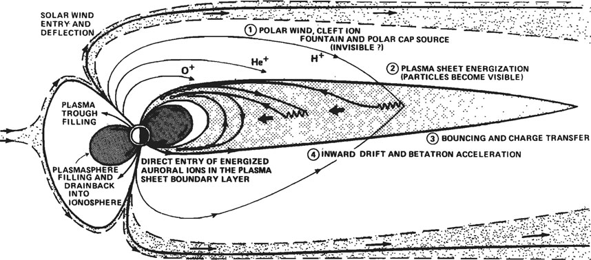
FIGURE 2. A schematic look at the process by which the Earth’s ionosphere might supply plasma to the different regions of the magnetosphere (Chappell et al., 1987).
Although the low energy outflow could not be seen in the lobes, it could be seen by the RIMS instrument down at a few Re altitude (Nagai et al., 1984). RIMS also had an aperture plane around the entrance to the instrument that could be negatively biased to help offset the positive spacecraft potential. But still, all of the spacecraft that operated at higher altitudes in the lobes measured no low energy ions. In the (Chappell et al., 1987) paper it was speculated that the low energy polar wind ions must be invisible in the lobes of the tail because of positive spacecraft potential, but the low altitude data and calculations showed that there was enough of it to create the observed densities of the plasma sheet and the ring current. The DE RIMS measurements started the thinking about the ionosphere as a source of magnetospheric particles.
Subsequent to the Chappell et al., 1987 paper, Dominique Delcourt did ion trajectory modeling (Delcourt et al., 1993) which showed that not only did the outflowing ionospheric ions flow through the lobes into the mid-plane of the magnetospheric tail with enough flux to create the densities that had been measured in the plasma sheet and ring current, but that in addition, these initiatively low energy polar wind and polar cusp outflowing ions would become energized in their trajectories to create the energies that are found in these regions of the tail—enough density and enough energy!
Given that low energy ions can move up out of the ionosphere, across the polar cap into the lobes of the tail and then into the mid-plane of the tail, it is important to think about the magnetosphere in a different way. We tend to think about it in terms of the distinctive plasma populations observed in differing regions with distinguishing energies and behaviors. We think about the lobes, the plasma sheet, the ring current, the warm plasma cloak, the plasmasphere, and the radiation belts. Our thinking about regions of plasma tends to conceptualize the magnetosphere as a superposition of these regions, but there is a growing realization that they are an interconnected continuum, a tapestry, of plasma transport and physical processes. The pictures (regions) on tapestries are made by a series of threads of different colors that are woven into this tapestry to create the images that you see.
As in the tapestry’s threads, the observed regions of the magnetospheric system are created by the motion of ions and electrons flowing through the magnetosphere, while being energized by the cross-tail potential, parallel potentials, wave-particle interactions and reconnection. A single ion can start in the ionosphere as a polar wind ion with an energy of few eV and flow into the polar cap, where it can pick up additional energy and then move into the lobes, making 10–100 eV ions. (Figure 3).
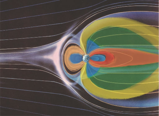
FIGURE 3. A schematic look at the flow of ionospheric plasma from the Earth upward into the magnetosphere to form the different regions of hot plasma.
After it has been a 1 eV and then tens of eV in the polar cap and lobe it can convect into the plasma sheet, by a process that will be discussed later, and can be energized by curvature drift in the cross-tail potential and reconnection to the keV energies that are observed in the plasma sheet. As it drifts back earthward, it can be energized further by the cross-tail potential and betatron acceleration to make the ring current energies (10’s of KeV) in the midnight to dusk sector, which we observe (Huddleston et al., 2005). Some of the outflow that enters the tail closer to the Earth and on the dawnside of the magnetosphere acquires less energy and makes the warm plasma cloak in the midnight to noon dawnside sector (Chappell et al., 2008).
This is the tapestry and the challenge will be to try to measure the motion of all the ions and electrons which create it. Their presence contributes substantially to the environment of the plasma sheet in which reconnection subsequently takes place. It is important, but it is difficult to understand the magnetosphere just from the point of view of moments and composition ratios. Those are valuable; the ratio of H+ to He++ is valuable as a rough indicator of the solar wind source, just as H+, He+ and O+ are indicators of the ionospheric source, but they can be difficult to explain without knowing their trajectory time history.
A corollary perspective emphasized by the tapestry concept and that should be mentioned is that while the level of magnetic activity is an important indicator of what’s going on in the magnetosphere. But the magnetosphere, this magnetic activity from the currents in the ionosphere and the ring current are more a result of what the solar wind and magnetosphere have done than a cause, although we correlate with these indices because they tell us that the magnetosphere is in different states of dynamic change. It is important to keep in mind that these magnetic indices show the results of the magnetospheric dynamics that began earlier in time and are not the cause!
As we think about the role of the ionospheric source in the magnetosphere, there are two types of particles that flow out of the ionosphere and we have named them after the people who largely discovered them. One group is called Strangeway particles. Strangeway particles are based on the papers that Bob Strangeway has written using FAST data (Strangeway et al., 2005). These are particles that require energy input, such as precipitating particles and waves from the magnetosphere, in order to heat the ions and electrons enough that they can escape the gravitational confinement and flow upward out of the ionosphere. That happens typically in the polar cusp and the nightside auroral zone and they can escape into the magnetosphere. These particles do certainly vary with the solar wind conditions and particularly the Bz component of the solar wind interplanetary magnetic field.
The other particles are Banks and Holzer particles that are named after Peter Banks and Tom Holzer whose theoretical work together with Ian Axford (Banks and Holzer, 1968) showed that the top of the ionosphere should be sending off a flow of plasma, referred to as the polar wind, all the time, even with no external energy input, beyond that provided by the sunlight, which creates the F- region of the ionosphere. On the topside of the F-region, there is a charge separation electric field that forms between the dominant O+ ions and the electrons, that can accelerate the minor ions off the top of the ionosphere, H+ and He+ principally. These supersonic light ions can fill up the plasmasphere at low to mid-latitudes, and at higher latitudes, can flow across the polar cap and out into the lobes.
The polar wind ions can be further energized as they flow through the polar cusp, across the polar cap and auroral zones by both waves and precipitating particles as well as centrifugal acceleration becoming a more “generalized” polar wind (Schunk and Sojka, 1997; Barakat and Schunk, 2006). At lower L shells, the upward polar wind fills up the plasmasphere, and at L-shells above, approximately eight on the dayside, the polar wind will flow poleward through the polar cusp and the convection field will carry it across the polar cap and out into the lobes of the magnetotail.
Of these two types of particles, the Strangeway particles which require energy input from above to escape the ionosphere, such as precipitating particle energy and wave energy, can also be accelerated to higher even higher energies. The Banks and Holzer polar wind, which flows off the top of the ionosphere all the time, from any location in which the ionosphere is in the Sun, gives very large upward fluxes and requires no extra energy from external sources. The Banks and Holzer polar wind flux of 90% H+ and 10% He+ which is of the order of 3 x 10⁸ ions/cm2 sec or 1025–1026 ions/sec flowing out of the ionosphere into the lobes and into the magnetosphere, is a substantial contributor of ions and electrons (Andre and Yau, 1997). The Strangeway particles are also substantial contributors, mostly O+, H+, He+, with fluxes as high as 109 ions/cm2sec, but from the auroral oval dominantly. Their total upward flux is more limited because the total ionospheric area from which they flow out is more limited than the large area of sunlit ionosphere from which the polar wind originates.
Figure 4 shows measurements of Strangeway particles in the lobe of the tail. These measurements are from Liao et al. (2010) using mass spectrometer data from the Cluster spacecraft. This is outflowing O+ (Liao et al., 2010; Mouikis et al., 2010; Kistler et al., 2010). The Sun is off to the left in each one of these pictures. This is basically when the Cluster spacecraft was in the lobes out to about 20 Re, sampling ions that were coming out of the polar cusp. The three vertical panels show the dawn-side, center and dusk-side of the tail, and then non-storm time, storm main phase and recovery in the three rows. The colors on the right show the occurrence frequency. One can see that red is 100%, yellow 75%, down to blue around 25% or less. In the center of the tail, there is a very high probability of seeing cusp outflowing particles in the lobes of the tail. Those are the Strangeway particles and they can come out of the night side auroral zone as well. The nightside auroral zone would typically feed upflowing particles directly into the earthward part of the plasma sheet or the conjugate hemisphere rather than through the lobes as is the case with the upflowing ions from the polar cusp.
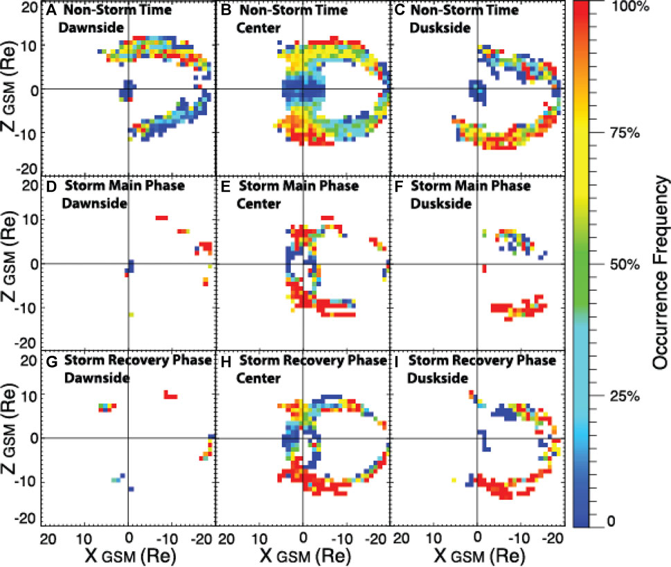
FIGURE 4. Observations from the Cluster satellite of outflowing O+ ions from the polar cusp seen in the lobes of the magnetotail.
Some of those outflowing particles can go through regions like the polar cusp or the night side auroral zone where they get further energized. There is also a basic process that energizes the polar wind continuously (Figure 5). This is an ion trajectory that is from Huddleston et al., 2005 using the modeling developed by Delcourt et al., 1993, and Delcourt et al., 1994, and looking at Polar satellite data from the Thermal Ion Dynamics Experiment, TIDE (Moore et al., 1995) and modeling the ion trajectories. Work on this topic was also done by Horwitz, 1994, and John Cladis (1986, 2000). The figure shows an ion leaving the ionosphere with the Sun to the left.
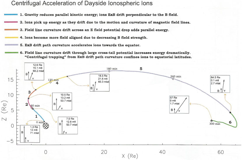
FIGURE 5. The trajectory of a polar wind ion moving from the dayside ionosphere out through the polar cap and tail lobes to the plasma sheet and its energization.
On the dayside, the upflowing particle is the polar wind moving upward at a few eV. It follows the magnetic field lines, and as it moves up into the magnetosphere, it goes through an area where the field line is curved. When it’s curved, it causes a curvature drift on the particle which in this case is out of the page. That drift moves the particle across the cross-tail potential and energizes it. Few eV ions can become 10 eV, and then they flow out through the lobes.
A river of ions continuously flows outward through the magnetospheric lobes as shown by the trajectory. Along the ion trajectory are times; 2 hours, out to about 6 hours by the time it gets to the plasma sheet in the mid-plane of the tail at 60 Re. When it is in the lobes; it is very low energy, 10s of eV, until it reaches the mid-plane of the magnetotail. At that point there can be very distended or stretched magnetic field lines and this creates a very large curvature drift again, out of the page of the figure, and the ion drifts in the direction of the cross-tail potential and gets further energized to keV.
This process will be examined in more detail later in the paper. This figure shows that a few eV polar wind particle can become more energized in the lobe and then further substantially energized as it moves into the mid-plane region. This illustrates that prior to missions like Polar which had high sensitivity low energy ion instruments and spacecraft potential control, we could not see what was happening in the lobes and our ideas about how the magnetosphere fills were shaped without this information. The fact that there was H+ in the solar wind and H+ in the plasma sheet with about the same energies, made it seem natural that the solar wind was the source of the plasma sheet. As it turned out there are large fluxes of low energy plasma continuously flowing through the lobes into the plasma sheet region, as subsequent missions would clearly show (Liemohn et al., 2005).
Figure 6 shows a segment of one orbit of measurements from the POLAR spacecraft TIDE instrument, looking at the low energy ions. The lower panel shows an energy-time spectrogram for 1–400 eV, ions and the upper panel is a spin angle-time spectrogram showing the two magnetic field directions (+ and–symbols) and the ram velocity direction. (x symbol). Knowing that the polar wind ions could not be seen in the lobes unless the spacecraft potential could be controlled, the TIDE investigator group added a plasma source instrument, which sends out an ion-electron xenon plasma so that the spacecraft could draw back the charge that it needed to hold itself at the plasma potential of about one volt (Moore et al., 1995). The photoelectrons leaving the surface of the spacecraft typically charge it positively, so a cloud of electrons and ions can be ejected from the spacecraft enabling the spacecraft to draw back the electrons it needs to neutralize the positive charge.
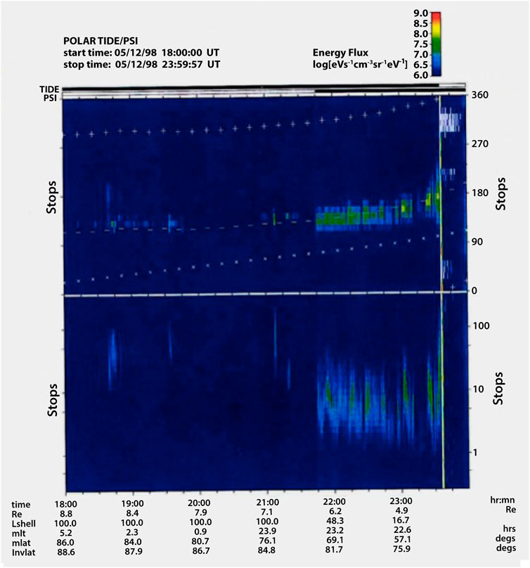
FIGURE 6. A segment of data on the polar wind measured by the TIDE instrument on Polar taken in the lobe of the magnetotail showing the important effect of the plasma neutralizing device.
The solid lines across the top of Figure 6 show when the TIDE instrument (top line) and the PSI spacecraft potential device (second line down) are operating. At the beginning of this panel, the PSI is turned off and we see no ions at low energies in the lower panel. At 2145 UT, the PSI neutralizer is turned on and the low energy polar wind ions appear in the lower panel which is an energy-time spectrogram. The polar wind is seen flowing along that magnetic field line out of the northern hemisphere. We’re looking at polar wind energies here now of 1–10 eV, whereas before the neutralizer turned on, there was nothing to see except a few particles that were up in the 100 eV range. The polar wind is out in the lobes which contain outflowing polar wind as long as the ionosphere location that feeds that flux tube was in the sunlight. This is a very important result! The TIDE instrument on Polar was able to measure the outflowing polar wind at altitudes from just above the ionosphere to its apogee at 9 RE and give the characteristics of the outflowing polar wind (Su et al., 1998). Using these polar wind outflow measurements, the strength of the ionospheric source was also measured, Chappell et al., 2000.
On the Cluster mission there was an ion emitter device to help control spacecraft potential. There was also a very clever complement of instruments that could measure the wake direction of the plasma that was flowing past the spacecraft when the satellite was in the lobe (Engwall et al., 2006; 2009a; 2009b). The investigators could measure the characteristics of the wake, the direction that the ions were flowing, and what their energies and fluxes were. They found out that the lobe contained polar wind ions and electrons (Banks and Holzer particles) as shown in Figure 7 in addition to the polar cusp particles (Strangeway particles) shown in Figure 5.
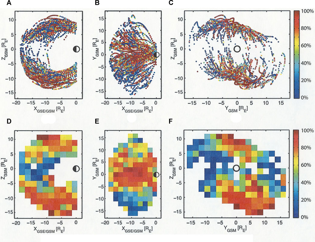
FIGURE 7. Measurements of the polar wind in the lobes of the magnetotail using the spacecraft wake from a group of plasma and field instruments on Cluster.
For the few eV polar wind particles, the fluxes that were measured in the lobe by the Cluster experiment were equal to what had been predicted by the theory almost 20 years before! Figure 7 shows orbital segments of the Cluster spacecraft location in the tail lobes. The scale on the right-hand side is the occurrence frequency of polar wind observations varying from 100% in red all the way down to 0% in blue. The Cluster spacecraft is going through the lobe, then the plasma sheet, then the other lobe. The substantial red, and red-yellow shading shows that along those orbits, the lobe has polar wind flowing out. The left-hand figure is looking from the dawnside of the magnetosphere with the Sun to the right. The middle figure is looking down from above the North Pole and one can see the red part of the orbits are in the center of the tail as expected. The right-hand figure is looking from behind the Earth toward the Sun. The polar wind is seen in the lobes both north and south of the plasma sheet. A suggestion here is that one does not expect to see the polar wind outflows in the plasma sheet region because the polar wind will become energized and have its distribution changed which will not permit this wake technique to work. This also supports the idea that the polar wind/lobal wind flows into the plasma sheet where it is transformed to become an important part of the plasma sheet with different energy and pitch angle characteristics!
The Cluster wake measurements (Engwall et al., 2009b; Andre and Cully, 2012) as well as the direct polar TIDE measurements using the plasma neutralizer show the omnipresence of the polar wind in the lobes (Liemohn et al., 2005). Figure 8 is from Haaland et al., 2012 using data from the Cluster mission looking at where the outflowing polar wind goes, as a function of the southward component of the IMF Bz in the solar wind. When the Bz is southward, the magnetic merging of the solar wind magnetic field with the magnetosphere increases the strength of convection electric field and the cross-tail potential and that causes the outflowing polar wind in the lobes to be pushed into the center part of the tail and energized.
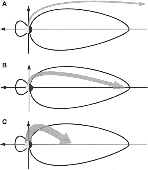
FIGURE 8. The paths of the outflowing polar wind as measured on the Cluster spacecraft showing the influence of the solar wind Bz.
Panel a shows a northward Bz, where there is no convection electric field in the magnetotail. The polar wind comes out of the polar cap and vents out of the tail. Haaland et al., 2012 shows that 90% of the polar wind exhausts out of the back of the tail during northward Bz. A small amount of the exhausting polar wind may get caught up far back down the tail, but during northward positive Bz, it mostly vents out. In panel b, as soon as the solar wind turns Bz southward, there is an increasing cross-tail potential and convection field that starts to drive the polar wind into the plasma sheet region. The higher the southward Bz is, as shown in panel c, the closer to the Earth these ions are convected into the plasma sheet region. Haaland was able to estimate that 90% of the ions that were flowing down the tail and flowing out the back of the tail, in northward Bz conditions, are driven into the plasma sheet during southward Bz conditions and are then able to have a significant influence in creating the plasma sheet environment in which reconnection subsequently takes place. Earlier work by Cully et al., 2003a and Cully et al., 2003b also showed the linkage between outward flowing ions from the ionosphere and their access into the plasma sheet region.
The length of time involved in supplying ionospheric and solar wind plasma to the magnetosphere is a very important element in assessing their relative strength and their impact on the dynamic processes that they drive. The purpose of this section is to develop an idea of how the solar wind plasma versus the ionospheric plasma contributes to the plasma sheet, ring current and warm plasma cloak.
It is possible to do the proxy measurements of He++/H+ and O6+/H+ for the solar wind and O+/H+ or He+/H+ for the ionosphere, but it must be remembered that for the H+ part of these ratios, it is not known where the H+ came from because solar wind H+ looks exactly like ionospheric H+, from a measurement point of view.
Figure 9 shows an ion trajectory starting in the dayside ionosphere as a polar wind ion and moving through the polar cap and lobe into the plasma sheet and subsequently the ring current. This ion trajectory code was developed by Delcourt et al. (1993) and was used by Huddleston et al. (2005) as a way of interpreting the ion characteristics that were being measured by the TIDE instrument on the POLAR spacecraft. The trajectory calculations show how the ion moves from the ionosphere through the magnetosphere, how it changes energy and how long it takes to make this journey. This trajectory model uses a Tsyganenko magnetic field model (Tsyganenko, 1989) and a Weimer convection field model. This case is set up for a Kp of 2. The ion is started on the dayside up above the ionosphere at 10 eV. In additional trajectories that were calculated in this study, the polar wind outflow as measured directly by the Polar TIDE instrument taken near perigee is used as input for the trajectory modeling and the resultant ion trajectory and energization is compared with the same TIDE instrument data taken near apogee.
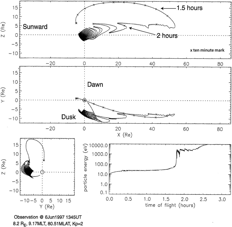
FIGURE 9. An ion trajectory beginning above the ionosphere on the dayside and moving through the lobes and plasma sheet with its subsequent energization.
The timing marks along the trajectory are important. There are 10-min tic marks along the outward trajectory. It shows that from the time the ion leaves the ionosphere, out to the middle of the lobe at 40 RE, takes 90 min, and for the next 20 min, it moves into the plasma sheet region, gets energized, and is moving earthward to become part of the ring current. This top panel views the magnetosphere from the duskside (XZ plane) and traces the motion of an ion that started at 10 eV and ends up with ring current energies. The middle panel looks down on the magnetosphere from the top (XY plane). Here, the ion starts on the dayside, goes over the polar cap into the dusk sector becoming the plasma sheet, and then moves earthward, to become the ring current. The small square panel on the lower left views the ion trajectory from the tail toward the Sun (YZ plane), and the panel on the lower right shows the changing energy of the ion with time. It starts with 10 eV, slightly above polar wind energy, and for that first hour and a half, it increases up to a few 10’s of eV. When it goes into the plasma sheet region at 1.7 h, it gains a kilovolt of energy in about 10 min! That’s, again, from the curvature drift in the cross-tail field that gives it a kilovolt, and then as it drifts earthward, it is further betatron accelerated until it reaches ring current energies of 10 kilovolts.
Now let’s look at the timing. It is about an hour and a half to get from just above the ionosphere on the dayside out to the middle of the lobe at 50 RE. The timing from the lobe into the plasma sheet region is only tens of minutes. If the lobe is full and if the Bz of the solar wind goes southward, these ions are going to move into the plasma sheet within 10–20 min. Later we will come back and look at how long it takes a solar wind particle to get into that region. In this example the same ion which begins as the polar wind, becomes the lobal wind, then the plasma sheet, and finally the ring current. It is the same ion moving through the magnetosphere, and of course, there are a very large number of ions doing this. For the polar wind, there are a few times 1026 ions/sec “threads in the magnetospheric tapestry.”
In looking at the ion trajectory calculation approach, some colleagues have expressed hesitation about just using an isolated ion trajectory because they are concerned that the magnetosphere model is not self-consistent. The model does not let the currents flow and change the magnetic field configuration and strength self-consistently. In this case that is true, however we find that the ion trajectory is an excellent “pathway” to show us how the magnetospheric tapestry is woven. In addition, Alex Glocer has now developed a model that was published just this past year (Glocer et al., 2020) which is a merged ionosphere/magnetosphere, multi-fluid MHD model which has the self-consistent solutions.
The model presented in Glocer et al. (2020) generates the outflowing polar wind from the ionosphere and follows this plasma as it transverses the magnetosphere. It includes a plasmasphere, a ring current, a plasma sheet, and the model is multi-fluid. The model is able to use separate fluids for the ionospheric H+ and the solar wind H+ and thus tell us where these H+ ions originate. This model can tell the difference in where these H+ ions came from. Since H+ is the dominant ion, the ability to separately track the ionospheric and solar wind H+ ions gives unique and very important new results. We will look at his model in more detail later in the paper.
Figure 10 from Glocer et al. (2020), addresses the concern about the utility of using single ion trajectories. This is the trajectory of an ion in the Glocer merged model in a situation similar to the Huddleston ion trajectory. The Sun is to the right in this figure. The color chart shows the ion thermal energy as it moves through the modeled trajectory. The ion flows out of the ionosphere at about 10 eV and then through the polar cap and lobe. By the time it gets across the polar cap and through the lobe and approaches the plasma sheet region it has about 100 eV of energy. Then note that the color of the trajectory changes to yellow, showing that the ion very quickly is energized to 1 keV, and then as it flows back in toward the earth, the color changes to red; it is 10 keV. The results of polar wind, lobal wind, plasma sheet and ring current is what the full merged ionosphere/magnetosphere MHD treatment is showing and it is conceptually very similar to the trajectory and energization given in the Huddleston et al., 2005 results. Although the fluid and particle pictures are conceptually similar, it is important to keep in mind that numerical resistivity drives heating near the x-line in the MHD simulation.
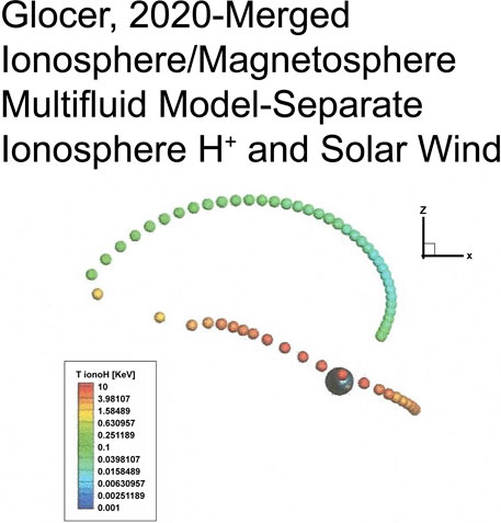
FIGURE 10. An ion trajectory beginning above the dayside ionosphere and its movement through the polar cap and lobe to become energized upon entry into the plasma sheet and ring current (Glocer et al., 2020).
Now, in contrast to the ionospheric source timing of lobe/plasma sheet access and energization to 1 KeV in 20 min, we examine the solar wind source timing. Figure 11 shows recent calculations regarding solar wind access to the magnetosphere by Sorathia et al. (2019). This paper looks at trajectory modeling of solar wind particle access during changing solar Bz. This paper calculates the trajectories of ions that start at the bow shock and then flow into the magnetosphere and the model results show where the solar wind particles go and how long it takes. This is with a northward Bz.
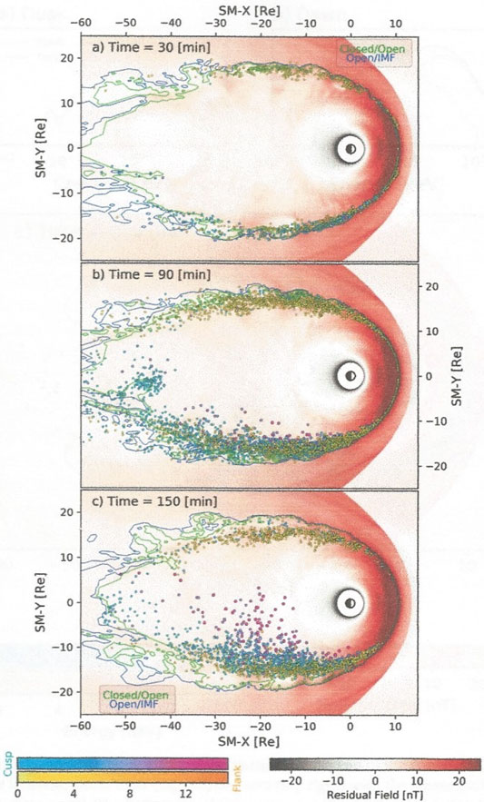
FIGURE 11. A model (Sorathia et al., 2019) showing the flow and timing of solar wind H+ from the bow shock to the flanks of the magnetotail with subsequent diffusion toward the center of the tail.
One of the things that is mentioned in the Sorathia et al., 2019 paper is that it is in northward Bz times in the solar wind that one expects Kelvin-Helmholtz instabilities to be stronger, giving more solar wind access through the flanks into the plasma sheet. This modeling also has reconnection included, but of course, with a northward Bz, it’s not full reconnection but partial just because of the magnetic field orientation in the solar wind.
The timing for access is shown in Figure 11. Panel a shows that for a particle to get from the bow shock to the flanks of the plasma sheet, not into it, but out on the flanks, takes 30 min. In Panel b it is an hour and a half before the solar wind ions begin to have penetration into the plasma sheet from the flanks. These are solar wind H+ ions. In Panel c we see that it takes two and a half hours before these H+ solar wind ions that started out at the bow shock begin to reach toward the center of the plasma sheet in the 20 to 30 RE region. In contrast, the ionospheric ions that are flowing out through the lobes, because they are already in the center of the lobe and are very close, can get into the plasma sheet in 10–20 min. For ions that come from the solar wind, it can take 2 hours or more to reach the reconnection region at the center of the plasma sheet even starting at the flanks. The ionosphere is in a very favorable position to supply plasma to the center of the tail because it has started inside the magnetosphere and because its continuous outflow is already in close proximity to the midnight sector of central plasma sheet just outside in the lobes.
Modeling of the Earth’s magnetosphere has been carried out over the years leading to important advances in our understanding of magnetospheric dynamics (Fok, 1999, Winglee, 2000, Moore et al., 2005, Glocer et al., 2009, Welling and Ridley, 2010, Brambles et al., 2010, Welling et al., 2011, Welling and Ridley, 2010. Recent multi-fluid models have brought an enhanced capability in understanding the role of different sources of plasma for the magnetosphere.
Figure 12 shows the Glocer et al. (2020) results for a case study which uses the merged ionosphere/magnetosphere multi-fluid MHD model that separates the ionospheric H+ from the solar wind H+. It also shows that outflow from different hemispheres makes an important difference. Both lobes aren’t filled symmetrically, but there exists a strong seasonal effect associated with what portion of the ionosphere is illuminated. The solar zenith angle is an important element of the ion/electron production in the ionosphere.

FIGURE 12. Results of a merged multi-fluid model of a storm period showing the relative contributions of the ionosphere and solar wind to the magnetosphere.
Figure 12 from Glocer et al. (2020) shows three sets of four smaller panels which we summarize in the following discussion. The top set is in the main phase of a June 2013 storm as shown by the Dst small panel (lower right) of the larger panel and the location of the vertical line in this panel. The second set of panels is in the storm peak and the third set panels shows the early recovery phase. Within each large panel the upper right panel shows the ionospheric H+ outflow (polar wind), the upper left panel shows the ionospheric O+ outflow (polar cusp) and the lower left is the solar wind H+ component. This case gives us an indication of the relative contribution of the ionospheric plasma as compared to the solar wind in the magnetosphere. The color bar on the right of each plot shows the % contribution. The yellow indicates that 100% of that area is filled by the species on that plot and blue indicates no contribution by that species in that area of the plot. The model has been run for an approximately 24 h period for this isolated storm.
In the top panel set of Figure 12 the main phase, there is a relatively higher proportion of ionospheric H+ (upper right) in the southern hemisphere; there is more in this lobe because it’s favorably positioned with respect to solar illumination. There is ionospheric H+ outflow coming out of both hemispheres, but it is dominant up to 100% in the southern lobe and is from the ionosphere. The upper left plot is the ionospheric O+ outflow from the polar cusp and some from the auroral zone. The cusp is making about 50% of the outflow in the northern lobe. The solar wind presence is dominantly outside the magnetosphere with some penetration on the dayside with the plasma sheet region and lobes showing very little solar wind H+ inside about 30 RE with the southern lobe and plasma sheet being dominated by the outflowing ionospheric H+.
The middle panel set shows the storm peak. At this time in the Glocer et al. (2020), study the ionospheric H+ and O+ fill more of the lobes and plasma sheet volumes with less H+ from the solar wind in these regions. This model also includes the presence of the plasmasphere which results in the calculated cross-tail potential being smaller in magnitude than the simulation without the plasmasphere. The presence of the plasmasphere model appears to have an important influence on the polar cap potential and the Dst in the simulation. Note that the southern lobe of the magnetosphere continues to be dominated by the ionospheric H+ throughout the storm as would be expected for the seasonal effect. The outflowing O+ from the northern polar cusp also continues to dominate that hemisphere as well as the plasma sheet and ring current.
There is very little solar wind H+ in the plasma sheet and ring current regions out to the 20–30 RE equatorial region of the plasma sheet throughout this particular storm. At the storm peak, the solar wind H+ is a very minor component in the equatorial plasma sheet out to 40 RE.
The bottom panel set shows the early recovery phase of the storm, where there is solar wind H+ penetration filling into the down tail regions of the plasma sheet at 30–40 RE and displacing some of the ionospheric plasma prior dominance. The polar wind is still flowing out as seen in the upper right small panel, but it is starting to vent out the tail. The O+ in the upper small panel is still there but diminishing, and the solar wind H+ is beginning to penetrate. The Glocer et al. (2020) model shows that in the peak of this storm, the ring current content is dominated by the H+ from the ionosphere plus O+ from the ionosphere with some minor contribution in the ring current of the H+ that comes from the solar wind.
In order to show the relative contributions of the ionosphere versus the solar wind more clearly, we have added the ionospheric polar wind H+ outflow together with the ionospheric polar cusp O+ outflow and compared this total ionospheric contribution with the solar wind H+ contribution. Figure 13 shows the three times indicating the main phase, storm peak phase and early recovery phase from this selected storm with the total ionospheric H+ and O+ shown in shades of blue and the solar wind H+ shown in shades of red. The color scale is shown on the right-hand side of the three plots. In this figure, white areas show a 50/50 split between ionospheric and solar wind sources with the darker blue showing increasing ionospheric contribution up to 100%. Similarly, the darker red shows increasing solar wind contribution up to 100% and therefore 0% ionospheric contribution.
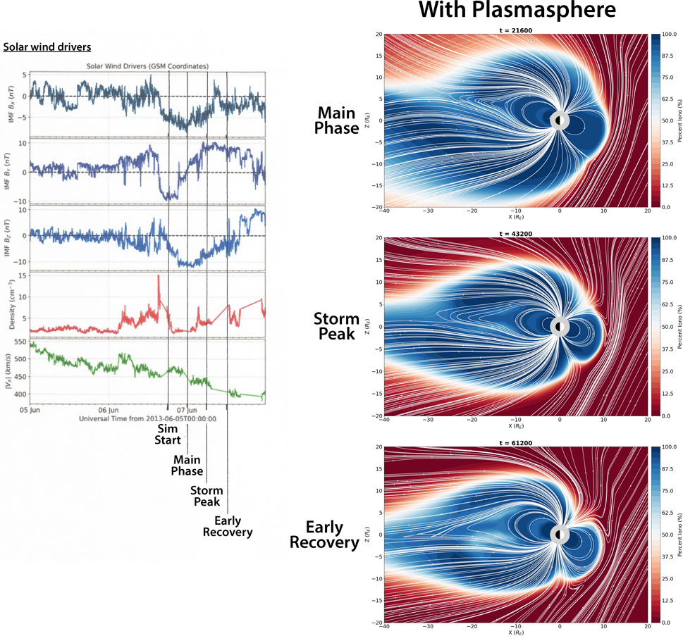
FIGURE 13. Model results on the storm period shown in Figure 12 combining the H+ and O+ contributions of the polar wind and polar cusp (blue) versus the solar wind H+ (red).
The solar wind parameters are shown in the left panel together with the timing of the simulation start followed by the main phase, storm peak and early recovery times in the simulation run shown by the four vertical lines in the solar wind drivers plot. The key Bz component of the solar wind is shown in the third panel down and this component of the solar wind turns southward at 1800 UT on June 6, 2013. This is the starting time of the previously discussed simulation with the ionospheric polar wind and polar cusp plasma flowing out of the ionosphere and through the lobes. In addition to the southward component of the solar wind Bz, the density of the solar wind had increased substantially during the day before the storm (panel 4)
The results are dramatic. The top panel of Figure 13 shows the main phase of the storm. Because of the orientation of the Earth’s spin axis and the dipole axis, the southern hemisphere and lobe are dominated by the polar wind outflow out to greater than 40 RE and the northern hemisphere and lobe are dominated by the polar cusp outflow out to 20 RE. The midplane of the tail has a dominant ionospheric H+ and O+ contribution out to 40 RE and the lobes are full of outflowing ionospheric plasma which can continue to access the midplane in the 24 h while the Bz remains southward continuing to mass load the tail.
In the second panel, the storm peak phase is shown. The ionospheric plasma in the lobes has penetrated into the midplane giving an ionospheric contribution of H+ and O+ that dominates the solar wind in the mid-plane reconnection region of the tail out past 40 RE with a thickness exceeding 10 RE. It is during this time period that the ionospheric ions that were initially flowing in the lobes are energized to keV energies of the warm plasma cloak and plasma sheet reconnection region and subsequently to the 10’s of keV ring current energies, causing the expansion phase of the storm.
In the third panel the recovery phase is shown. The southward Bz component of the solar wind is decreasing and the ionospheric plasma in the lobes is beginning to flow farther down the tail and will begin to exhaust out of the back of the tail as the Bz goes northward. The ionospheric contribution remains dominant throughout the tail region although the solar wind H+ ions are beginning to show up in the inner plasma sheet region (white hazy regions). This ionospheric dominance has been discussed previously by Moore and Delcourt, 1995. It should be remembered that during these changing Bz periods, the ability of the ionospheric ions in the lobes of the tail to reach the midplane in the midnight sector is much faster (10’s of min) than the solar wind ions which must diffuse from the flanks of the tail.
A corollary thought regarding the entry of the low energy lobe plasma into the plasma sheet is the need to understand the processes that are taking place in what has been called the plasma sheet boundary layer. On the north and south outer layers of the plasma sheet, the characteristics of the plasma in the plasma sheet are different closer to the mid-plane than they are at the edges. Data from the MMS spacecraft offer interesting insights into how the transition from lobe plasma to plasma sheet plasma takes place. The energization of the ions as they enter the midplane has been discussed above in Figure 5 and Figure 9. The orbits of the MMS spacecraft permit observations of this plasma sheet/lobe boundary interface.
In the past we have sought to explain this interface in terms of the different ways that the solar wind access can happen, but what may more likely be the case is that this plasma sheet boundary layer is showing us how the lower energy lobe plasma is energized to become the central plasma sheet. Figure 14 shows an MMS orbit for July 15, 2018 in which the lobe/plasma sheet transitions happen several times during the pass. The lower right-hand corner inset figure shows the XZ plane of this MMS orbit which is crossing through the midnight sector at this time. The XZ plane of the orbit is projected on the calculated magnetospheric shape, and shows that the orbit is moving out of the plasma sheet region and into the lobe. When the plasma sheet thins and thickens because of the changing solar wind conditions during the time of passage, MMS can make multiple entries into and out of the lobe.
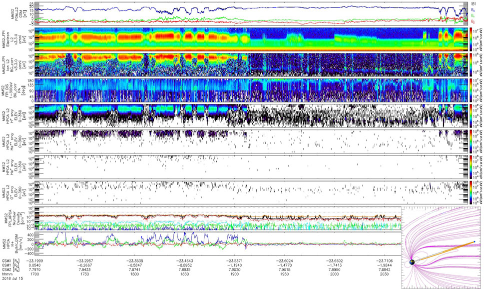
FIGURE 14. A composite picture of MMS data on July 15, 2018 through the plasma sheet boundary layer at the interface of the lobe and plasma sheet.
A look at the 24 h summary plot of MMS data for this orbit (not shown here) displays that there are significant lobe entries at 0100, 0600, 1900 and 2200 UT. We focus here on this expanded plot for the period from 1700 to 2200 UT where the plasma sheet thins, as seen by the dropout of keV electrons and ions at 1900 UT in the second and third panels of the stacked plots, This thinning is in response to an increased X component of the B field as shown by the blue line in the upper first panel. Throughout the time period of 1700–1900 UT as the spacecraft is approaching the northern edge of the plasma sheet from within, this repeated thinning puts the spacecraft alternately in the lobe and then back into the plasma sheet as the plasma sheet thins and then thickens again, multiple times.
These are places where the spacecraft is transitioning from plasma sheet to lobe to plasma sheet and this transition can give us information on the processes that take place at that interface. What can be seen here is that when the spacecraft goes into the lobe, the energy, as measured by the Fast Plasma Instrument in the third of the stacked plots, drops from 1 to 10 keV (plasma sheet) down to about 10–100 eV (lobal winds) and this energy change reverses when the plasma sheet thickens again (decreased X-component of B field).
Kitamura (2019) (GEM) has looked at this particular case in much more detail. The plasma sheet section ends at 1900 UT when the plasma sheet thins and the lobe is encountered by the spacecraft. Then the spacecraft goes back into the plasma sheet at 2100 UT when the plasma sheet thickens again. As was noted above, the first (top) of the stacked plots shows the three components of the magnetic field, the second plot is for the electrons from 10 eV to 10 keV, the third panel is the ions from less than 10 eV to 10 keV. The fourth plot displays the pitch angle distribution of the 1–300 eV ions. The stacked plots below that show the HPCA ion composition measurements integrated over all pitch angles beginning with H+, then He++, then He+, then O+ from 10 eV to 10 keV followed by the number density and the bulk flow velocity.
When the lobe is solidly encountered at 1900 UT, the energies of the ions measured by FPI drop from keV to less than 100 eV. The spacecraft has an ion emitter for potential control. The electrons in the second panel show a similar energy decrease at the lobe encounter. The fourth panel shows the pitch angle distribution for the 1–300 eV ions. In the lobe between 1900 and 2100 UT, these low energy ions are field-aligned at 180° pitch angle which indicates that they are flowing out of the northern ionosphere and flowing through the lobe into the plasma sheet. In the plasma sheet segments (1700–1900 UT) one can still see ions at low energy (panel 4). These are 0–300 eV, but they are now spread over pitch angles of 180 down to 90°. They are picking up perpendicular energy as they come into the plasma sheet region which is compatible with their curvature drift in the cross-tail potential as discussed above in Figure 9.
If we look at the HPCA data in stacked plots 5–8, we see that there is H+ in both the plasma sheet and the lobes. There is He++, which is in the plasma sheet but not in the lobes. The He+ is mostly in the plasma sheet with some in the lobe and the O+ ions are found both in the plasma sheet and the lobe. Initial indication from the He++ is that there is solar wind entry into the plasma sheet. The H+ measurements are ambiguous because of the possibility of both ionospheric and solar wind sources although their energies are much lower in the lobe, as expected for their polar wind source and they are energized in the plasma sheet region. There is O+ in both the lobe and the plasma sheet that probably comes from the polar cusp through the lobes and possibly from the nightside auroral zone source. This single case suggests that very valuable information can be learned from MMS about the lobe/plasma sheet transition region which is found at the plasma sheet boundary layer and what it can show concerning the sources and processes that fill the plasma sheet.
In the previous sections we have shown how the ionosphere is capable of being the dominant source for the different plasma regions of the magnetosphere, based on observations of the outflowing plasma from the ionosphere and the processes that can move it and energize it to create the energetic plasma regions. The evidence for the ionosphere as a source is quite compelling based on both measurement and multi-fluid merged modeling.
We now examine how the outflowing ionospheric plasma can load the magnetosphere based on the changing Bz of the solar wind. We have shown the magnitude of the outflow and how it can move through the lobes of the tail to populate the plasma sheet, the principal region for reconnection in the magnetotail. We have also shown that the ionospheric outflow is affecting the magnetosphere from the inside-out and its omnipresence in the magnetotail lobes in the midnight sector gives it fast access (10’s of min) to the plasma sheet region in contrast to the solar wind plasma entry which can take an hour or more to reach and begin to enter the flanks of the plasma sheet. The merged ionosphere/magnetosphere MHD modeling shown in Figure 12 and Figure 13 illustrates how the ionospheric outflow can load the magnetosphere sufficiently enough to create the plasma sheet and ring current in contrast to the solar wind.
The dynamics of the ionospheric source in combination with the changing solar wind Bz and with the different access and energization times for the ionosphere and solar wind plasma suggest a new or modified model for the initiation of substorms and storms in the magnetosphere. Figure 15 illustrates the new model and serves as a basis by which we can examine how these dynamic magnetospheric processes might be triggered.
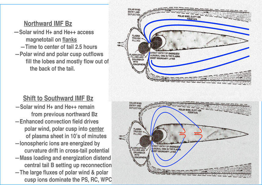
FIGURE 15. Two sketches which give a schematic picture of the suggested process by which ionospheric and solar wind plasma access the magnetospheric tail and through which the ionosphere can be a dominant plasma source and a driver of magnetospheric storms and substorms.
The timing considerations discussed above suggest that following the Bz southward turning of the solar wind magnetic field, the ionospheric source is poised to access the plasma sheet in tens of minutes and become energized in minutes, thus mass-loading the tail and distending the magnetic field lines in the neutral sheet. The entry and energization of the outflowing ionospheric plasma in the lobes establishes a changed environment in the plasma sheet that is very favorable for reconnection to begin, thus initiating substorms and storms. The availability and quick access of the ionospheric-origin plasma to the midnight sector neutral sheet in contrast to the access times required by the solar wind H+ establishes the ionosphere together with the solar wind southward Bz as major components of the driving mechanism in the process of magnetospheric dynamics.
Figure 15 is a sketch which illustrates two time periods. In the upper panel the pre-storm northward Bz period is shown in which the solar wind is supplying plasma to the flanks of the tail as discussed above (Sorathia et al., 2019). In the lower panel the time period following the change of the solar wind Bz to southward is shown.
Beginning with the top panel, during a northward Bz, the solar wind plasma has been accessing the plasma sheet region with H+ and He++ into the magnetotail on the flanks. The total solar wind access time from the bow shock in towards the center of the tail is about two and a half hours. The polar wind and polar cusp outflows move as shown by the blue lines through the lobes. There is no convection field, and a very small cross-tail potential if any, and the streaming ions flow almost entirely (90%) out of the tail of the magnetosphere (Haaland et al., 2012). These ionospheric polar wind and polar cusp low energy ions do not affect the plasma sheet significantly during northward Bz.
Then as illustrated in the lower panel, when the solar wind Bz turns southward, the H+ and He++ solar wind ions that had entered the tail during the period of northward Bz remain there while the ions that are streaming outward in the lobes and down the tail have their trajectories dramatically altered by the increased convection electric field and are driven into the plasma sheet region quickly in 10’s of min. These H+, He+ and O+ ionospheric ions can enter quickly because they had flowed out to their positions in the tail during the previous northward Bz time period and only have to drift a short distance to reach the plasma sheet region. This begins to mass-load the neutral sheet field lines and distend/stretch them further. This increases their curvature and increases the energization of the entering lobe particles to keV energies through their curvature drift across the tail and the energization that comes from the cross-tail potential which has also been increased because of the southward turning solar wind Bz. These entering ions can gain their keV energies in about 10 min after they enter the region of distended field lines (see Figure 9) improving the environment for reconnection to begin. With the southward Bz occurring, about 90% of these lobe ions will enter the plasma sheet region instead of flowing out of the back of the tail (Haaland et al., 2012). The stronger the southward Bz, the closer to the earth the lobe ions are pushed into the plasma sheet.
The large fluxes of polar wind and polar cusp ions, once energized, dominate the plasma sheet and flow earthward creating the ring current, and the warm plasma cloak. This is a very different way of thinking about a substorm or a storm. Solar wind Bz is still the trigger, but the particles are dominantly delivered by the ionosphere through the lobes.
It is important to note that the dynamics in the magnetotail may not only be due to steady convection and laminar flows, but can have a major contribution from turbulence and mesoscale structures. It was noted early on that injections from the magnetotail can contribute to ring current build up (Parks and Winckler, 1968). Indeed, recent numerical simulations suggest that the contribution of bursty flows in the plasma sheet can contribute much of the ring current build up (Yang et al., 2015). This picture is consistent with observations showing that bursty bulk flows (BBF’s) can account for much of mass and energy transport in the plasma sheet (Angelopoulos et al., 1994). The potentially bursty nature of this transport can have important implications for the energization of particles in the tail, including ionospheric particles which reach the equatorial plane from the lobes. In particular, bursty transport means that some of the particle energization may be non-adiabatic. For O+ especially, which has a large gyroradius, there are indications in observations that non-adiabatic acceleration associated with fast flows can be important (Keika et al., 2010, 2013). Regardless of whether the transport is bursty or laminar in the tail, acceleration of particles of ionospheric origin reaching down tail will occur, albeit the details of the transport may change. Additionally, just as the transport in the magnetosphere can have important contributions from fast flows and mesoscale structures, the outflow itself can be significantly structured. For instance, Schunk et al., 2005 showed that one can have localized propagating patches of polar wind outflow. The contributions of such structure in the outflow in combination with the bursty nature of the transport are certainly worthy of continued study.
Here is the storm process in summary. Northward Bz has solar wind ions contributing to the plasma sheet and the ionospheric plasma, polar wind and polar cusp fills the lobes but is flowing out of the back of the tail. The growth phase occurs when Bz turns southward and the lobe outflows are convected into the mid-plane where they are energized in tens of minutes and stretch the tail. The distended tail increases the curvature drift and the cross-tail potential further energizes the formerly ionospheric ions. Then, when the tail is loaded, reconnection begins and makes the expansion phase. This is the area that is being studied extensively in detail for reconnection events by MMS spacecraft and the ionospheric source plays a significant role in creating this plasma reconnection region. The reconnection starts the aurora, which starts the ionospheric currents flowing, changes them, and gives the familiar magnetic signatures in the auroral zone.
Then the newly created and energized plasma sheet flows earthward and is further energized. The ring current strengthens so that the total of the polar wind H+ and polar cusp O+ are dominant in it over the solar wind H+ (Glocer et al., 2020). A large storm can develop and continue as long as the southward solar wind Bz is there because the ionosphere is sending out polar wind and polar cusp ions continuously, and as long as the Bz delivers these ions to the mid-plane, the storm can continue. When Bz goes back northward again, the lobal wind begins to exhaust out the back of the tail and the storm ends.
What do we know? The ionospheric plasma plays a major role in populating the magnetosphere and affecting its dynamics. The initially cold (few eV) ionospheric plasma creates the polar wind, which fills the plasmasphere and the plasma trough, and creates the dense detached plasma and plumes that drift from the duskside plasmapause out to the magnetopause, which affects the reconnection rate there. At higher latitudes outside of the plasmasphere, the polar wind flows upward supersonically, dominated by cold H+ and He+ and together with the outflowing polar cusp plasma of H+, He+ and O+ is convected across the polar cap to fill the lobes of the magnetotail continuously.
As the polar wind and polar cusp outflows move through the lobes, they can be convected into the mid-plane of the magnetotail to be a major contributor to the creation of the plasma sheet, the ring current and the warm plasma cloak. In addition, the lower latitude plasmasphere and plasma trough cold plasma drives wave-particle interactions that both create and determine the propagation of waves that are a dominant influence on the creation of the radiation belts.
Together with the solar wind IMF Bz, the ionospheric plasma is a major driver of substorms and major storms when the southward Bz convects the copius outflowing cold plasma in the lobes into the central plasma sheet region, mass-loading this region, distending the magnetospheric field lines in the neutral sheet, energizing the cold plasma to plasma sheet energies and setting up the reconnection process which results in substorms and storms.
Both the cold unaccelerated plasma of the plasmasphere and the accelerated outflowing ionospheric plasma of the warm plasma cloak influence the strength of the reconnection at the nose of the magnetosphere. In addition, both the unaccelerated polar wind outflow and the accelerated ionospheric lobal wind together with the accelerated ionospheric plasma sheet create a dominant element of the environment in which reconnection happens in the central plasma sheet of the magnetotail. The plasma sheet boundary layer is the transition layer where the cold outflowing lobe plasma is transformed into the hot plasma sheet plasma and warm plasma cloak regions.
Recently created merged ionosphere/magnetosphere multi-fluid MHD models are able to differentiate between the H+ ions which come from the ionosphere in the polar wind and polar cusp from the H+ ions that enter the magnetosphere from the solar wind. This otherwise unmeasurable difference has given invaluable new insight into the relative strength of these two magnetospheric plasma sources and their relative ability to drive substorms and storms.
What do we need to know? New measurements of the composition of the ionospheric outflow, and the resulting ion trajectories and energization of this outflow must be carried out together with the advancement of merged multi-fluid models of the ionosphere and magnetosphere that can clearly differentiate between ionospheric H+ and solar wind H+. These merged multi-fluid models will be our roadmap to track the pathways that cold ions and electrons follow as they move through the magnetosphere, are energized and create the distinctive magnetospheric plasma regions that we have observed for decades but have not fully understood—the magnetosphere tapestry.
The merged models together with ion trajectory models are needed in order to allow us to understand the observations in the lobe, plasma sheet boundary layer, central plasma sheet, ring current and warm plasma cloak. These new merged models should be expanded to include more multi-fluids in addition to the ionospheric and solar wind H+. They should add particularly He++ and O6+ from the solar wind as well as O+, He+, N+, O++, and NO+ from the ionosphere.
In summary, what are our next steps? We need to try to understand how the ions and electrons actually move through and are energized to make the principal regions of the magnetosphere and how changes in the solar wind Bz can cause a storm to occur there. The low energy electrons are even more difficult to measure accurately than the ions because of spacecraft charging and photoelectron emission from the spacecraft surface. We should continue to develop the multi-ion capabilities of the merged multi-fluid models that can separate the solar wind H+ from the ionospheric H+ in order to interpret the ion observations. There will be much significant new information that comes from running these multi-fluid models and comparing with the evolving ion trajectory observations.
We must also start again to fly missions that have specific separate instrumentation with large geometric factors that will give the sensitivity required to measure individual initially cold, few eV, ion phase space densities and how they are transformed as they move through the magnetosphere. These highly sensitive differential angle instruments which include composition must be accompanied by a successful plasma neutralizing device that can keep the spacecraft potential close to plasma potential without interfering with other measurements on the spacecraft.
Finally, new missions must be selected and flown which measure the composition, energy and angular distribution of all of the areas of outflow from the Earth’s ionosphere, which become the very significant source of the distinctive regions of the magnetosphere. In addition, these missions should utilize the highly sensitive low to medium energy measurements to track the 100’s of eV to 100 keV ion trajectories of the source ions and electrons as they are energized to populate the magnetosphere hot plasma regions and drive the substorms and storms.
We will be able to use the merged multifluid models as a roadmap to help understand what we are observing in the particles. The merged models using those additional ions and the particle tracing will help us determine the ion pathways and unravel the origin of the particle measurements. They will also allow us to understand how the environment for reconnection is created in the plasma sheet and at the magnetopause.
All authors listed have made a substantial, direct, and intellectual contribution to the work and approved it for publication
The authors declare that the research was conducted in the absence of any commercial or financial relationships that could be construed as a potential conflict of interest.
All claims expressed in this article are solely those of the authors and do not necessarily represent those of their affiliated organizations, or those of the publisher, the editors and the reviewers. Any product that may be evaluated in this article, or claim that may be made by its manufacturer, is not guaranteed or endorsed by the publisher.
This paper is dedicated to Don Carpenter at Stanford University and Ed Shelley at the Lockheed Palo Alto Research Laboratory. One of us (CRC) had the privilege of working with Don and Ed when he went to Lockheed in Palo Alto. Don showed us the presence of ionospheric plasma in the magnetosphere, the plasmasphere, Carpenter’s knee. Ed showed us that one can see O+ in the magnetosphere that has keV energies that obviously came from the Earth’s ionosphere and subsequently got energized. Our community has been, to a certain degree, not completely following through on what Ed showed us because we know that O+ is from the ionosphere but we have tended to overlook the fact that the ionosphere is also putting copius amounts of H+ into the magnetosphere; we have just never been able to tell it apart from the solar wind H+ which we now can and certainly should do. One of us (CRC) would also like to thank his thesis advisor, Brian O'Brien, who has left his scientific imprints in the Earth’s magnetosphere and on the moon and Martin Walt, who is the scientist leader who enabled him to come to Lockheed as a green PhD and gave him the opportunity to do work in these many different fascinating areas of magnetospheric physics. Rick was also able to meet Andy Nagy, Peter Banks and Bill Hanson and began learning about the ionosphere from them. Many thanks go to Stan Fields, David Reasoner, Bill Lewter and Bill Baker at MSFC for building the RIMS instrument for Dynamics Explorer satellite together with the University of Michigan and the University of Texas at Dallas and later to Thom Moore, Stan Fields and Nobie Stone at NASA/Marshall Space Flight Center as well as Jean-Jacques Berthelier at CNRS and Dave Young at SwRI, to build the TIDE instrument for the Polar satellite. Thanks also go to all of the members of the magnetospheric branch at the NASA/Marshall Space Flight Center for their important and essential contributions to the analysis of the RIMS and TIDE data. This research was supported by the National Aeronautics and Space Administration, Magnetospheric Multiscale Mission (MMS) in association with NASA contract NNG04EB99C.
Abe, T., Watanabe, S., Whalen, B. A., Yau, A. W., and Sagawa, E. (1996). Observations of Polar Wind and thermal Ion Outflow by Akebono/SMS. J. Geomagn. Geoelec 48, 319–325. doi:10.5636/jgg.48.319
André, M., and Cully, C. M. (2012). Low-Energy Ions: A Previously Hidden Solar System Particle Population. Geophys. Res. Lett. 39, L03101. doi:10.1029/2011gl050242
André, M., and Yau, A. (1997). Theories and Observations of Ion Energization and Outflow in the High Latitude Magnetosphere. Space Sci. Rev. 80 (27), 27–48. doi:10.1007/978-94-009-0045-5_2
Angelopoulos, V., Kennel, C. F., Coroniti, F. V., Pellat, R., Kivelson, M. G., Walker, R. J., et al. (1994). Statistical Characteristics of Bursty Bulk Flow Events. J. Geophys. Res. 99 (21), 21257. doi:10.1029/94ja01263
Banks, P. M., and Holzer, T. E. (1968). The Polar Wind. J. Geophys. Res. 73, 6846–6854. doi:10.1029/ja073i021p06846
Banks, P. M., Nagy, A. F., and Axford, W. I. (1971). Dynamical Behavior of Thermal Protons in the Mid-latitude Ionosphere and Magnetosphere. Planet. Space Sci. 19 (9), 1053–1067. doi:10.1016/0032-0633(71)90104-8
Barakat, A. R., and Schunk, R. W. (2006). A Three-Dimensional Model of the Generalized Polar Wind. J. Geophys. Res. 111 (A12), 1978. doi:10.1029/2006ja011662
Brambles, O. J., Lotko, W., Damiano, P. A., Zhang, B., Wiltberger, M., and Lyon, J. (2010). Effects of Causally Driven Cusp O+ Outflow on the Storm Time Magnetosphere-Ionosphere System Using a Multifluid Global Simulation. J. Geophys. Res. 115, n/a. doi:10.1029/2010ja015469
Carpenter, D. L. (1963). Whistler Evidence of a “Knee” in the Magnetospheric Ionization Density Profile. J. Geophys. Res. 68, 1675. doi:10.1029/jz068i006p01675
Chandler, M. O., Moore, T. E., and Waite, J. H. (1991). Observations of Polar Ion Outflows. J. Geophys. Res. 96, 1412. doi:10.1029/90ja02180
Chappell, C. R., Fields, S. A., Baugher, C. R., Hoffman, J. H., Hanson, W. B., Wright, W. W., et al. (1981). The Retarding Ion Mass Spectrometer on Dynamics Explorer-A. Space Sci. Instrum. 5, 477.
Chappell, C. R., Giles, B. L., Moore, T. E., Delcourt, D. C., Craven, P. D., and Chandler, M. O. (2000). The Adequacy of the Ionospheric Source in Supplying Magnetospheric Plasma. J. Atmosph.Solar-Terrestr. Phys. 62, 421. doi:10.1016/s1364-6826(00)00021-3
Chappell, C. R., Huddleston, M. M., Moore, T. E., Gilse, B. L., and Delcourt, D. C. (2008). Observations of the Warm Plasma Cloak and an Explanation of its Formation in the Magnetosphere. J. Geophys. Res. 113, A09206. doi:10.1029/2007ja012945
Chappell, C. R., Moore, T. E., and Waite, J. H. (1987). The Ionosphere as a Fully Adequate Source of Plasma for the Earth’s Magnetosphere. J. Geophysic. Res. 92, 5896. doi:10.1029/ja092ia06p05896
Chappell, C. R. (1972). Recent Satellite Measurements of the Morphology and Dynamics of the Plasmasphere. Rev. Geophys. Space Phys. 10 (4), 951. doi:10.1029/rg010i004p00951
Cladis, J. B. (2000). Obserations of Centrifugal Acceleration during Compression of Magnetosphere. Geophys. Res. Lett. 27, 915. doi:10.1029/1999gl010737
Cladis, J. B. (1986). Parallel Acceleration and Transport of Ions from Polar Ionosphere to Plasma Sheet. Geophys. Res. Lett. 13, 893. doi:10.1029/gl013i009p00893
Cully, C. M., Donovan, E. F., Yau, A. W., and Arkos, G. G. (2003a). Akebono/Suprathermal Mass Spectrometer Observations of Low-Energy Ion Outflow: Dependence on Magnetic Activity and Solar Wind Conditions. J. Geophys. Res. 108, 1093. doi:10.1029/2001ja009200
Cully, C. M., Donovan, E. F., Yau, A. W., and Opgenoorth, H. J. (2003b). Supply of Thermal Ionospheric Ions to the Central Plasma Sheet. J. Geophys. Res. 108, 1092. doi:10.1029/2002ja009457
Delcourt, D. C., Moore, T. E., and Chappell, C. R. (1994). Contribution of Low-Energy Ionospheric Protons to the Plasma Sheet. J. Geophys. Res. 99 (A4), 5681. doi:10.1029/93ja02770
Delcourt, D. C., Sauvaud, J. A., and Moore, T. E. (1993). Polar Wind Ion Dynamics in the Magnetotail. J. Geophys. Res. 98, 9155. doi:10.1029/93ja00301
Engwall, E., Eriksson, A. I., Cully, C. M., Andre, M., Puhl-Quinn, P. A., Vaith, H., et al. (2009a). Survey of Cold Ionospheric Outflows I the Magnetotail. Ann. Geophys. 27, 3185. doi:10.5194/angeo-27-3185-2009
Engwall, E., Eriksson, A. I., Cully, C. M., Andre, M., Torbert, R., and Vaith, H. (2009b). Earth’s Ionospheric Outflow Dominated by Hidden Cold Plasma. Nat. Geosci 2 (24), 24–27. doi:10.1038/ngeo387
Engwall, E., Eriksson, E. I., Andre, M., Dandouras, I., Paschmann, G., Quinn, J., et al. (2006). Low- Energy (Order 10 eV) Ion Flow in the Magnetotail Lobes Inferred from Spacecraft Wake Observations. Geophys. Res. Lett. 33, 6110. doi:10.1029/2005gl025179
Fok, M.-C. (1999). Storm Time Modeling of the Inner Plasma Sheet/Outer Ring Current. J. Geophys. Res. 104, 14557. doi:10.1029/1999ja900014
Fuselier, S. A., Mukherjee, J., Denton, M. H., Petrinec, S. M., Trattner, K. J., Toledo-Redondo, S., et al. (2019). High-Density O+ in Earth’s Outer Magnetosphere and its Effect on Dayside Magnetopause Magnetic Reconnection. JGR Space Phys. 124, 10257–10269. doi:10.1029/2019JA027396
Giles, B. L., Chappell, C. R., Moore, T. E., Comfort, R. H., and Waite, J. H. (1994). Statistical Survey of Pitch Angle Distributions in Core (0-50 eV) Ions from Dynamics Explorer 1: Outflow in the Auroral Zone, Polar Cap, and Cusp. J. Geophys. Res. 99 (17), 483. doi:10.1029/94JA00864
Glocer, A., Tóth, G., Gombosi, T., and Welling, D. (2009). Modeling Ionospheric Outflows and Their Impact on the Magnetosphere: Initial Results. J. Geophys. Res. 114, A05216. doi:10.1029/2009ja014053
Gringauz, K. I. (1963). The Structure of the Ionized Gas Envelope of Earth from Direct Measurements in the USSR of Local Charged Particle Concentrations. Planet. Space Sci. 11, 281. doi:10.1016/0032-0633(63)90030-8
Gurgiolo, C., and Burch, J. L. (1982). DE-1 Observations of the Polar Wind—A Heated and an Unheated Component. Geophys. Res. Lett. 9, 945. doi:10.1029/gl009i009p00945
Haaland, S., Eriksson, A., Engwall, E., Lybekk, B., Nilsson, H., Pedersen, A., et al. (2012). Estimating the Capture and Loss of Cold Plasma from Ionospheric Outflow. J. Geophys. Res. 117, A07311. doi:10.1029/2012ja017679
Harris, K. K., and Sharp, G. W. (1969). Ogo 5 Ion Spectrometer. Trans. IEEE Geosci. Electron. 7 (2), 93. doi:10.1109/tge.1969.271328
Hoffman, J. H. (1970). Studies of the Composition of the Ionosphere with a Magnetic Deflection Mass Spectrometer. Int. J. Mass. Spectrom. Ion Phys. 4, 315–322. doi:10.1016/0020-7381(70)85047-1
Horwitz, J. L., Ho, C. W., Scarbro, H. D., Wilson, G. R., and Moore, T. E. (1994). Centrifugal Acceleration of the Polar Wind. J. Geophys. Res. 99 (15), 051. doi:10.1029/94JA00924
Huddleston, M. M., Chappell, C. R., Delcourt, D. C., Moore, T. E., Giles, B. L., and Chandler, M. O. (2005). An Examination of the Process and Magnitude of Ionospheric Plasma Supply to the Magnetosphere. J. Geophys. Res. 110 (12), 202. doi:10.1029/2004ja010401
Keika, K., Brandt, P. C., Ohtani, S., Mitchell, D. G., Min, K., Nose, M., et al. (2010). Mass-Independent Evolution of Energetic Neutral Atoms Energy Spectra During Storm Time Substorms: Implication for O+ Nonadiabatic Acceleration. J. Geophys.Res: Space Phys. 115, A00I12. doi:10.1029/2010ja015889
Keika, K., Kistler, L. M., and Brandt, P. C. (2013). Energization of O+ Ions in the Earth’s Inner Magnetosphere and the Effects on Ring Current Buildup: A Review of Previous Observations and Possible Mechanisms. J. Geophys. Res:space Phys. 118, 4441. doi:10.1002/jgra.50371
Kistler, L. M., Mouikis, C. G., Klecker, B., and Dandouras, I. (2010). Cusp as a Source for Oxygen in the Plasma Sheet during Geomagnetic Storms. J. Geophys. Res. 115, A03209. doi:10.1029/2009ja014838
Kitamura, N. (2019). Cold Ion Observations by MMS at the Lobe and Near PSBL. Santa Fe, NM: GEM Meeting.
Liao, J., Kistler, L. M., Mouikis, C. G., Klecker, B., Dandouras, I., and Zhang, J.-C. (2010). Statistical Study of O+ Transport from the Cusp to the Lobes with Cluster CODIF Data. J. Geophys. Res. 115, A00J15. doi:10.1029/2010ja015613
Liemohn, M. W., Moore, T. E., Craven, P. D., Maddox, W., Nagy, A. F., and Kozyra, J. U. (2005). Occurrence Statistics of Cold, Streaming Ions in the Near-Earth Magnetotail: Survey of Polar-TIDE Observations. J. Geophys. Res. 110, A07211. doi:10.1029/2004ja010801
Lockwood, M., Waite, J. H., Moore, T. E., Johnson, J. F. E., and Chappell, C. R. (1985). A New Source of Suprathermal O+ Ions Near the Dayside Polar Cap Boundary. J. Geophys. Res. 90, 4099. doi:10.1029/ja090ia05p04099
Moore, T. E., Chappell, C. R., Chandler, M. O., Craven, P. D., Giles, B. L., Pollock, C. J., et al. (1997). High Altitude Observations of the Polar Wind. Science 277, 349. doi:10.1126/science.277.5324.349
Moore, T. E., Chappell, C. R., Chandler, M. O., Fields, S. A., Pollock, C. J., Reasoner, D. L., et al. (1995). The Thermal Ion Dynamics Experiment and Plasma Source Instrument. Space Sci. Revs 71, 409. doi:10.1007/bf00751337
Moore, T. E., Fok, M.‐C., Chandler, M. O., Chappell, C. R., Christon, S. P., Delcourt, D. C., et al. (2005). Plasma Sheet and (Nonstorm) Ring Current Formation from Solar and Polar Wind Sources. J. Geophys. Res. 110, A02210. doi:10.1029/2004ja010563
Mouikis, C. G., Kistler, L. M., Liu, Y. H., Klecker, B., Korth, A., and Dandouras, I. (2010). H+ and O+ Content of the Plasma Sheet at 15-19 Re as a Function of Geomagnetic and Solar Activity. J. Geophys. Res. 115, A00J16. doi:10.1029/2010ja015978
Nagai, T., Waite, J. H., Green, J. L., Chappell, C. R., Olsen, R. C., and Comfort, R. H. (1984). First Measurements of Supersonic Polar Wind in the Polar Magnetosphere. Geophys. Res. Lett. 11, 669. doi:10.1029/gl011i007p00669
Parks, G. K., and Winckler, J. R. (1968). Acceleration of Energetic Electrons Observed at the Synchronous Altitude during Magnetospheric Substorms. J. Geophys. Res. 73, 5786. doi:10.1029/ja073i017p05786
Schunk, R. W., Demars, H. G., and Soijka, J. J. (2005). Propagating Polar Wind Jets. JASTP 67, 357–364. doi:10.1016/j.jastp.2004.09.005
Schunk, R. W., and Sojka, J. J. (1997). Global Ionosphere-Polar Wind System during Changing Magnetic Activity. J. Geophys. Res. 102 (11), 62. doi:10.1029/97ja00292
Shelley, E. G., Johnson, R. G., and Sharp, R. D. (1972). Satellite Observations of Energetic Heavy Ions during a Geomagnetic Storm. J. Geophys. Res. 77, 6104. doi:10.1029/ja077i031p06104
Shelley, E. G., Peterson, W. K., Ghielmetti, A. G., and Geiss, J. (1982). The Polar Ionosphere as a Source of Energetic Magnetospheric Plasma. Geophys. Res. Ltrs. 9 (9), 941–944. doi:10.1029/gl009i009p00941
Sorathia, K. A., Merkin, V. G., Ukhorskiy, A. Y., Allen, R. C., Nykyri, K., and Wing, S. (2019). Solar Wind Ion Entry into the Magnetosphere during Northward IMF. J. Geophys. Res. 124, 5461–5481. doi:10.1029/2019JA026728
Strangeway, R. J., Ergun, E. R., Su, Y.-J., Carlson, C. W., and Elphic, R. C. (2005). Factors Controlling Ionospheric Outflows as Observed at Intermediate Altitudes. J. Geophys. Res. 110, A03221. doi:10.1029/2004JA010829
Su, Y. J., Horwitz, J. L., Moore, T. E., Giles, B. L., Chandler, M. O., Craven, P. D., et al. (1998). Polar Wind Survey with the Thermal Ion Dynamics Experiment/Plasma Source Instrument Suite Aboard POLAR. J. Geophys. Res. 103 (29), 29305–29337. doi:10.1029/98ja02662
Toledo-Redondo, S., André, M., Aunai, N., Chappell, C. R., Dargent, J., Fuselier, S. A., et al. (2021). Impacts of Ionospheric Ions on Magnetic Reconnection and Earth’s Magnetosphere Dynamics. Rev. Geophys. 59, e2020RG000707. doi:10.1029/2020RG000707
Tsyganenko, N. A. (1989). A Magnetospheric Magnetic Field Model with a Warped Tail Current Sheet, Planet. Space Sci. 37, 5.
Welling, D. T., and Ridley, A. J. (2010). Exploring Sources of Magnetospheric Plasma Using Multispecies MHD. J. Geophys. Res. 115, A04201. doi:10.1029/2009ja014596
Welling, D. T., Jordanova, V. K., Zaharia, S. G., Glocer, A., and Toth, G. (2011). The Effects of Dynamic Ionospheric Outflow on the Ring Current. J. Geophys. Res. 116, n/a. doi:10.1029/2010ja015642
Winglee, R. M. (2000). Mapping of Ionospheric Outflows into the Magnetosphere for Varying IMF Conditions. J. Atmos. Terr. Phys. 62, 527. doi:10.1016/s1364-6826(00)00015-8
Yau, A. W., and Andre, M. (1997). Sources of Ion Outflow in the High Latitude Ionosphere. Space Sci. Rev. 80 (1), 1–25. doi:10.1007/978-94-009-0045-5_1
Keywords: ionospheric source, magnetospheric plasma, magnetospheric dynamics, magnetospheric substorms and storms, cold ionospheric ions becoming energized in the magnetosphere
Citation: Chappell CR, Glocer A, Giles BL, Moore TE, Huddleston MM and Gallagher DL (2021) The Key Role of Cold Ionospheric Ions As a Source of Hot Magnetospheric Plasma and As a Driver of the Dynamics of Substorms and Storms. Front. Astron. Space Sci. 8:746283. doi: 10.3389/fspas.2021.746283
Received: 23 July 2021; Accepted: 28 September 2021;
Published: 21 October 2021.
Edited by:
Joseph Eric Borovsky, Space Science Institute, United StatesReviewed by:
Binbin Ni, Wuhan University, ChinaCopyright © 2021 Chappell, Glocer, Giles, Moore, Huddleston and Gallagher. This is an open-access article distributed under the terms of the Creative Commons Attribution License (CC BY). The use, distribution or reproduction in other forums is permitted, provided the original author(s) and the copyright owner(s) are credited and that the original publication in this journal is cited, in accordance with accepted academic practice. No use, distribution or reproduction is permitted which does not comply with these terms.
*Correspondence: C. R. Chappell, cmljay5jaGFwcGVsbEB2YW5kZXJiaWx0LmVkdQ==
Disclaimer: All claims expressed in this article are solely those of the authors and do not necessarily represent those of their affiliated organizations, or those of the publisher, the editors and the reviewers. Any product that may be evaluated in this article or claim that may be made by its manufacturer is not guaranteed or endorsed by the publisher.
Research integrity at Frontiers
Learn more about the work of our research integrity team to safeguard the quality of each article we publish.