Quasinormal Frequencies of a Two-Dimensional Asymptotically Anti-de Sitter Black Hole of the Dilaton Gravity Theory

We numerically calculate the quasinormal frequencies of the Klein-Gordon and Dirac fields propagating in a two-dimensional asymptotically anti-de Sitter black hole of the dilaton gravity theory. For the Klein-Gordon field we use the Horowitz-Hubeny method and the asymptotic iteration method for second order differential equations. For the Dirac field we first exploit the Horowitz-Hubeny method. As a second method, instead of using the asymptotic iteration method for second order differential equations, we propose to take as a basis its formulation for coupled systems of first order differential equations. For the two fields we find that the results that produce the two numerical methods are consistent. Furthermore for both fields we obtain that their quasinormal modes are stable and we compare their quasinormal frequencies to analyze whether their spectra are isospectral. Finally we discuss the main results.

1 Introduction

The quasinormal modes (QNMs) are the oscillations of perturbed black holes that are purely ingoing near the horizon. The boundary condition imposed at the asymptotic region depends on its structure, for example, for asymptotically flat black holes the boundary condition usually imposed is that the perturbation is purely outgoing as r → ∞, whereas for the asymptotic anti-de Sitter black holes (asymptotically adS black holes, in what follows), a common boundary condition demands that the perturbation goes to zero as r → ∞ (Avis et al., 1978; Kokkotas and Schmidt, 1999; Berti et al., 2009; Konoplya and Zhidenko, 2011). It is convenient to notice that in asymptotically adS spacetimes we can impose a different boundary condition as r → ∞. See Refs. (Breitenlohner and Freedman, 1982; Burgess and Lütken, 1985; Dasgupta, 1999) for some examples. Associated with the QNMs we find a set of complex frequencies called quasinormal frequencies (QNFs). It is well known that the QNFs of black holes are determined by the geometry and the type of perturbation (Kokkotas and Schmidt, 1999; Berti et al., 2009; Konoplya and Zhidenko, 2011).

Two dimensional gravity allows us to analyze several physical problems in a simple framework. The physical properties of two-dimensional black holes (2D black holes, in what follows) are studied because some aspects of the analysis are simpler than in spacetimes with D ≥ 3 dimensions (Grumiller et al., 2002; Grumiller and Meyer, 2006). Furthermore, in 2D spacetimes the equations of motion for classical fields simplify and we can study in more detail several physical phenomena, for example, the way in which a 2D black hole reacts when it is perturbed. The QNFs of 2D spacetimes have been studied in recent times (Li et al., 2001; Kettner et al., 2004; Becar et al., 2007; Zelnikov, 2008; López-ortega, 2009; Becar et al., 2010; López-ortega, 2011; López-Ortega and Vega-Acevedo, 2011; Cordero et al., 2012; Myung and Moon, 2012; Estrada-Jiménez et al., 2013; Stetsko, 2017; Jusufi et al., 2018; Sakallı et al., 2018; Mirbabayi, 2020; Bhattacharjee et al., 2021; Kanzi and Sakallı, 2021; Sakalli and Tokgöz Hyusein, 2021). Exact results for the QNFs have previously found (Li et al., 2001; Kettner et al., 2004; Becar et al., 2007; Zelnikov, 2008; López-ortega, 2009; Becar et al., 2010; López-ortega, 2011; López-Ortega and Vega-Acevedo, 2011; Cordero et al., 2012; Myung and Moon, 2012; Estrada-Jiménez et al., 2013; Stetsko, 2017; Jusufi et al., 2018; Sakallı et al., 2018; Mirbabayi, 2020; Bhattacharjee et al., 2021; Kanzi and Sakallı, 2021; Sakalli and Tokgöz Hyusein, 2021), but for some asymptotically adS 2D backgrounds a numerical calculation is necessary (Cordero et al., 2012).

We notice that the QNFs of asymptotically adS black holes have attracted attention, since they are useful to study its classical stability (Chan and Mann, 1997; Chan and Mann, 1999; Kokkotas and Schmidt, 1999; Horowitz and Hubeny, 2000; Giammatteo and Jing, 2005; Berti et al., 2009; Lopez-Ortega, 2010; Konoplya and Zhidenko, 2011; Cordero et al., 2012) and to calculate the entropy spectrum of the black hole horizon (Hod, 1998; Maggiore, 2008; Wei and Liu, 2009; Kwon and Nam, 2010; López-Ortega, 2010). Here we exploit the advantages that we find in 2D gravity to implement two numerical methods to calculate the QNFs of a 2D asymptotically adS black hole (Lemos and Sá, 1994). Additionally, we carry out this work to understand the properties of this 2D black hole of Lemos and Sá (1994) and study its classical stability under small perturbations. One of the numerical procedures is the widely used Horowitz-Hubeny method (HH method in what follows) (Horowitz and Hubeny, 2000) that is appropriate to compute the QNFs of asymptotically adS spacetimes (Berti et al., 2009; Konoplya and Zhidenko, 2011). The other numerical procedure is the asymptotic iteration method (AIM in what follows) (Ciftci et al., 2003), that is modified to determine the QNFs of black holes (Cho et al., 2010). For the Klein-Gordon field the AIM is exploited in the usual formulation for second order differential equations (Ciftci et al., 2003; Cho et al., 2010), whereas for the Dirac field we propose to use the formulation of the AIM for coupled systems of first order differential equations (Ciftci et al., 2005). As far as we know, this version of the AIM has not previously used to calculate QNFs of black holes and we think that the computation of the QNFs for 2D black holes is the appropriate setting to test this method.

The rest of the paper is structured as follows. In Section 2.1 we give the asymptotically adS 2D black hole that we study in this work and we describe its main properties. In Section 2.2 we simplify the equation of motion for the Klein-Gordon field in the 2D black hole that we study. Furthermore, for the Klein-Gordon field in Section 2.3 and Section 2.4 we describe the HH method and the AIM for second order differential equations. For the Dirac field we simplify its equation of motion in Section 2.5. Also, for the Dirac field our implementations of the HH method and the AIM for coupled systems of first order differential equations are outlined in Section 2.6 and Section 2.7. In Section 3.1 we numerically calculate the QNFs of the Klein-Gordon field moving in the asymptotically adS 2D black hole that we are studying and then the QNFs of the Dirac field are numerically computed in Section 3.2. For the two fields we compare the results that produce the two methods. In Section 4 we discuss the main results. For the Klein-Gordon and Dirac fields, in Supplementary Appendix A we give the numerical values of the QNFs with more decimal places. For static 2D spacetimes with diagonal metric in Supplementary Appendix B we simplify the Dirac equation to a pair of Schrödinger type equations. The simplification uses a basis of null vectors. This method can be exploited in other 2D spacetimes, and as far as we know, it is not already reported. In Supplementary Appendix C we extend the discussion of the AIM for the Klein-Gordon field and we show how to use the formulation of the AIM for coupled systems of first order differential equations to determine its QNFs. In Supplementary Appendix D we give the so-called improved formulation of the AIM for second order differential equations (Cho et al., 2010; Cho et al., 2012) and we employ this improved version to calculate the QNFs of the Klein-Gordon field. Furthermore, we develop an improved version of the AIM for coupled systems of first order differential equations. Taking as a basis this improved version we calculate the QNFs of the Dirac field again and we compare with the previous results. Finally in Supplementary Appendix E we show that the AIM for coupled systems of first order differential equations works for calculating the QNFs of the Dirac field moving in a higher dimensional Lifshitz black hole.

2 Methods

In this section we describe the main properties of the asymptotically adS 2D black hole that we study in this work. Furthermore we give the steps to simplify the equations of motion for the Klein-Gordon field and the Dirac field in the black hole under study. Finally, for both fields, we summarize the HH method and the AIM.

2.1 Two-Dimensional Asymptotically Anti-de Sitter Black Hole

In Lemos and Sá (1994) we find several 2D spacetimes representing black holes. These black holes are solutions to the equations of motion for the action

$S=\frac{1}{2\pi }\int d^{2}x\sqrt{-g}{e}^{-2\varphi }[\mathcal{R}-4\rho {(\partial \varphi )}^2+4{\sigma }^2],(1)$

where $\mathcal{R}$ is the scalar curvature, σ is a constant that we interpret as a cosmological constant, ϕ is the dilaton, and ρ is a parameter that we take as ρ = −1/2. For this value of ρ, a solution to the equations of motion is the asymptotically adS 2D black hole that we study in this work and whose metric is (Lemos and Sá, 1994).

$d{s}^2=\left(a^2{r}^2-\frac{1}{ar}\right)d{t}^2-{\left(a^2{r}^2-\frac{1}{ar}\right)}^{-1}d{r}^2,(2)$

and the dilaton field is equal to

$e^{-2\varphi }=a^2{r}^2.(3)$

The event horizon of this black hole is located at r₊ = 1/a, where a is related to σ by $a=\sqrt{2}|\sigma |/\sqrt{3}$. We notice that the scalar curvature of this 2D black hole is equal to $\mathcal{R}=-4{\sigma }^2/3+4{\sigma }^2/(3a^3{r}^3)$, hence it is positive inside the horizon and negative outside the horizon (Lemos and Sá, 1994). The ADM mass of the 2D black hole (2) is equal to $M=|\sigma |/\sqrt{6}$ (Lemos and Sá, 1994; Lemos, 1995). We observe that the metric of the 2D black hole (2) is the (t, r) sector of the metric for the flat horizon Schwarzschild adS black hole in four dimensions (Lemos, 1995), but we point out that the behavior of the scalar curvature is different in both solutions. Owing this fact we choose to analyze the stability under perturbations of this asymptotically adS 2D black hole.

As far as we know, the classical stability under perturbations of this 2D black hole has not previously analyzed and to begin this study we calculate its spectrum of QNFs. We have not been able to find exact solutions to the equations of motion for the Klein-Gordon and Dirac fields, hence, in what follows we use the HH method (Horowitz and Hubeny, 2000) and the AIM (Ciftci et al., 2003; Ciftci et al., 2005; Cho et al., 2010) to compute numerically the frequencies of its damped oscillations. Furthermore, we evaluate whether the AIM for coupled systems of first order differential equations works to produce the QNFs of the Dirac field.

As usual for asymptotically adS black holes, we define the QNMs as the oscillations that satisfy the boundary conditions (Chan and Mann, 1997; Chan and Mann, 1999; Kokkotas and Schmidt, 1999; Horowitz and Hubeny, 2000; Giammatteo and Jing, 2005; Berti et al., 2009; Lopez-Ortega, 2010; Konoplya and Zhidenko, 2011; Cordero et al., 2012).

a) The field is purely ingoing near the horizon.

b) The field goes to zero as r → ∞.

Note that in the boundary condition b) we assume that the coordinates of the line element (2) are used.

2.2 Equation of Motion for the Klein-Gordon Field

In the 2D black hole (2) we first calculate the QNFs of a test Klein-Gordon field whose equation of motion is

$(\square +m^2)\mathrm{\Phi }=0.(4)$

As shown in López-Ortega and Vega-Acevedo (2011), if we take a separable solution

$\mathrm{\Phi }=R(r)e^{-i\omega t},(5)$

then the Klein-Gordon equation simplifies to a Schrödinger type equation

$\frac{d^{2}R}{d{r}_{*}^2}+{\omega }^{2}R=V_{KG}R,(6)$

with r_* denoting the tortoise coordinate of the 2D black hole (2)

$r_{*}=\int dr{\left(a^2{r}^2-\frac{1}{ar}\right)}^{-1},(7)$

and the effective potential V_KG is equal to (López-Ortega and Vega-Acevedo, 2011).

$V_{KG}=m^2\left(a^2{r}^2-\frac{1}{ar}\right).(8)$

From this expression for the effective potential V_KG, we note that for m = 0, it goes to zero. Therefore for m = 0 the solutions of Eq. 6 are sinusoidal functions and since we are interested in damped solutions, in what follows we consider a test massive Klein-Gordon field with m > 0. Notice that for our problem the physically relevant interval is r ∈ (r₊, ∞). It is convenient to comment that in the 2D black hole (2) we have not been able to solve exactly the radial Eq. 6 and therefore we numerically compute the QNFs of the Klein-Gordon field. Furthermore, we assume the test field approximation for calculating the QNFs of the asymptotically adS 2D black hole (2).

We point out that near the event horizon at r₊ = 1/a the effective potential V_KG goes to zero and therefore the radial function near the horizon behaves as

$R\approx K_1{\mathrm{e}}^{+i\omega r_{*}}+K_2{\mathrm{e}}^{-i\omega r_{*}},(9)$

where K₁, K₂ are constants. Note that near the horizon the first term of the previous formula is an outgoing wave and the second term is an ingoing wave.

To satisfy the QNMs boundary condition near the horizon, we impose that the field is purely ingoing near the horizon by taking the radial function R as (Horowitz and Hubeny, 2000).

$R(r)=e^{-i\omega r_{*}}\tilde{R}(r),(10)$

to get that the function $\stackrel{\sim }{R}$ must be a solution of the differential equation

$f\frac{d^2\tilde{R}}{{dr}^2}+\left(\frac{df}{dr}-2i\omega \right)\frac{d\tilde{R}}{dr}-\frac{V}{f}\tilde{R}=0,(11)$

where we define f = a²r² − 1/(ar).

2.3 Horowitz-Hubeny Method for the Klein-Gordon Field

The numerical HH method proposed in Horowitz and Hubeny (2000) is widely used to compute the QNFs of asymptotically adS black holes (Berti et al., 2009; Konoplya and Zhidenko, 2011; Cordero et al., 2012). Following Horowitz-Hubeny, to transform the interval (r₊, ∞) into a finite interval, we make the change of variable.

$x=\frac{1}{r},(12)$

to obtain that Eq. 11 transforms into a differential equation of the form (Horowitz and Hubeny, 2000).

$\tilde{s}(x)\frac{d^2\tilde{R}}{d{x}^2}+\frac{\tilde{t}(x)}{x-x_{+}}\frac{d\tilde{R}}{dx}+\frac{u(x)}{{(x-x_{+})}^2}\tilde{R}=0,(13)$

where

$x_{+}=\frac{1}{r_{+}}=a,(14)$

and the functions $\tilde{s}$, $\tilde{t}$, and u are equal to

$\begin{array}{ccc}\hfill \tilde{s}(x)& =\hfill & x^2(a^2+ax+x^2),\hfill \\ \hfill \tilde{t}(x)& =\hfill & \left(\frac{3x^2}{a}-2i\omega \right)x^{2}a,\hfill \\ \hfill u(x)& =\hfill & a{m}^2(x-a).\hfill \end{array}(15)$

Notice that the function u satisfies u(a) = 0.

To preserve the purely ingoing radial solution near the horizon, we expand the function $\tilde{R}$ in the form (Horowitz and Hubeny, 2000).

$\tilde{R}(x)=\sum _{k=0}^{\infty }{a}_k(\omega ){(x-x_{+})}^k.(16)$

Furthermore, we expand the function $\tilde{s}$ as

$\tilde{s}(x)=\sum _{k=0}^{\infty }{\tilde{s}}_k(\omega ){(x-x_{+})}^k,(17)$

and we make analogous expansions for the functions $\tilde{t}$ and u.

Substituting these expansions into the differential Eq. 13 we obtain that the coefficients a_k(ω) are given by the recurrence relation (Horowitz and Hubeny, 2000).

$a_k=-\frac{1}{k(k-1){\tilde{s}}_0+k{\tilde{t}}_0}\sum _{n=0}^{k-1}{a}_n(n(n-1){\tilde{s}}_{k-n}+n{\tilde{t}}_{k-n}+u_{k-n}).(18)$

Since a₀ is not determined by the method, in what follows we take a₀ = 1 (Horowitz and Hubeny, 2000).

As r → ∞ the QNMs boundary condition b) imposes that the radial function goes to zero. From the Eq. 16, to fulfill this boundary condition and to find the QNFs of the field we must solve

$\sum _{k=0}^{\infty }{a}_k(\omega ){(-x_{+})}^k=0.(19)$

We see that the roots of this equation are the QNFs of the 2D black hole (2). Note that we cannot compute the infinite sum of the previous formula, therefore a common method to solve Eq. 19 is to calculate the sum up to an integer value N and obtain the roots of the resulting polynomial. We repeat the calculation for another integer value N₁ > N and the common roots are the QNFs of the Klein-Gordon field (Horowitz and Hubeny, 2000). In the HH method the repeated roots for different values of N are called stable roots.

2.4 Asymptotic Iteration Method for the Klein-Gordon Field

The asymptotic iteration method is useful to study linear second order differential equations that can be written in the form (Ciftci et al., 2003).

${\varphi }^{\prime \prime }={\lambda }_0{\varphi }^{\prime }+s_0\varphi ,(20)$

where λ₀ and s₀ are differentiable functions of the independent variable x. As usual, we denote the derivative with respect to the independent variable x with a prime. This method is widely used to solve linear second order differential equations, to find its eigenvalues (Ciftci et al., 2003), and more recently is taken as a basis to calculate the QNFs of black holes (Cho et al., 2010).

We observe that the derivative of the previous equation takes the form (Ciftci et al., 2003).

${\varphi }^{\prime \prime \prime }={\lambda }_1{\varphi }^{\prime }+s_1\varphi ,(21)$

where

${\lambda }_1={\lambda }_0^{\prime }+s_0+{\lambda }_0^2,s_1=s_0^{\prime }+s_0{\lambda }_0,(22)$

that is, for the differential Eq. 20, the structure of its first derivative is similar when we define λ₁ and s₁ as previously (Ciftci et al., 2003). Furthermore, we find that the n-th derivative of Eq. 20 takes an analogous form (Ciftci et al., 2003).

${\varphi }^{(n+2)}={\lambda }_n{\varphi }^{\prime }+s_n\varphi ,(23)$

where

${\lambda }_n={\lambda }_{n-1}^{\prime }+s_{n-1}+{\lambda }_0{\lambda }_{n-1},s_n={s\prime }_{n-1}+s_0{\lambda }_{n-1}.(24)$

To find a solution to Eq. 20, in Ciftci et al. (2003) is imposed the asymptotic aspect of the AIM by proposing that for n sufficiently large the following equation (Ciftci et al., 2003).

$\frac{s_n}{{\lambda }_n}=\frac{s_{n-1}}{{\lambda }_{n-1}}=\alpha ,(25)$

is satisfied. From the previous equation we obtain the quantization condition¹ (Ciftci et al., 2003).

${\delta }_n={\lambda }_n{s}_{n-1}-{\lambda }_{n-1}{s}_n=0.(26)$

Usually the previous condition depends on the independent variable x and the oscillation frequency. To get the QNFs from this condition we evaluate the quantity δ_n in a convenient point and the stable roots of the resulting equation are the QNFs (Ciftci et al., 2003). In the AIM for stable roots we understand the common roots of the quantization condition (26) for different values of N where N is the number of times we iterate the expressions (24). Usually to determine the stable roots we take values of N that differ by five, that is, we calculate the quantity δ_N of Eq. 26 for two values of N that differ by 5 and we take the common roots of Eq. 26 as the QNFs. We point out that to implement the AIM we scale out the behavior of the field near the boundaries before we find the equivalent of Eq. 20 for our problem (Cho et al., 2010).

In the following we use the AIM to calculate the QNFs of the Klein-Gordon field propagating in the 2D black hole (2). We take as a basis Eq. 11 and we factor out the behavior at the asymptotic region, since the behavior near the horizon is scaled out. As a first step we study Eq. 11 as r → ∞ to get

$\frac{d^2\tilde{R}}{d{r}^2}+\frac{2}{r}\frac{d\tilde{R}}{dr}-\left(\frac{m^2}{a^2}\right)\frac{\tilde{R}}{r^2}=0,(27)$

whose solutions are of the form

$\tilde{R}=K_1{r}^{q_{-}}+K_2{r}^{q_{+}},(28)$

where K₁, K₂ are constants and the quantities q₋, q₊ are equal to

$q_{-}=-1/2-\sqrt{1+4m^2{r}_{+}^2}/2,q_{+}=-1/2+\sqrt{1+4m^2{r}_{+}^2}/2.(29)$

From the expression (28) we observe that the solution satisfying the boundary condition of the QNFs as r → ∞ is $K_1{r}^{q_{-}}$. Therefore we make the ansatz

$\tilde{R}=r^{q_{-}}\hat{R}(30)$

to get that the function $\hat{R}$ satisfies the differential equation

$\begin{array}{ll}\hfill f\frac{d^2\hat{R}}{d{r}^2}& +\left(\frac{2q_{-}f}{r}+\frac{df}{dr}-2i\omega \right)\frac{d\hat{R}}{dr}\hfill \\ \hfill & +\left(\frac{q_{-}(q_{-}-1)f}{r^2}+\frac{q_{-}}{r}\frac{df}{dr}-\frac{2i\omega q_{-}}{r}-\frac{V}{f}\right)\hat{R}=0.\hfill \end{array}(31)$

Owing to the radial variable is defined in a semi-infinite interval, in a similar way to the HH method, it is convenient to use a new independent variable with a finite range. For implementing the AIM we find useful to define the variable

$z=\frac{r_{+}}{r},(32)$

such that z = 1 for r = r₊ and z = 0 as r → ∞. Taking as independent variable to z, we obtain that Eq. 31 transforms into

$\begin{array}{ll}\hfill & \frac{d^2\hat{R}}{d{z}^2}-\left(\frac{2q_{-}}{z}+\frac{2+z^3}{z(1-z^3)}-\frac{2}{z}-\frac{2i\omega r_{+}}{1-z^3}\right)\frac{d\hat{R}}{dz}\hfill \\ \hfill & -\left(\frac{m^2{r}_{+}^2}{z^2(1-z^3)}-\frac{q_{-}(q_{-}-1)}{z^2}-\left(\frac{2+z^3}{z}-2i\omega r_{+}\right)\frac{q_{-}}{z(1-z^3)}\right)\hat{R}=0.\hfill \end{array}(33)$

The previous linear second order differential equation is of the form Eq. 20 and for the Klein-Gordon field we take this equation as a basis to implement the AIM. Thus, we identify the functions λ₀, s₀ as follows

$\begin{array}{ll}\hfill {\lambda }_0(z)& =\frac{2q_{-}}{z}+\frac{2+z^3}{z(1-z^3)}-\frac{2}{z}-\frac{2i\omega r_{+}}{1-z^3},\hfill \\ \hfill s_0(z)& =\frac{m^2{r}_{+}^2}{z^2(1-z^3)}-\frac{q_{-}(q_{-}-1)}{z^2}-\left(\frac{2+z^3}{z}-2i\omega r_{+}\right)\frac{q_{-}}{z(1-z^3)},\hfill \end{array}(34)$

and we use the recurrence relations (24) to calculate the quantities that appear in the quantization condition (26). The stable roots of the condition (26) are the QNFs of the Klein-Gordon field. We note that in Section 3.1 to calculate the QNFs of the Klein-Gordon field we follow the procedure described in Ciftci et al. (2003) instead of the improved AIM proposed in Cho et al. (2010), (but see Supplementary Appendix D).

2.5 Equation of Motion for the Dirac Field

The equation of motion for a Dirac field is

$i/\nabla \mathrm{\Psi }=m\mathrm{\Psi },(35)$

where /∇ is the Dirac operator and m is the mass of the field. In what follows we assume that m > 0. López-Ortega and Vega-Acevedo (2011) shows that in a static 2D spacetime whose metric is diagonal, the Dirac equation in the chiral representation simplifies to a pair of Schrödinger type equations with effective potentials

$V_{\pm }=m^{2}f\mp \frac{m}{2}\sqrt{f}\frac{df}{dr}.(36)$

Owing to the factor $\sqrt{f}$ in these effective potentials, our numerical code for the HH method converges slowly². Thus, to get a different pair of effective potentials for the radial equations of the Dirac field, in what follows, to write the Dirac equation in the 2D black hole (2), we exploit a dyad of null vectors (see Supplementary Appendix B for more details).

In this basis of null vectors, the Dirac equation simplifies to a pair of Schrödinger type equations

$\frac{d^2{R}_l}{d{r}_{*}^2}+{\omega }^2{R}_l=V_l{R}_l,(37)$

with l = 1, 2, and the effective potentials are equal to

$V_l=m^{2}f\mp \frac{i\omega }{2}\frac{df}{dr}-\frac{f}{4}\frac{d^{2}f}{d{r}^2}+\frac{1}{16}{\left(\frac{df}{dr}\right)}^2.(38)$

In the previous equation and in what follows, the upper (lower) sign corresponds to l = 1 (l = 2). We notice that the two effective potentials (38) do not contain square roots of the function f. Also the system of coupled Eq. 69 for the components of the spinor is an appropriate basis to use the AIM for coupled systems (see Section 2.7).

Near the horizon of the black hole, the effective potentials (38) simplify to

$\underset{r\to r_{+}}{\lim }{V}_l=\mp \frac{i\omega }{2}{\left.\frac{df}{dr}\right|}_{r=r_{+}}+\frac{1}{16}{\left({\left.\frac{df}{dr}\right|}_{r=r_{+}}\right)}^2,(39)$

and therefore near the horizon the radial functions R_l behave in the form

$R_l\approx K_l^I{\mathrm{e}}^{-i\left(\omega \pm \frac{i\kappa }{2}\right)r_{*}}+K_l^{II}{\mathrm{e}}^{+i\left(\omega \pm \frac{i\kappa }{2}\right)r_{*}},(40)$

where $K_l^I$, $K_l^{II}$ are constants and in the previous equation we introduce the surface gravity of the 2D black hole (2) defined by

$\kappa =\frac{1}{2}{\left.\frac{df}{dr}\right|}_{r=r_{+}}=\frac{3a}{2}.(41)$

Also, we note that near the horizon the first term of the expression (40) is an ingoing wave, whereas the second term is an outgoing wave.

We have not been able to solve exactly the Schrödinger type Eq. 37 and therefore we use first the HH method to compute the QNFs of the Dirac field in the 2D black hole (2). Thus, in the following subsection, taking as a basis the Schrödinger type Eq. 37 with the effective potentials (38) and the HH method, we calculate the QNFs of the Dirac field in the 2D black hole (2). Moreover, in Section 2.7 we show how to use the AIM for coupled systems of first order equations to compute the QNFs of the Dirac field.

2.6 Horowitz-Hubeny Method for the Dirac Field

To use the HH method (Horowitz and Hubeny, 2000) for calculating the QNFs of the Dirac field we make the following transformations to the differential Eq. 37. Near the horizon, to satisfy the boundary condition of the QNMs we take the functions R_l in the form

$R_l=e^{-i\left(\omega \pm \frac{i\kappa }{2}\right)r_{*}}{\tilde{R}}_l(r),(42)$

to get that the functions ${\tilde{R}}_l$ must be solutions of the differential equations

$f\frac{d^2{\tilde{R}}_l}{{dr}^2}+\left(\frac{df}{dr}-2i\omega \pm \kappa \right)\frac{d{\tilde{R}}_l}{dr}+\left(\frac{{\kappa }^2}{4}\mp i\kappa \omega -V_l\right)\frac{1}{f}{\tilde{R}}_l=0,(43)$

that transform into

$\begin{array}{ll}\hfill x^{4}f\frac{d^2{\tilde{R}}_l}{d{x}^2}& +\left(x^4\frac{df}{dx}+2x^{3}f+2i\omega x^2\mp \kappa x^2\right)\frac{d{\tilde{R}}_l}{dx}\hfill \\ \hfill & +\left(\frac{{\kappa }^2}{4}\mp i\kappa \omega -V_l\right)\frac{1}{f}{\tilde{R}}_l=0,\hfill \end{array}(44)$

when we use the variable x defined in the Eq. 12.

In a straightforward way we transform Eq. 44 to the form Eq. 13, but the functions ${\tilde{s}}_l$, ${\tilde{t}}_l$, and u_l for the Dirac field are given by

$\begin{array}{ll}\hfill {\tilde{s}}_l(x)& =16x^2{(x^2+ax+a^2)}^2,\hfill \\ \hfill {\tilde{t}}_l(x)& =16a(x^2+ax+a^2)\left(\frac{3x^4}{a}-2i\omega x^2\pm \kappa x^2\right),\hfill \\ \hfill u_l(x)& =9a^4{x}^2\mp 24i\omega a^3{x}^2+8a(2m^2-3a^2)(x^3-a^3)\hfill \\ \hfill & +8\left(x^3+2a^3\right)\left(x^3-a^3\pm i\omega ax\right)-{\left(x^3+2a^3\right)}^2.\hfill \end{array}(45)$

We notice that u_l(a) = 0. From these expressions and taking into account the recurrence relation (18) we get the coefficients a_k for the Dirac field moving in the 2D black hole (2). As previously, the QNFs of the Dirac field are the stable roots of the corresponding equations that have the same mathematical form as Eq. 19.

2.7 Asymptotic Iteration Method for the Dirac Field

To compute the QNFs of the Dirac field moving in the asymptotically adS 2D black hole (2) we can take as a basis Eq. 43 and use the AIM for second order differential equations as explained in the previous section for the Klein-Gordon field. Nevertheless an alternative way can be used. As described in Ciftci et al. (2005) the AIM can be extended to calculate the eigenvalues for coupled systems of first order differential equations of the form

$\begin{array}{l}\hfill {\varphi }_1^{\prime }={\mathrm{\Lambda }}_0{\varphi }_1+S_0{\varphi }_2,\\ \hfill {\varphi }_2^{\prime }={\mathrm{\Omega }}_0{\varphi }_1+P_0{\varphi }_2,\end{array}(46)$

where Λ₀, S₀, Ω₀, P₀ are functions of the independent variable x.

In a similar way to the usual AIM previously described in Sect. 2.4, we notice that the first derivative of Eq. 46 simplifies to (Ciftci et al., 2005).

$\begin{array}{l}\hfill {\varphi }_1^{\prime \prime }={\mathrm{\Lambda }}_1{\varphi }_1+S_1{\varphi }_2,\\ \hfill {\varphi }_2^{\prime \prime }={\mathrm{\Omega }}_1{\varphi }_1+P_1{\varphi }_2,\end{array}(47)$

and we observe that the previous system of coupled differential equations is of the same form as the system (46) with

$\begin{array}{ll}\hfill {\mathrm{\Lambda }}_1& ={\mathrm{\Lambda }}_0^{\prime }+{\mathrm{\Lambda }}_0^2+S_0{\mathrm{\Omega }}_0,\hfill \\ \hfill S_1& =S_0^{\prime }+{\mathrm{\Lambda }}_0{S}_0+S_0{P}_0,\hfill \\ \hfill {\mathrm{\Omega }}_1& ={\mathrm{\Omega }}_0^{\prime }+{\mathrm{\Lambda }}_0{\mathrm{\Omega }}_0+P_0{\mathrm{\Omega }}_0,\hfill \\ \hfill P_1& =P_0^{\prime }+P_0^2+S_0{\mathrm{\Omega }}_0.\hfill \end{array}(48)$

As in the AIM for second order differential equations, we notice that the (n + 1)-th derivative of the coupled system of first order differential Eq. 46 takes the form (Ciftci et al., 2005).

$\begin{array}{l}\hfill {\varphi }_1^{(n+2)}={\mathrm{\Lambda }}_{n+1}{\varphi }_1+S_{n+1}{\varphi }_2,\\ \hfill {\varphi }_2^{(n+2)}={\mathrm{\Omega }}_{n+1}{\varphi }_1+P_{n+1}{\varphi }_2,\end{array}(49)$

where

$\begin{array}{ll}\hfill {\mathrm{\Lambda }}_{n+1}& ={\mathrm{\Lambda }}_n^{\prime }+{\mathrm{\Lambda }}_0{\mathrm{\Lambda }}_n+{\mathrm{\Omega }}_0{S}_n,\hfill \\ \hfill S_{n+1}& =S_n^{\prime }+P_0{S}_n+S_0{\mathrm{\Lambda }}_n,\hfill \\ \hfill {\mathrm{\Omega }}_{n+1}& ={\mathrm{\Omega }}_n^{\prime }+{\mathrm{\Lambda }}_0{\mathrm{\Omega }}_n+{\mathrm{\Omega }}_0{P}_n,\hfill \\ \hfill P_{n+1}& =P_n^{\prime }+P_0{P}_n+S_0{\mathrm{\Omega }}_n.\hfill \end{array}(50)$

In contrast to the AIM for second order differential equations, for which two recurrence relations are obtained [see the expressions (24)], for a system of coupled first order differential equations we find four recurrence relations (Ciftci et al., 2005).

Furthermore, for the coupled system of first order differential equations, the asymptotic aspect of the AIM demands that for sufficiently large n (Ciftci et al., 2005)

$\frac{S_{n+1}}{{\mathrm{\Lambda }}_{n+1}}=\frac{S_n}{{\mathrm{\Lambda }}_n}=\alpha ,(51)$

which is similar to the expression (25) of the AIM for second order differential equations, but notice that in both expressions the involved functions satisfy different recurrence relations. From the previous formula we obtain that the QNFs are the stable numerical solutions of the equation (Ciftci et al., 2005).

${\mathrm{\Delta }}_n={\mathrm{\Lambda }}_n{S}_{n+1}-{\mathrm{\Lambda }}_{n+1}{S}_n=0.(52)$

For exactly solvable systems the previous quantization condition depends only of ω, but in general depends on the independent variable and ω (Ciftci et al., 2005), hence to calculate the roots of Eq. 52, we evaluate it in a convenient value of the independent variable.

In what follows we use this implementation of the AIM for coupled systems of first order differential equations to calculate the QNFs of the Dirac field propagating in the 2D black hole (2). As far as we know, this procedure is not used before to calculate the QNFs of the Dirac field. To this end we take as a basis the coupled system of Eq. (S.9) of the Supplementary Appendix B, but we notice that for the 2D black hole (2) the functions $\mathcal{P}$ and $\mathcal{Q}$ defined in Supplementary Appendix B fulfill ${(\mathcal{P}\mathcal{Q})}^2=1$. Therefore, taking the radial functions R_l in the form

$R_1=\frac{{(r-r_{+})}^{1/4}}{r^{3/4}}{U}_1,R_2=\frac{U_2}{{(r-r_{+})}^{1/4}{r}^{1/4}},(53)$

from Eq. (S.9) of the Supplementary Appendix B we obtain that the functions U₁, U₂ must be solutions of the coupled differential equations

$\begin{array}{ll}\hfill \frac{d{U}_1}{dr}+\left(\frac{1/4}{r-r_{+}}-\frac{i\omega }{f}+\frac{1}{4f}\frac{df}{dr}-\frac{3/4}{r}\right)U_1& =-\frac{im{r}^{1/2}}{\sqrt{f}{(r-r_{+})}^{1/2}}{U}_2,\hfill \\ \hfill \frac{d{U}_2}{dr}+\left(-\frac{1/4}{r-r_{+}}+\frac{i\omega }{f}+\frac{1}{4f}\frac{df}{dr}-\frac{1/4}{r}\right)U_2& =\frac{im{(r-r_{+})}^{1/2}}{\sqrt{f}{r}^{1/2}}{U}_1.\hfill \end{array}(54)$

To impose at the boundaries the required behavior of the QNMs we propose that the functions U₁, U₂ are given by

$U_1=h(r)V_1,U_2=h(r)V_2,(55)$

where the function h(r) is equal to

$h(r)={(r-r_{+})}^{-i\omega /2\kappa }{r}^{-m/2+i\omega /(2\kappa )}.(56)$

Substituting into Eq. 54 we find that the functions V₁, V₂ are solutions of

$\begin{array}{ll}\hfill \frac{d{V}_1}{dr}& +\left(\frac{1/4-i\omega /(2\kappa )}{r-r_{+}}-\frac{i\omega }{f}+\frac{1}{4f}\frac{df}{dr}+\frac{i\omega /(2\kappa )-m/2-3/4}{r}\right)V_1\hfill \\ \hfill & =-\frac{im{r}^{1/2}}{\sqrt{f}{(r-r_{+})}^{1/2}}{V}_2,\hfill \\ \hfill \frac{d{V}_2}{dr}& +\left(-\frac{1/4+i\omega /(2\kappa )}{r-r_{+}}+\frac{i\omega }{f}+\frac{1}{4f}\frac{df}{dr}+\frac{i\omega /(2\kappa )-m/2-1/4}{r}\right)V_2\hfill \\ \hfill & =\frac{im{(r-r_{+})}^{1/2}}{\sqrt{f}{r}^{1/2}}{V}_1.\hfill \end{array}(57)$

As we already mentioned, the variable r is defined in the semi-infinite interval (r₊, ∞), but in the implementation of the AIM, it is convenient to have a finite range of the independent variable. Therefore we use the variable z defined in the Eq. 32 to write the previous coupled differential equations in the form

$\begin{array}{ll}\hfill \frac{d{V}_1}{dz}& =\left(-\frac{i\omega r_{+}}{1-z^3}+\frac{2+z^3}{4(1-z^3)z}+\frac{1/4-i\omega /(2\kappa )}{z(1-z)}+\frac{i\omega /(2\kappa )-m/2-3/4}{z}\right)V_1\hfill \\ \hfill & +\frac{im{r}_{+}}{(1-z){(1+z+z^2)}^{1/2}z}{V}_2,\hfill \\ \hfill \frac{d{V}_2}{dz}& =\left(\frac{i\omega r_{+}}{1-z^3}+\frac{2+z^3}{4(1-z^3)z}-\frac{1/4+i\omega /(2\kappa )}{z(1-z)}+\frac{i\omega /(2\kappa )-m/2-1/4}{z}\right)V_2\hfill \\ \hfill & -\frac{im{r}_{+}}{{(1+z+z^2)}^{1/2}z}{V}_1.\hfill \end{array}(58)$

This coupled system is of the form Eq. 46 and we can identify the functions Λ₀, S₀, Ω₀, and P₀ as follows

$\begin{array}{ll}\hfill {\mathrm{\Lambda }}_0(z)& =-\frac{i\omega r_{+}}{1-z^3}+\frac{2+z^3}{4(1-z^3)z}+\frac{1/4-i\omega /(2\kappa )}{z(1-z)}+\frac{i\omega /(2\kappa )-m/2-3/4}{z},\hfill \\ \hfill S_0(z)& =\frac{im{r}_{+}}{(1-z){(1+z+z^2)}^{1/2}z},\hfill \\ \hfill {\mathrm{\Omega }}_0(z)& =-\frac{im{r}_{+}}{{(1+z+z^2)}^{1/2}z},\hfill \\ \hfill P_0(z)& =\frac{i\omega r_{+}}{1-z^3}+\frac{2+z^3}{4(1-z^3)z}-\frac{1/4+i\omega /(2\kappa )}{z(1-z)}+\frac{i\omega /(2\kappa )-m/2-1/4}{z}.\hfill \end{array}(59)$

From these quantities and taking into account the recurrence relations (50) we calculate the quantities Δ_n of Eq. 52, whose stable roots are the QNFs of the Dirac field in the 2D black hole (2). Also we notice that in the functions S₀, Ω₀ appear a factor that includes a square root, but this factor is well defined at the boundaries z = 0 and z = 1.

3 Results

In what follows we describe our numerical results for the QNFs of the Klein–Gordon field and of the Dirac field.

3.1 Numerical Results for the Klein-Gordon Field

For a specific configuration, in Table 1 we show the values of the QNFs for the Klein-Gordon field that produce the HH method and the AIM. For the first ten QNMs, we observe that the two numerical methods yield QNFs which agree to three decimal places. We point out that for all the examples studied in the present work the two methods produce values of the QNFs which agree to three decimal places (see Supplementary Appendix A where we present some numerical results with more decimal places). We also notice that the two numerical methods yield stable QNFs, that is, frequencies with negative imaginary part³.

TABLE 1

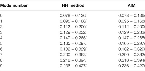
TABLE 1. First ten QNFs of the Klein-Gordon field produced by the HH method and by the AIM. We take r₊ = 70 and m = 1/10.

In Figure 1 we plot the real part and the imaginary part of the first ten QNFs for the Klein-Gordon field of mass m = 1/10 propagating in the 2D black hole (2) with radius of the horizon equal to r₊ = 70. We notice that the graph Im(ω) vs Re(ω) shows a linear relation between the imaginary part and the real part of the QNFs for the Klein-Gordon field as we change the mode number. We notice that in Figure 1 appear twenty points, but we consider as equivalent the QNFs with the same imaginary part, that is, we find two QNFs with the same imaginary part, but the real part of the first is the negative of the real part of the second.

FIGURE 1

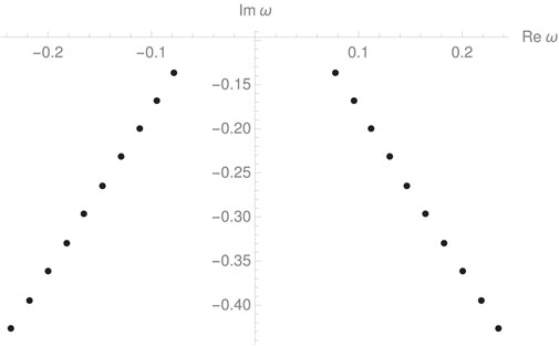
FIGURE 1. First ten QNFs of the Klein-Gordon field with mass m = 1/10 propagating in the 2D black hole (2) of radius r₊ = 70.

We notice that in the Figures of this paper (except for Figures 1, 6) we label the modes of the field as follows: n = 0, red circle; n = 1, blue square; n = 2, black diamond; n = 3, green triangle; n = 4, inverted magenta triangle.

For r₊ = 70, in Figures 2, 3 we present the variation of the imaginary part and the real part of the first five QNFs when we modify the mass of the Klein-Gordon field. In these figures we observe that the imaginary part and the real part of the QNFs change in a linear way as the mass varies. In Figures 2, 3 we observe that the imaginary part decreases, whereas the real part increases as the mass of the field increases, thus the QNMs of the Klein-Gordon decay faster and make more oscillations per time unit as the mass of the Klein-Gordon field increases.

FIGURE 2

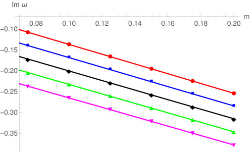
FIGURE 2. For the first five QNFs of the Klein-Gordon field we show how the imaginary part depends on the mass of the field. We consider a 2D black hole (2) of radius r₊ = 70.

FIGURE 3

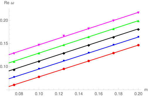
FIGURE 3. For the first five QNFs of the Klein-Gordon field we show how the real part depends on the mass of the field. We consider a 2D black hole (2) of radius r₊ = 70.

Furthermore, in Figures 2, 3 we show the plots of the linear fits given in Table 2. From the linear fits of Table 2 we see that for the plots Im(ω) vs. m the absolute value of the slope decreases as the mode number increases. For the plots Re(ω) vs. m we notice that the slope increases as the mode number increases. In both cases the change of slope with the mode number is small.

TABLE 2

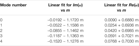
TABLE 2. For the Klein-Gordon field we give the linear fits for the points shown in Figures 2, 3. We take r₊ = 70.

In Figures 4, 5 we draw the behavior of the imaginary part and of the real part for the first five QNFs when the radius of the horizon varies and the mass of the Klein-Gordon field is m = 1/10. In these figures we see that the imaginary part increases, whereas the real part decreases as the radius of the black hole increases, thus, for a given mode the decay time increases and the oscillation frequency decreases as the horizon radius increases. In both figures we observe that the imaginary part and the real part of the fifth QNFs have the larger variations, whereas the imaginary part and the real part of the fundamental frequency show the smaller changes as the horizon radius increases.

FIGURE 4

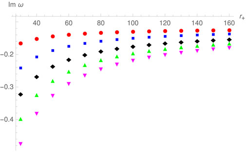
FIGURE 4. For the first five QNFs of the Klein-Gordon field we show how the imaginary part depends on the radius of the 2D black hole (2). We consider a Klein-Gordon field of mass m = 1/10.

FIGURE 5

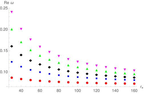
FIGURE 5. For the first five QNFs of the Klein-Gordon field we show how the real part depends on the radius of the 2D black hole (2). We consider a Klein-Gordon field of mass m = 1/10.

In Figures 4, 5 we also notice that the QNFs of the Klein-Gordon field in the 2D black hole (2) are more compactly distributed in the ω plane for bigger values of the horizon radius.

3.2 Numerical Results for the Dirac Field

For the Dirac field propagating in the 2D black hole (2) we find that, for the first ten modes, the two methods produce QNFs that agree to three decimal places. This fact is observed in Table 3 for a specific configuration (see Supplementary Appendix A for some numerical results with more decimal places). Furthermore, both methods yield QNFs with negative imaginary part, hence the QNMs of the Dirac field are stable in the 2D black hole (2).

TABLE 3

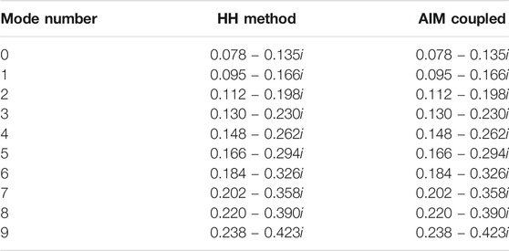
TABLE 3. First ten QNFs of the Dirac field produced by the HH method and by the AIM for coupled systems of first order differential equations. We take r₊ = 70 and m = 1/10.

Taking as a basis the HH method, for r₊ = 70 and m = 1/10, in Table 4 we observe that the QNFs produced by the effective potentials V₁ and V₂ of Eq. 38 are equal. Also, see the end of Supplementary Appendix B for another argument pointing out that these effective potentials generate the same QNFs. At present time we only have evidence that the effective potentials of Eq. 38 produce the same spectrum of QNF in the example studied in this work, but we think it would be convenient to show a more general result or find a case where they produce a different spectrum of QNF.

TABLE 4

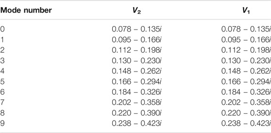
TABLE 4. We show the QNFs of the Dirac field produced by the effective potentials V₁ and V₂. We get these values for the QNFs using the HH method. We take r₊ = 70 and m = 1/10.

For the Dirac field, in Figures 6–9 and Supplementary Appendix Figure S1 we observe that the behavior of its QNFs is similar to that previously obtained for the QNFs of the Klein-Gordon field, hence we describe briefly the results for the Dirac field.

• For the QNFs of the Dirac field, in Figure 6 we see that the relation between the imaginary part and the real part of the QNFs is linear as we change the mode number, in a similar way to the QNFs of the Klein-Gordon field.

• In Figures 7, 8 we observe that the imaginary part and the real part of the QNFs for the Dirac field change in a linear way when we modify the value of the field’s mass. The linear fits of the data given in Figures 7, 8 are written in Table 5. In a similar way to the QNFs of the Klein-Gordon field we see that the imaginary part of the QNFs decreases as the field’s mass increases, whereas the real part of the QNFs increases as the field’s mass increases. As for the Klein-Gordon field, for the plots Im(ω) vs. m the absolute value of the slope decreases as the mode number increases. For the plots Re(ω) vs. m we find that the slope increases as the mode number increases. We also see that in both cases, the changes of the slope with the mode number are small.

• When we change the radius of the horizon, in Figure 9 and Supplementary Appendix Figure S1 we notice that for the QNFs of the Dirac field the imaginary part increases as the horizon radius increases, while the real part decreases as the horizon radius increases. These behaviors are similar to those for the QNFs of the Klein-Gordon field.

FIGURE 6

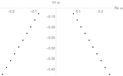
FIGURE 6. First ten QNFs of the Dirac field with mass m = 1/10 propagating in the 2D black hole (2) of radius r₊ = 70.

FIGURE 7

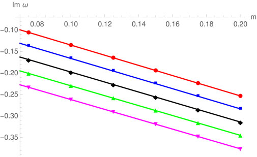
FIGURE 7. For the first five QNFs of the Dirac field we show how the imaginary part depends on the mass of the field. We consider a 2D black hole (2) of radius r₊ = 70.

FIGURE 8

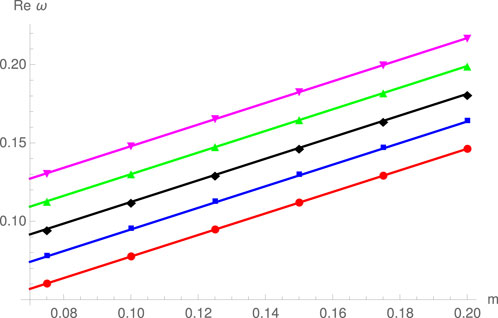
FIGURE 8. For the first five QNFs of the Dirac field we show how the real part depends on the mass of the field. We consider a 2D black hole (2) of radius r₊ = 70.

FIGURE 9

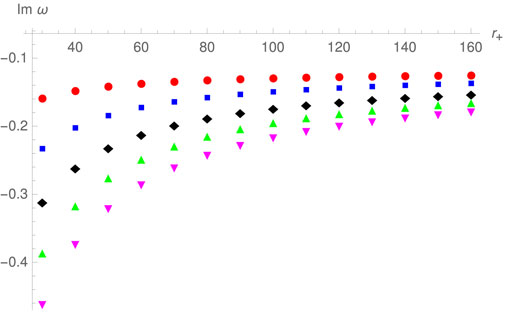
FIGURE 9. For the first five QNFs of the Dirac field we show how the imaginary part depends on the radius of the 2D black hole (2). We consider a Dirac field of mass m = 1/10.

TABLE 5

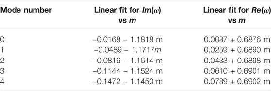
TABLE 5. For the Dirac field we give the linear fits for the points shown in Figures 7, 8. We take r₊ = 70.

As for the Klein-Gordon field, we also note that the QNFs of the Dirac field are more compactly distributed in the complex ω plane when the horizon radius is bigger.

4 Discussion

As far as we know, the AIM for coupled systems of first order differential equations has not previously used to calculate the QNFs of black holes. We find that the AIM for coupled systems of first order equations yields QNFs of the Dirac field in agreement with those that produces the HH method (see also Supplementary Appendices C, D). We believe that this method is appropriate for computing the QNFs of the Dirac field, since in many spacetimes its equation of motion simplifies to a coupled system of first order differential equations (Gibbons and Steif, 1993; Cotăescu, 1998; Lopez-Ortega, 2009), and in general the proposed method may be helpful to compute the QNFs of classical fields whose equations of motion simplify to a pair of coupled first order differential equations. Also this method for calculating the QNFs of the Dirac field may be useful to verify the results that are obtained with other numerical procedures. We notice that in Supplementary Appendix D, taking as a basis the improved formulation of the AIM for second order differential equations (Cho et al., 2010; Cho et al., 2012), we present an improved formulation of the AIM for coupled systems of first order differential equations.

For the two fields propagating in the asymptotically adS 2D black hole (2), we find that the HH method and the AIM produce the same values for their first ten QNFs (see also Supplementary Appendices C, D). Furthermore, in the numerical results we obtain QNFs with negative imaginary part, therefore the asymptotically adS 2D black hole (2) is stable under the Klein-Gordon and Dirac perturbations. A relevant fact is that its QNFs are complex, in contrast to other asymptotically adS 2D black hole in which purely imaginary QNFs are found (Cordero et al., 2012). As discussed in Section 3.1 and Section 3.2, in the numerical results we observe that the QNFs of the Klein-Gordon and Dirac fields behave in a similar way as we change the field’s mass or the radius of the horizon. As the mass increases, both fields decay faster and the oscillation frequencies increase. Furthermore, as the radius of the horizon increases the decay time increases, whereas the oscillation frequency decreases.

From the values presented in Tables 1, 3 we see that the QNFs of the Klein-Gordon and Dirac fields are similar, even though one field is bosonic and the other field is fermionic. Furthermore, in Supplementary Appendix Table S3 we display the numerical values of the QNFs for the Klein-Gordon and Dirac fields propagating in the 2D black holes (2) with radii r₊ = 30 and r₊ = 150. In this table we observe that for r₊ = 150 the QNFs of the two fields are essentially identical, also we note that for r₊ = 30 their QNFs are similar but they show more differences than the frequencies of the 2D black holes with radii r₊ = 70 and r₊ = 150. We also notice that for r₊ = 30 the fundamental QNFs are closer in value than the tenth QNFs. Thus the numerical results show that when the horizon radius increases the QNFs of the two fields are more similar. From the viewpoint of the Schrödinger type equations, these results are intriguing, because the analysis of the problem shows that for the two fields their effective potentials are very different. We also note that the effective potentials for the Dirac field fulfill.

$V_l=V_{KG}\mp \frac{i\omega }{2}\frac{df}{dr}-\frac{f}{4}\frac{d^{2}f}{d{r}^2}+\frac{1}{16}{\left(\frac{df}{dr}\right)}^2.(60)$

Although these differences, for some values of the physical parameters, the effective potentials V_l, V_KG produce almost isospectral QNFs in the asymptotically adS 2D black hole (2). Furthermore, as we previously mentioned, the QNFs of the effective potentials V_l, V_KG behave in a similar way when we change the physical parameters. Thus our numerical results indicate that for the 2D black hole (2) the last terms in the right hand side of the Eq. 60 have a small contribution to the value of the QNFs for the Dirac field. To start understanding this fact we notice the following facts. Near the horizon the last three terms in the Eq. 60 only produce a shift in the effective frequency that appears in the Schrödinger type equations, from ω for the Klein-Gordon field to (ω ± iκ/2) for the Dirac field. Therefore, near the horizon, for the Klein-Gordon field we get the radial solutions (9) whereas for the Dirac field we obtain the solutions (40). This fact does not prevent us from choosing the relevant solution for the QNMs. As r → ∞, the last three terms in Eq. 60 produce that the dominant behavior of the effective potentials change from V_KG ∼ a²r²m² for the Klein-Gordon field to V_l ∼ a²r²(m² − a²/4) for the Dirac field, that is, only produce a shift in the value of the mass. In our case this change does not prevent us from choosing the appropriate solution that satisfies the boundary condition of the QNMs at the asymptotic region.

Data Availability Statement

The original contributions presented in the study are included in the article/Supplementary Material, further inquiries can be directed to the corresponding author.

Author Contributions

All authors listed have made a substantial, direct, and intellectual contribution to the work and approved it for publication.

Funding

This work was supported by CONACYT México, SNI México, EDI-IPN, COFAA-IPN, and Research Project IPN SIP 20210485.

Conflict of Interest

The authors declare that the research was conducted in the absence of any commercial or financial relationships that could be construed as a potential conflict of interest.

Publisher’s Note

All claims expressed in this article are solely those of the authors and do not necessarily represent those of their affiliated organizations, or those of the publisher, the editors and the reviewers. Any product that may be evaluated in this article, or claim that may be made by its manufacturer, is not guaranteed or endorsed by the publisher.

Supplementary Material

The Supplementary Material for this article can be found online at: https://www.frontiersin.org/articles/10.3389/fspas.2021.713422/full#supplementary-material

Footnotes

¹In this work, for Eq. 26 we use the name of quantization condition (Ciftci et al., 2003), but notice that here we explore the classical propagation of the Klein-Gordon and Dirac fields. In the context of this paper a more appropriate name for Eq. 26 could be discretization condition or termination condition.

²We note that the effective potentials (36) are supersymmetric partners. The superpotential is equal to $W=-m\sqrt{f}$ (Cooper et al., 1995; López-Ortega and Vega-Acevedo, 2011).

³In this work our convention for the QNFs is ω = Re(ω) + iIm(ω). Therefore a complex frequency with negative imaginary part is related with a wave that decays in time (see the time dependence in the Eq. 5).

References

Avis, S. J., Isham, C. J., and Storey, D. (1978). Quantum Field Theory in Anti-de Sitter Space-Time. Phys. Rev. D 18, 3565–3576. doi:10.1103/PhysRevD.18.3565

CrossRef Full Text | Google Scholar

Balasubramanian, K., and McGreevy, J. (2009). An Analytic Lifshitz Black Hole. Phys. Rev. D 80, 104039. [arXiv:0909.0263 [hep-th]]. doi:10.1103/physrevd.80.104039

CrossRef Full Text | Google Scholar

Becar, R., Lepe, S., and Saavedra, J. (2010). Decay of Dirac Fields in the Backgrounds of Dilatonic Black Holes. Int. J. Mod. Phys. A. 25, 1713–1723. doi:10.1142/S0217751X10048275

CrossRef Full Text | Google Scholar

Becar, R., Lepe, S., and Saavedra, J. (2007). Quasinormal Modes and Stability Criterion of Dilatonic Black Holes In1+1and4+1dimensions. Phys. Rev. D 75, 084021. [arXiv:gr-qc/0701099]. doi:10.1103/PhysRevD.75.084021

CrossRef Full Text | Google Scholar

Berti, E., Cardoso, V., and Starinets, A. O. (2009). Quasinormal Modes of Black Holes and Black Branes. Class. Quan. Grav. 26, 163001. [gr-qc]. doi:10.1088/0264-9381/26/16/163001

CrossRef Full Text | Google Scholar

Bhattacharjee, S., Sarkar, S., and Bhattacharyya, A. (2021). Scalar Perturbations of Black Holes in Jackiw-Teitelboim Gravity. Phys. Rev. D 103 (no.2), 024008. arXiv:2011.08179 [gr-qc]. doi:10.1103/PhysRevD.103.024008

CrossRef Full Text | Google Scholar

Boyce, W. E., and Di Prima, R. C. (2008). Elementary Differential Equations. John Wiley and Sons, United States of America.

Breitenlohner, P., and Freedman, D. Z. (1982). Positive Energy in Anti-de Sitter Backgrounds and Gauged Extended Supergravity. Phys. Lett. B 115, 197–201. doi:10.1016/0370-2693(82)90643-8

CrossRef Full Text | Google Scholar

Burgess, C. P., and Lütken, C. A. (1985). Propagators and Effective Potentials in Anti-de Sitter Space. Phys. Lett. B 153, 137–141. doi:10.1016/0370-2693(85)91415-7

CrossRef Full Text | Google Scholar

Catalán, M., Cisternas, E., Vásquez, P. A., and Vasquez, Y. (2014). Dirac Quasinormal Modes for a 4-dimensional Lifshitz Black Hole. Eur. Phys. J. C 74, 2813. [arXiv:1312.6451 [gr-qc]]. doi:10.1140/epjc/s10052-014-2813-7

CrossRef Full Text | Google Scholar

Chan, J. S. F., and Mann, R. B. (1997). Scalar Wave Falloff in Asymptotically Anti-de Sitter Backgrounds. Phys. Rev. D 55, 7546–7562. [arXiv:gr-qc/9612026 [gr-qc]]. doi:10.1103/PhysRevD.55.7546

CrossRef Full Text | Google Scholar

Chan, J. S. F., and Mann, R. B. (1999). Scalar Wave Falloff in Topological Black Hole Backgrounds. Phys. Rev. D 59, 064025. doi:10.1103/PhysRevD.59.064025

CrossRef Full Text | Google Scholar

Chandrasekhar, S. (1992). The Mathematical Theory of Black Holes. Oxford: Oxford University Press.

Cho, H., Cornell, A., Doukas, J., Huang, T., and Naylor, W. (2012). A New Approach to Black Hole Quasinormal Modes: A Review of the Asymptotic Iteration Method. Adv. Math. Phys. 2012, 281705. [arXiv:1111.5024 [gr-qc]]. doi:10.1155/2012/281705

CrossRef Full Text | Google Scholar

Cho, H. T. (2003). Dirac Quasinormal Modes in Schwarzschild Black Hole Space-Times. Phys. Rev. D 68, 024003. [arXiv:gr-qc/0303078 [gr-qc]]. doi:10.1103/PhysRevD.68.024003

CrossRef Full Text | Google Scholar

Cho, H. T., Cornell, A. S., Doukas, J., and Naylor, W. (2010). Black Hole Quasinormal Modes Using the Asymptotic Iteration Method. Class. Quan. Grav. 27, 155004. [gr-qc]. doi:10.1088/0264-9381/27/15/155004

CrossRef Full Text | Google Scholar

Ciftci, H., Hall, R. L., and Saad, N. (2003). Asymptotic Iteration Method for Eigenvalue Problems. J. Phys. A: Math. Gen. 36, 11807–11816. doi:10.1088/0305-4470/36/47/008

CrossRef Full Text | Google Scholar

Ciftci, H., Hall, R. L., and Saad, N. (2005). Iterative Solutions to the Dirac Equation. Phys. Rev. A. 72, 022101. doi:10.1103/PhysRevA.72.022101

CrossRef Full Text | Google Scholar

Cooper, F., Khare, A., and Sukhatme, U. (1995). Supersymmetry and Quantum Mechanics. Phys. Rep. 251, 267–385. [arXiv:hep-[hep-th]]. doi:10.1016/0370-1573(94)00080-M

CrossRef Full Text | Google Scholar

Cordero, R., López-Ortega, A., and Vega-Acevedo, I. (2012). Quasinormal Frequencies of Asymptotically Anti-de Sitter Black Holes in Two Dimensions. Gen. Relativ Gravit. 44, 917–940. arXiv:1201.3605 [gr-qc]. doi:10.1007/s10714-011-1316-1

CrossRef Full Text | Google Scholar

Cotăescu, I. I. (1998). The Dirac Particle on De Sitter Background. Mod. Phys. Lett. A. 13, 2991–2997. [arXiv:gr-qc/9808030 [gr-qc]]. doi:10.1142/S021773239800317X

CrossRef Full Text | Google Scholar

Dasgupta, A. (1999). Emission of Fermions from BTZ Black Holes. Phys. Lett. B 445, 279–286. [arXiv:hep-th/9808086 [hep-th]]. doi:10.1016/S0370-2693(98)01492-0

CrossRef Full Text | Google Scholar

Destounis, K. (2019). Charged Fermions and strong Cosmic Censorship. Phys. Lett. B 795, 211–219. arXiv:1811.10629 [gr-qc]. doi:10.1016/j.physletb.2019.06.015

CrossRef Full Text | Google Scholar

Estrada-Jiménez, S., Gómez-Díaz, J. R., and López-Ortega, A. (2013). Quasinormal Modes of a Two-Dimensional Black Hole. Gen. Relativ Gravit. 45, 2239–2250. arXiv:1308.5943 [gr-qc]. doi:10.1007/s10714-013-1582-1

CrossRef Full Text | Google Scholar

Finster, F., Smoller, J., and Yau, S.-T. (2000). Non-existence of Time-Periodic Solutions of the Dirac Equation in a Reissner-Nordström Black Hole Background. J. Math. Phys. 41, 2173–2194. [arXiv:gr-qc/9805050 [gr-qc]]. doi:10.1063/1.533234

CrossRef Full Text | Google Scholar

Giacomini, A., Giribet, G., Leston, M., Oliva, J., and Ray, S. (2012). Scalar Field Perturbations in Asymptotically Lifshitz Black Holes. Phys. Rev. D 85, 124001. [arXiv: 1203.0582 [hep-th]]. doi:10.1103/physrevd.85.124001

CrossRef Full Text | Google Scholar

Giammatteo, M., and Jing, J. (2005). Dirac Quasinormal Frequencies in Schwarzschild-AdS Space-Time. Phys. Rev. D 71, 024007. [arXiv:gr-qc/0403030 [gr-qc]]. doi:10.1103/PhysRevD.71.024007

CrossRef Full Text | Google Scholar

Gibbons, G. W., and Steif, A. R. (1993). Anomalous Fermion Production in Gravitational Collapse. Phys. Lett. B 314, 13–20. [arXiv:gr-qc/9305018 [gr-qc]]. doi:10.1016/0370-2693(93)91315-E

CrossRef Full Text | Google Scholar

Grumiller, D., Kummer, W., and Vassilevich, D. V. (2002). Dilaton Gravity in Two Dimensions. Phys. Rep. 369, 327–430. doi:10.1016/S0370-1573(02)00267-3

CrossRef Full Text | Google Scholar

Grumiller, D., and Meyer, R. (2006). Ramifications of Lineland. Turk. J. Phys. 30, 349–378. [hep-th/0604049].

Hod, S. (1998). Bohr's Correspondence Principle and the Area Spectrum of Quantum Black Holes. Phys. Rev. Lett. 81, 4293–4296. [arXiv:gr-qc/9812002 [gr-qc]]. doi:10.1103/PhysRevLett.81.4293

CrossRef Full Text | Google Scholar

Horowitz, G. T., and Hubeny, V. E. (2000). Quasinormal Modes of AdS Black Holes and the Approach to Thermal Equilibrium Phys. Rev. D 62, 024027. [hep-th/9909056]. doi:10.1103/PhysRevD.62.024027

CrossRef Full Text

Jing, J. I. (2005). Quasinormal Modes of Dirac Field Perturbation in Schwarzschild-anti-de Sitter Black Hole [arXiv:gr-qc/0502010 [gr-qc]]. Available at https://arxiv.org/abs/gr-qc/0502010 (Accessed August 5, 2021).

Jusufi, K., Sakallı, I., and Ovgün, A. (2018). Quasinormal Modes of Stringy Black Holes. Gen. Rel. Grav. 50 (no.1), 10. [arXiv:1709.03923 [gr-qc]]. doi:10.1007/s10714-017-2330-8

CrossRef Full Text | Google Scholar

Kettner, J., Kunstatter, G., and Medved, A. J. M. (2004). Quasinormal Modes for Single Horizon Black Holes in Generic 2D Dilaton Gravity. Class. Quan. Grav. 21, 5317–5332. doi:10.1088/0264-9381/21/23/002

CrossRef Full Text | Google Scholar

Kokkotas, K. D., and Schmidt, B. G. (1999). Quasi-Normal Modes of Stars and Black Holes. Living Rev. Relativ. 2, 2. [arXiv:gr-qc/9909058]. doi:10.12942/lrr-1999-2

PubMed Abstract | CrossRef Full Text | Google Scholar

Konoplya, R. A., and Zhidenko, A. (2011). Quasinormal Modes of Black Holes: From Astrophysics to String Theory. Rev. Mod. Phys. 83, 793–836. arXiv:1102.4014 [gr-qc]]. doi:10.1103/RevModPhys.83.793

CrossRef Full Text | Google Scholar

Kwon, Y., and Nam, S. (2010). Area Spectra of the Rotating BTZ Black Hole from Quasinormal Modes. Class. Quan. Grav. 27, 125007. [hep-th]]. doi:10.1088/0264-9381/27/12/125007

CrossRef Full Text | Google Scholar

Lemos, J. P. S., and Sá, P. M. (1994). Black Holes of a General Two-Dimensional Dilaton Gravity Theory. Phys. Rev. 49, 2897. doi:10.1103/PhysRevD.49.2897

CrossRef Full Text | Google Scholar

Lemos, J. P. S. (1995). Two-dimensional Black Holes and Planar General Relativity. Class. Quan. Grav. 12, 1081–1086. [gr-qc]]. doi:10.1088/0264-9381/12/4/014

CrossRef Full Text | Google Scholar

Li, X.-z., Hao, J.-g., and Liu, D.-j. (2001). Quasinormal Modes of Stringy Black Holes. Phys. Lett. B 507, 312–316. [gr-qc/0205007]. doi:10.1016/S0370-2693(01)00437-3

CrossRef Full Text | Google Scholar

Lopez-Ortega, A. (2010). Quasinormal Frequencies of the Dirac Field in the Massless Topological Black Hole. Rev. Mex. Fis. 56, 44–53. [arXiv:1006.4906 [gr-qc]].

Lopez-Ortega, A. (2014). Quasinormal Frequencies of the Dirac Field in a D-dimensional Lifshitz Black Hole. Rev. Mex. Fis. 60 (5), 357𠈓365. [arXiv:1407.0966 [gr-qc]].

López-ortega, A. (2012). Classical Stability of Black Holes under Massless Dirac Perturbations. Int. J. Mod. Phys. D 21, 1250092. [arXiv:1211.1801 [gr-qc]]. doi:10.1142/S0218271812500927

CrossRef Full Text | Google Scholar

López-Ortega, A. (2004). Dirac Fields in 3D de Sitter Spacetime. Gen. Relativity Gravitation 36, 1299–1319. doi:10.1023/B:GERG.0000022389.05399.6d

CrossRef Full Text | Google Scholar

López-Ortega, A. (2014). Electromagnetic Quasinormal Modes of an Asymptotically Lifshitz Black Hole. Gen. Relativ Gravit. 46, 1756. [arXiv:1406.0126 [gr-qc]]. doi:10.1007/s10714-014-1756-5

CrossRef Full Text | Google Scholar

López-ortega, A. (2011). Entropy Spectra of Single Horizon Black Holes in Two Dimensions. Int. J. Mod. Phys. D 20, 2525–2542. [arXiv:1112.6211 [gr-qc]]. doi:10.1142/S0218271811020524

CrossRef Full Text | Google Scholar

López-Ortega, A. (2010). Entropy Spectrum of the D-Dimensional Massless Topological Black Hole. Gen. Relativ Gravit. 42, 2939–2945. [arXiv:1006.5039 [gr-qc]]. doi:10.1007/s10714-010-1049-6

CrossRef Full Text | Google Scholar

Lopez-Ortega, A. (2009). The Dirac Equation in D-dimensional Spherically Symmetric Spacetimes. Lat. Am. J. Phys. Educ. 3, 578. [arXiv:0906.2754 [gr-qc]]. doi:10.1109/te.2009.2035424

CrossRef Full Text | Google Scholar

López-ortega, A. (2009). Quasinormal Modes and Stability of a Five-Dimensional Dilatonic Black Hole. Int. J. Mod. Phys. D 18, 1441–1459. [arXiv:0905.0073 [gr-qc]]. doi:10.1142/S0218271809015199

CrossRef Full Text | Google Scholar

López-Ortega, A., and Vega-Acevedo, I. (2011). Quasinormal Frequencies of Asymptotically Flat Two-Dimensional Black Holes. Gen. Relativ Gravit. 43, 2631–2647. arXiv:1105.2802 [gr-qc]]. doi:10.1007/s10714-011-1185-7

CrossRef Full Text | Google Scholar

Maggiore, M. (2008). Physical Interpretation of the Spectrum of Black Hole Quasinormal Modes. Phys. Rev. Lett. 100, 141301. [arXiv:0711.3145 [gr-qc]]. doi:10.1103/PhysRevLett.100.141301

PubMed Abstract | CrossRef Full Text | Google Scholar

Mirbabayi, M. (2020). The Quasinormal Modes of Quasinormal Modes. J. Cosmol. Astropart. Phys. 2020, 052. [arXiv:1807.04843 [gr-qc]]. doi:10.1088/1475-7516/2020/01/052

CrossRef Full Text | Google Scholar

Myung, Y. S., and Moon, T. (2012). Quasinormal Frequencies and Thermodynamic Quantities for the Lifshitz Black Holes. Phys. Rev. D 86, 024006. arXiv:1204.2116 [hep-th]]. doi:10.1103/PhysRevD.86.024006

CrossRef Full Text | Google Scholar

Newman, E., and Penrose, R. (1962). An Approach to Gravitational Radiation by a Method of Spin Coefficients. J. Math. Phys. 3, 556. doi:10.1063/1.1724257

CrossRef Full Text | Google Scholar

Sakalli, İ., and Tokgöz Hyusein, G. (2021). Quasinormal Modes of Charged Fermions in Linear Dilaton Black Hole Spacetime: Exact Frequencies. Turk. J. Phys. 45 (1), 43–58. [arXiv:2102.03595 [hep-th]]. doi:10.3906/fiz-2012-6

CrossRef Full Text | Google Scholar

Sakallı, İ., Jusufi, K., and Övgün, A. (2018). Analytical Solutions in a Cosmic String Born–Infeld-Dilaton Black Hole Geometry: Quasinormal Modes and Quantization. Gen. Rel. Grav. 50 (no.10), 125. [arXiv:1803.10583 [gr-qc]]. doi:10.1007/s10714-018-2455-4

CrossRef Full Text | Google Scholar

Kanzi, S., and Sakallı, İ., (2021). Greybody Radiation and Quasinormal Modes of Kerr-like Black Hole in Bumblebee Gravity Model. The Eur. Phys. J. C. 81, 501. doi:10.1140/epjc/s10052-021-09299-y

CrossRef Full Text | Google Scholar

Stetsko, M. M. (2017). Fermionic Quasinormal Modes for Two-Dimensional Hořava-Lifshitz Black Holes. Eur. Phys. J. C 77, 416 [arXiv:1612.09172 [hep-th]]. doi:10.1140/epjc/s10052-017-4983-6

CrossRef Full Text | Google Scholar

Wei, S., and Liu, Y. (2009). Area Spectrum of the Large AdS Black Hole from Quasinormal Modes [arXiv:0906.0908 [hep-th]]. Available at https://arxiv.org/abs/0906.0908 (Accessed August 5, 2021).

Zelnikov, A. (2008). Non-minimal scalar fields in 2D de Sitter and dilaton black holes. J. High Energ. Phys. 2008, 010. [hep-th]]. doi:10.1088/1126-6708/2008/07/010

CrossRef Full Text | Google Scholar