 Shishir Priyadarshi
 Jian Yang
 Weiqin Sun
- 1Department of Earth and Space Sciences, Southern University of Science and Technology, Shenzhen, China
- 2School of Atmospheric Sciences, Sun Yat-Sen University, Zhuhai, China
Interaction between Earth’s magnetotail and its inner magnetosphere plays an important role in the transport of mass and energy in the ionosphere–magnetosphere coupled system. A number of first-principles models are devoted to understanding the associated dynamics. However, running these models, including both magnetohydrodynamic models and kinetic drift models, can be computationally expensive when self-consistency and high spatial resolution are required. In this study, we exploit an approach of building a parallel statistical model, based on the long short-term memory (LSTM) type of recurrent neural network, to forecast the results of a first-principles model, called the Rice Convection Model (RCM). The RCM is used to simulate the transient injection events, in which the flux-tube entropy parameter, dawn-to-dusk electric field component, and cumulative magnetic flux transport are calculated in the central plasma sheet. These key parameters are then used as initial inputs for training the LSTM. Using the trained LSTM multivariate parameters, we are able to forecast the plasma sheet parameters beyond the training time for several tens of minutes that are found to be consistent with the subsequent RCM simulation results. Our tests indicate that the recurrent neural network technique can be efficiently used for forecasting numerical simulations of magnetospheric models. The potential to apply this approach to other models is also discussed.
Key Points
1. Simulation results of the RCM (a physics-based model) are used as inputs for training the LSTM-based RNN model for the forecast of the longer duration.
2. The approach is applied to multiple simulations of idealized low-entropy bubble injection events.
3. There is a great consistency between the LSTM-based forecast and the RCM results beyond the training time.
Introduction
Data in Earth’s magnetosphere are less available than in other regions (e.g., the ionosphere, the lower atmosphere, and ground-based observations of the upper atmosphere) based on their spatial and temporal continuity. Therefore, for developing a machine learning model, the output from a physics-based model can serve as an input asset due to the continuous temporal/spatial availability of their outputs. Besides, it is always good to train a machine learning model using a known and stable environment (e.g., an existing model in our case). This allows the machine learning model to learn the time series quickly and understand the underlying relationship among the time series of several physics-based models’ output parameters.
Previous works have adapted artificial neural networks (ANNs) to study space weather. For example, Koon and Gorney (1991) used Los Alamos National Laboratory (LANL) particle data for the prediction of daily averaged electrons with an energy of >3 MeV. Stringer et al. (1996) used ANNs on GOES-7 data for nowcasting 1-h geosynchronous orbit electron flux at energies of 3–5 MeV. The work of Stringer et al. (1996) was extended to one-day forecast by Ukhorskiy et al. (2004) and Kitamura et al. (2011). A relativistic electron flux at a geosynchronous orbit––forecasting neural network (NN) model was developed by Ling et al. (2010). They used historical electron flux values and daily summed values of the planetary Kp index over two neurons, and their neural network model showed better prediction than the Relativistic Electron Forecast Model (REFM) developed by Baker et al. (1990). The NNs were also used on solar wind inputs to predict geosynchronous electron distributions over wide energy ranges and for a number of time resolutions (Shin et al., 2016; Wei et al., 2018). Wiltberger et al. (2017) used machine learning analysis of the magnetosphere–ionosphere field-aligned current (FAC) patterns and found out that the ratio of Region 1 (R1) to Region 2 (R2) current decreases as the simulation resolution increases. This application of machine learning to the FAC analysis helped establish a better agreement in the simulation results than the Weimer 2005 model (Weimer, 2005). They used a Python-based open source Scikit-Learn algorithm package developed by Pedregosa et al. (2011), which allows supervised and unsupervised machine learning algorithms. Other space weather–related research that uses machine learning techniques has also been reviewed by Camporeale (2019). Recently, Pires de Lima et al. (2020) used a convolution neural network (CNN) to build a predictive model for the MeV electrons inside Earth’s outer radiation belt. The model of Pires de Lima and Lin, known as PreMevE 2.0, is a supervised machine learning model, and it can forecast the onset of MeV electron events in 2 days. The Pires de Lima and Lin model uses electron data observed by the particle instruments of RBSP spacecraft, one geo-satellite of the Los Alamos National Laboratory (LANL), and one NOAA Polar Operational Environmental Satellite (POES) for the time duration from February 2013 to August 2016.
A recurrent neural network (RNN) is a state-of-the-art approach that combines several algorithms to enable them to learn the time series of datasets (Connor et al., 1994; Graves et al., 2013). However, due to the limited memory, the error becomes larger when the longer (e.g., more than a hundred data time steps) training datasets in the RNN are used. The wait function, which is a statistical and analytical tool used to characterize input parameters’ influence on the prediction, also becomes erroneous with time (Graves and Schmidhuber, 2005). On the other hand, a long short-term memory (LSTM)–based neural network is a kind of recurrent neural network which can memorize time series datasets with very long duration and also forget them if some part of the dataset is not necessary. The LSTM uses the sigmoid function for keeping things in its memory and TANH functions if the LSTM states decide to remove the memory after finding it useless for future time series forecasting (Eck and Schmidhuber, 2002). The sigmoid functions are best for modeling the physical processes that start with the small beginnings but attain a high saturated value over time as the specific models often fail to reproduce such processes (Gers et al., 2000).
LSTM has already been used in robot control, speech recognition, rhythm learning, music composition, grammar learning, handwriting recognition, human language recognition, sign language translation, and many more scientific and nonscientific disciplines. The LSTM-based models can be made scientific by sensibly choosing the input datasets and the training and testing periods of time. To do this, one has to first think about what are the most suitable inputs and in what order they should be fed in the LSTM algorithm to bring satisfactory outputs. Once the inputs and the training/testing periods are defined, the final LSTM model can be fitted to the entire dataset. The magnetosphere is a region where only sparse numbers of in situ measurements exist so far. A machine learning model can prove them to be an asset to better understand, analyze, and forecast the evolution and dynamics of magnetosphere physics during different kinds of space weather events or simulations. First-principles models reflect purely physics-based laws, and such models are generally represented by mathematical equations. They can be effectively converted into a machine learning statistical model by creating a multivariate time series of the variables used in the mathematical equations of the parameters we are going to model.
The phenomenon we will study in this article is the earthward injection of plasma sheet bubbles. A plasma sheet bubble has a lower flux-tube entropy parameter, PV5/3, than its neighbors (Pontius and Wolf, 1990). Here, P is the plasma pressure and V = ∫ds/B is the flux-tube volume per unit magnetic flux. Dependent on their observational signatures, they are also called earthward flow channels or bursty bulk flows (BBFs) (Angelopoulos et al., 1992). They are found to be associated with enhanced energetic particle flux near the geosynchronous orbit (McIlwain 1972, 1974; Yang et al., 2010a, Yang et al., 2010b; 2011 and references therein). These earthward flows are associated with the dipolarized northward magnetic field Bz, and they also lead to pulses of the enhanced dawn-to-dusk electric field component Ey (Nakamura et al., 2002; Runov et al., 2009; Liu et al., 2013; Khotyaintsev et al., 2011; Birn et al., 2019). As a consequence, the magnetic flux transport is earthward with a positive Ey. Here, the cumulative magnetic flux transport (CMFT) is defined (Birn et al., 2019) as follows:
The Rice Convection Model (RCM) is a first-principles physics-based model of the inner magnetosphere and the plasma sheet which can simulate drifts of different isotropic particles using the many-fluid formalism (Toffoletto et al., 2003 and references therein). It has been widely used to simulate the bubble injections and flow channels associated with substorm activities (Zhang et al., 2008; Yang et al., 2011; Lemon et al., 2004). Although the computational speed has been greatly improved by using Message Passing Interface (MPI) parallel programming in the RCM and the coupled MHD code (Yang et al., 2019; Silin et al., 2013), it is still computation-heavy. On the other hand, LSTM-based RNN models learn from the time series and multivariate inputs, and the underlying relationship between different variables can make the LSTM learn the relative simultaneous changes in the different input variables with time and it boosts the LSTM forecast capabilities. Therefore, combining the RCM with the LSTM technique can be a nice attempt at converting a first-principles physics-based model into a statistical model that abides by scientific laws used in the RCM.
In the next section, we will discuss the methodology, the boundary condition in the RCM, and our RNN modeling approach. In the third section, we will validate RNN results by comparing them with the RCM outputs. A detailed error analysis is discussed in the “LSTM Forecast Error Analysis” section for all the three runs by dividing the entire simulation region into four sectors. The last section will conclude the presented study and discuss our future plans for developing the statistical model using the well-established magnetospheric models.
Methodology and Model Setup
Setup of RCM Simulations
In this study, we performed three different RCM runs. The initial conditions are set the same way as in Yang et al. (2011), in which the plasma distribution and the magnetic field configuration are specified according to empirical models driven by idealized solar wind parameters. In all the RCM runs used in this study, the solar wind condition is assumed to be steady; IMF Bz is −5 nT and Bx and By are assumed to be zero. The solar wind velocity Vx = −400 km/s, and the other components are assumed to be zero. The solar wind proton number density is 5 cm−3, and the solar dynamic pressure is 1.34 nPa. The IRI-90 (International Reference Ionosphere) empirical ionospheric model plus conductance enhancement due to the electron precipitation is used to calculate the ionospheric conductance. An ellipse is set in the equatorial plane as the outer boundary of the RCM simulation region. The total potential drop across the RCM boundary is set to 30 kV (Yang et al., 2015; Yang et al., 2016).
Boundary Conditions for a Single Bubble Injection
A bubble is launched from the tailward boundary centered at X = −18.0 Re and Y = 0 Re. The entropy parameter PV5/3 is uniformly reduced to 2% in 10 min between 23.5 and 0.5 h MLT. The magnetic local time noon 12 MLT corresponds to Φ = 0 radians; 18 MLT, 0 MLT, and 6 MLT correspond to Φ = π/2, π, and 1.5π radians, respectively. The boundary condition for the flux-tube content
Here,
Boundary Conditions for a Single Flow Channel
In this run, the depletion in PV5/3 is sustained until T = 59 min. The flow channel is centered at midnight with a width of 0.5 h in local time, that is, from ΦW = 11.75/12 π to ΦE = 12.25/12 π. The boundary condition for the flux-tube content
Boundary Conditions for Three Flow Channels
Out of the three flows, one flow is centered at midnight with a width of 0.5 h in local time, that is, from ΦW = 11.75/12 π to ΦE = 12.25/12 π, and the other two are at ΦW = 7/9 π to ΦE = 5/6 π and ΦW = 7/6 π to ΦE = 11/9 π. The flux-tube content
We run the RCM simulation for 60 min. Out of several output parameters, we have used the entropy parameter, dawn-to-dusk electric field component, and cumulative magnetic flux for the presented LSTM modeling of the three plasma sheet parameters. The 1-h RCM simulations output these parameters every minute.
LSTM–RNN–Based Modeling
We use Python’s Keras (https://keras.io/) deep learning library to prepare and fit the LSTM forecast based on the RCM’s outputs. To train the LSTM, 50 neurons are used in the first hidden layer and one neuron is used for the output layer. After several experiments, we found that 30 training epochs and 72 batch sizes are good enough for the internal state of our LSTM model. We have developed three independent LSTM models for PV5/3, Ey, and cumulative magnetic flux ϕ. We cannot model the magnetic field in the RCM-MHD code using LSTM, as for now, it is hard to include additional constraint to the LSTM to ensure the divergence-free nature of the magnetic field. On the other hand, it is challenging to include some additional constraints in the LSTM to make it satisfy the MHD force balance equation for Bz and Vx. Due to these issues, we decided to model only PV5/3, Ey, and ϕ. We use simulation time for indexing the time series data, and we use the multivariate LSTM to train the RCM boundary condition–dependent machine learning model about the time series and the underlying relationship of the different input parameters used in our algorithm. All RCM and LSTM variables in the following equations are in two dimensions (i.e., in X and Y coordinates, which are in Re units).
The above input datasets are the best combination of the input variables in terms of their order in the given function, as we get the minimal root mean square error (RMSE) and minimal training and test loss between the RCM and the LSTM for these input combinations. From the left to the right in the RHS of each equation, the weight of the variable gradually decreases.
Figure 1 shows the scheme of our LSTM model. This scheme demonstrates that we have 61 steps (0–60 min) of RCM simulation, out of which we use 0–30 min of simulation to train three independent multivariate time series LSTM models. Using these models, we forecast 31–60 min of the RCM simulation, and then we compare the LSTM forecast with the 31–60 min of RCM simulation during three different runs. If there is a good agreement between the LSTM forecast and the RCM simulation for 31–60 min of the solution time, we fit the same model for the entire data length of the time series, that is, from 0 to 60 min of solution time. Using this LSTM model, we have forecasted the entire series. As a final check after the model fitting, we see if the final LSTM forecast is ±10% (in our case) of the RCM simulation, in which case the LSTM forecast meets our expectations, and we can forecast the entire RCM runs’ data time series. Although the RCM simulation is in 2D (X and Y both are in the unit of Earth radii–Re) coordinates, we do not use the X and Y coordinates as an input parameter in our LSTM model. The LSTM model for the presented three parameters is represented by Eqs 4–6, and it is also presented as a scheme diagram in Figure 1. The order of input parameters for forecasting different inner magnetosphere and plasma sheet variables will be according to their modeling in Eqs 4–6.
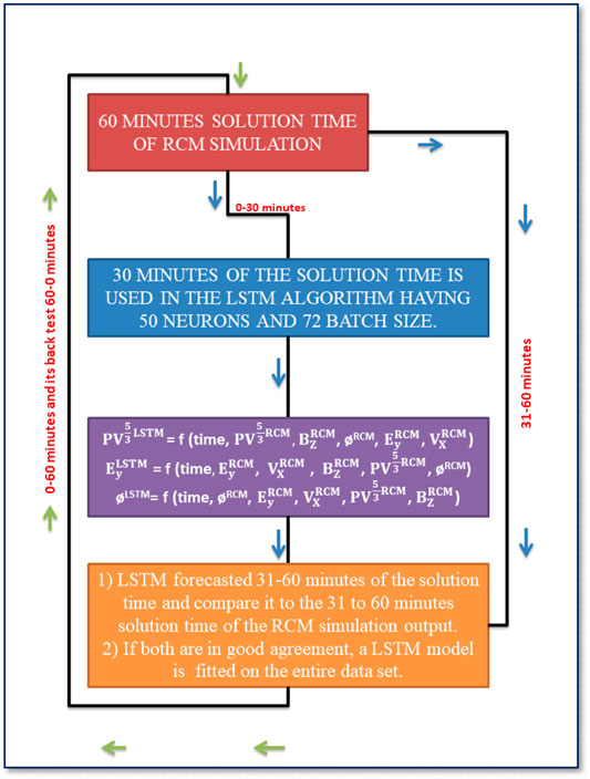
FIGURE 1. Scheme for RNN-based LSTM modeling of cumulative magnetic flux (CMFT) ϕ in Wb/Re; dawn-to-dusk electric field Ey in mV/m; and entropy parameter PV5/3 in nPa [Re/nT]5/3 using the first 0–30 min of the RCM simulation as inputs.
Model Validation
In this section, we will use an example of the single bubble run to demonstrate the consistency between the RCM simulation results and the LSTM forecast at a given location.
Figure 2 shows the RCM simulation results at T = 8 min of the single bubble event. Figure 2A shows a single low-entropy bubble centered at the midnight region of the plasma sheet. At the same time, Ey is significantly enhanced (Figure 2B), which is around 1 mV/m at the edge of the bubble, and it has a peak value of >2 mV/m inside the bubble. The northward component of the magnetic field Bz is enhanced to ∼20 nT (Figure 2C) at the leading head of the bubble, and the cumulative magnetic flux ϕ (Figure 2D) shows enhancement with respect to the surrounding background.
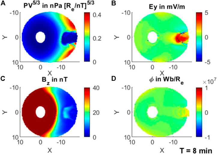
FIGURE 2. Single bubble run at T = 8 min; (A) entropy parameter PV5/3 in nPa [Re/nT]5/3; (B) dawn-to-dusk component of the electric field Ey in mV/m; (C) BZ in nT; and (D) cumulative magnetic flux transport ϕ in Wb/Re. X and Y are in Earth’s radii (Re) units. The Sun is to the left.
Figure 3 shows the RCM simulation of the same event at the solution time T = 30 min, where PV5/3 on the tailward boundary is already recovered to the value prior to the injection. PV5/3 increases tailward. The most significant enhancement is ϕ, and this enhancement is aligned with the direction of the launch of the bubble and its vicinity where the ϕ is increasing with time. In summary, this single bubble simulation shows features of typical injections, which can cause abrupt changes in the magnetotail parameters.
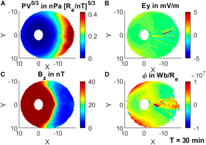
FIGURE 3. Single bubble run at T = 30 min; (A) entropy parameter PV5/3 in nPa [Re/nT]5/3; (B) dawn-to-dusk component of the electric field Ey in mV/m; (C) BZ in nT; and (D) cumulative magnetic flux transport ϕ in Wb/Re.
Using Eqs 4, 5 and 6, we have developed three independent LSTM-based RNN models for ϕ, Ey, and PV5/3. To perform this action, we trained our LSTM RNN model with the first 30 min of the RCM simulation. The trained LSTM is used to reproduce the 60-min single bubble injection. Now, we will compare the entire 60 min between the RCM and the LSTM results. Figure 4 shows the comparison of the single bubble RCM simulation (blue line) to the LSTM forecast (orange line) for the single point at X = −9.9 Re and Y = −1.1 Re. A satisfactory agreement is obtained between the model and the forecast for the ϕ (Figure 4C), which demonstrates the LSTM caliber in learning from the multivariate time series input data (which is the first 30 min of the RCM single bubble simulation output in our case). Following Eq. 6, the LSTM model for Ey learned the time series using the first 30 min of the RCM simulation outputs in the order Ey followed by VX, BZ, PV5/3, and ϕ, respectively. The variations in the RCM and the LSTM only differ slightly. The entropy parameter PV5/3 (Figure 4A) obtained from the RCM and the LSTM is in good agreement as well. This location was inside the bubble, so it is reflecting the injection of the bubble for the first 20 min. Minutes before the bubble arrives, PV5/3 increases; then, the bubble arrival causes a sudden enhancement in the Ey and a sharp reduction in the PV5/3. The CMFT ϕ with a little hump between 15 and 20 min keeps on increasing. All these features are consistent with typical features of bubble injection (Yang et al., 2011). After this validation in Figure 4, in the next section, we will compare the 2D maps of the RCM and the LSTM forecast at three different solution times.
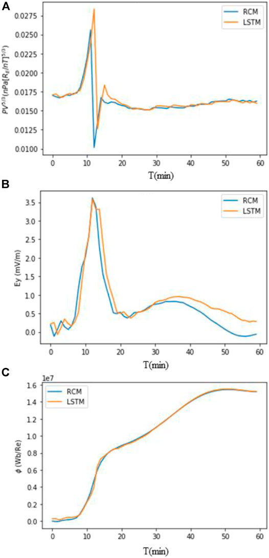
FIGURE 4. Single-point comparison of the RCM single bubble run with the LSTM-based RNN model at X = −9.9 and Y = −1.1; (A) PV5/3 in nPa [Re/nT]5/3; (B) Ey in mV/m; and (C)ϕ in Wb/Re.
In general, CMFT shows a better match between the LSTM and the RCM simulation; however, there are some tiny timescale deviations between the LSTM and the RCM for Ey and PV5/3. In all the solution times presented in this section, we see that the CMFT is the only parameter that steadily grows along the bubble propagation path with time. The LSTM-based algorithms have minimal errors while learning the time series trends of the parameters which start from a small or zero numerical value and tend to achieve a high numerical value with time (Eck and Schmidhuber, 2002).
Results
In this section, we will compare the LSTM forecast with the RCM single bubble simulation in the entire 2-D equatorial plane for all three simulations, focusing on the latter 30 min.
Figure 5 shows the single bubble injection run for T = 31 min. At this time, the bubble injection has already been completed in the plasma sheet, although variations in PV5/3 (Figure 5A) and Ey (Figure 5B) are still visible along the injection path. Figure 5C shows a significant enhancement in the CMFT in yellow-red color from X = −5 to X = −16 Re. The LSTM modeling reproduces the distribution of these three key parameters very well, even for the small-scale fluctuations. In order to check the forecast and the quality of prediction, we also compare the RCM and the LSTM model at different solution times to check if the LSTM forecast is updating and able to track the changes that are evolving in the RCM simulation with time. Figures 6, 7 compare the two modeling results, 11 and 21 min after the training solution time, respectively. The LSTM forecasts reasonably resemble the RCM simulation. It can be seen that the residual fluctuations in the electric field Ey and the associated structures in the CMFT ϕ can also be reproduced in the LSTM model.
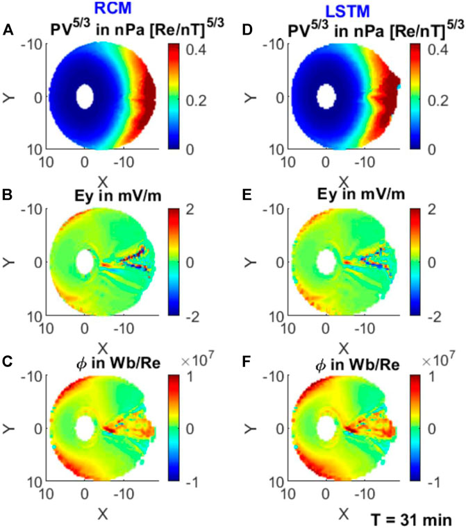
FIGURE 5. Comparison of the RCM single bubble injection run (left) with the LSTM forecast (right). From top to bottom are PV5/3, Ey, and ϕ at T = 31 min.
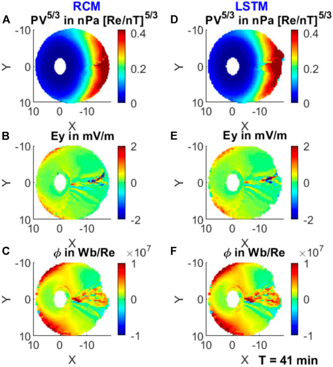
FIGURE 6. Similar to Figure 5, but for T = 41 min.
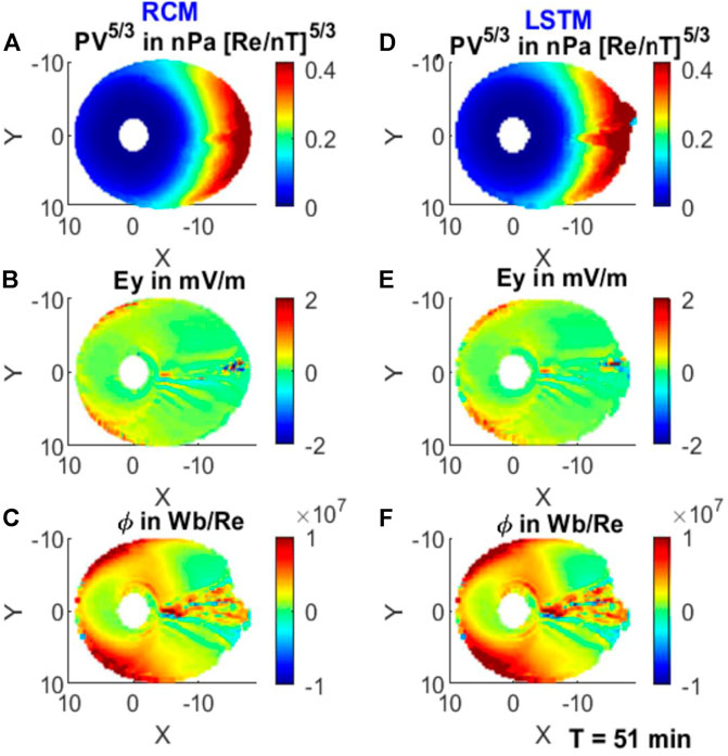
FIGURE 7. Similar to Figure 5, but for T = 51 min.
Furthermore, we would like to compare the LSTM forecast with the RCM results at the end of the simulation time. The LSTM model has used part of the RCM simulation as an input; therefore, the LSTM forecast performance must be checked beyond the 30 min training solution time and up to the end of the RCM simulation. Comparison of the end solution time of the single bubble RCM simulation to the LSTM forecast will boost the confidence of the LSTM-based RNN model for its further development and extensive use in parallel to the RCM simulation. Similar to previous times, the LSTM forecast is very consistent with the RCM results, as shown in Figure 8.
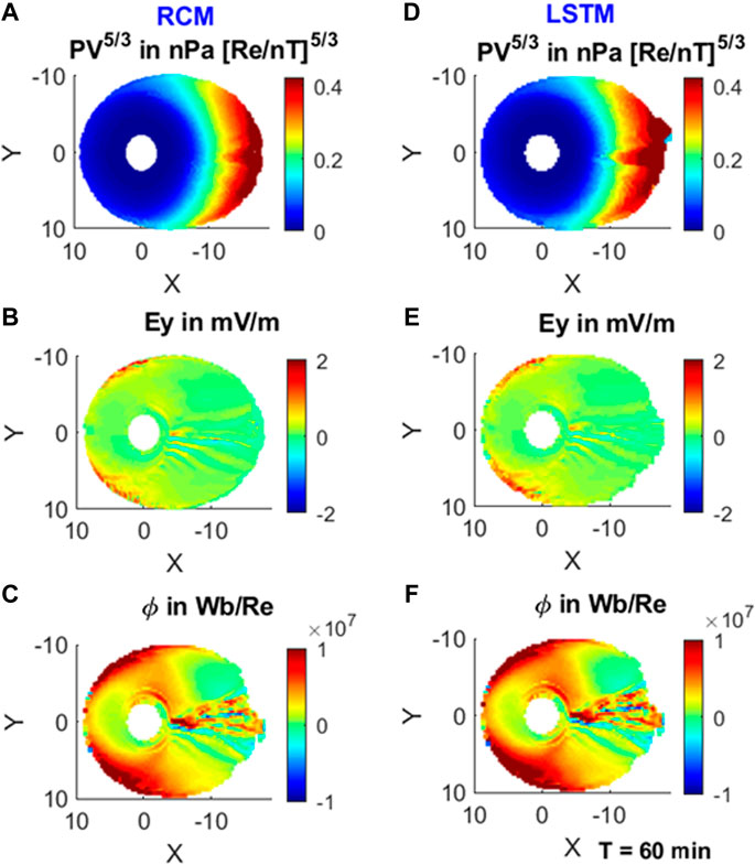
FIGURE 8. Similar to Figure 5, but for T = 60 min.
Similar to the above case, we have applied the same approach to predict the RCM simulation results for the single-flow-channel run and the three-flow-channel run. Again, we have trained the LSTM model for the first 30 min and forecasted the next 30 min. Figures 9A–D and Figures 9E–H are similar to Figure 2 and Figure 3. This figure compares the single flow channel and the three flow channels at T = 7 min. In Figures 8A–D, the changes in the modeled parameters appear at one point near the magnetic midnight in the equatorial plane. However, for the three flow channels (Figures 9E–H), the changes related to the launch of the three flow channels are present at the three points, and it is consistent in all four modeled parameters. This figure is also useful as it is reproducing the RCM simulation for the two different cases whose simulation time is within the boundary condition for both the runs.
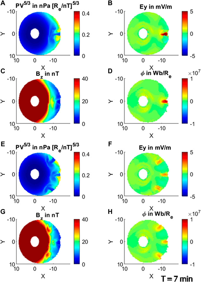
FIGURE 9. Similar to Figure 2 or Figure 3, from A–D is for the single flow channel and E–H is for the three flow channels at T = 7 min.
As discussed earlier, for the single bubble run, the LSTM and the forecast have to be compared at different times for the single-flow-channel and three-flow-channel runs. Figures 10, 11 compare the four RCM parameters as compared in Figures 5–8. But this time, we compared the PV5/3 at T = 32 min, Ey at T = 41 min, and CMFT at T = 49 min. The inputs provided within the simulation boundary conditions triggered LSTM fast learning of the correlation between different parameters and the degree and order of their mutual variance. We also train the LSTM model a little beyond the boundary condition of the LSTM, which allows the forget gate to classify the frequency of spatial and temporal vanishing gradients among the input parameters in the time series. LSTM forecasts were fully replicating the changes in the modeled parameters at and around the flow channel existence regions, at the boundary layer and near the geosynchronous orbit. In all the three simulation times and the runs presented in the study, there is a good agreement between the RCM simulation and the LSTM forecast for the three modeled parameters. These comparative pieces of evidence indicate that the LSTM is a strong data learning tool when it comes to learning large time series multivariate data trends, in particular when the variables in the data trends are related to each other by well-defined physics. LSTM’s supervised learning algorithm makes it capable of extracting the degree of underlying correlation among many variables of a multiparameter data series through clustering, dimensionality reduction, structured prediction, and reinforcement learning.
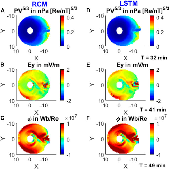
FIGURE 10. From top to bottom are comparison of the RCM and LSTM forecasts during the single-flow-channel run for PV5/3 at T = 32 min, Ey at T = 41 min, and ϕ at T = 49 min.
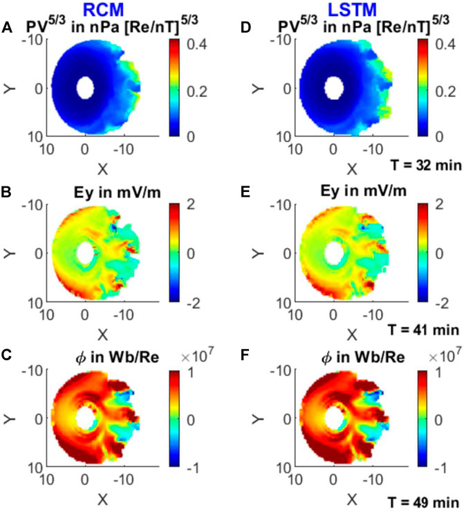
FIGURE 11. Similar to Figure 10, but for the three-flow-channel run.
LSTM Forecast Error Analysis
To check and quantify the error in the LSTM prediction of the RCM simulations during three different runs, we have calculated the correlation coefficient (Corr), which is used to study the statistical relationship between two parameters: the mean absolute error (MAE), which is an arithmetic average of the absolute error, and the mean squared error or mean squared deviation (MSE), which is the mean of the squares of the errors and is used for checking the quality of a procedure or method to predict an observed/simulated quantity (Chai and Draxler, 2014). The root mean square error (RMSE) is widely used to measure the difference between the predicted or estimated value, using a model or an estimator with respect to the observed or simulated value. The RMSE is the square root of the second sample moment of the difference between predicated and observed/simulated values or the quadratic mean of these differences (Chai and Draxler, 2014 and references therein). We calculated the Corr, MAE, MSE, and RMSE for the 30–60 min of the RCM simulation and the LSTM forecast all through the three simulations presented. We have divided the space/time into four sectors using the magnetic local time (MLT) range. The four sectors are magnetic dawn (03:00–09:00 MLT), magnetic noon (09:00–15:00 MLT), magnetic dusk (15:00–21:00 MLT), and magnetic midnight (21:00–03:00 MLT). Table 1 shows the calculated error for the single bubble run. Similarly, Tables 2, 3 show the Corr, MAE, MSE, and RMSE for the 30–60 min for the single-flow-channel run and the three-flow-channel run.
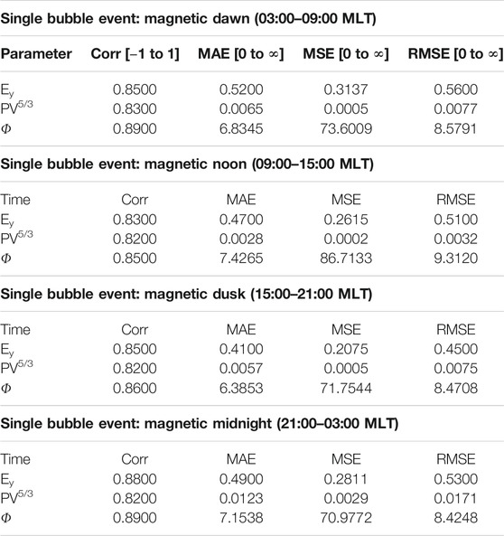
TABLE 1. Error Analysis for Single Bubble injection.
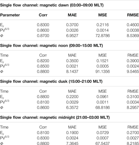
TABLE 2. Error Analysis for Single Flow Channel.
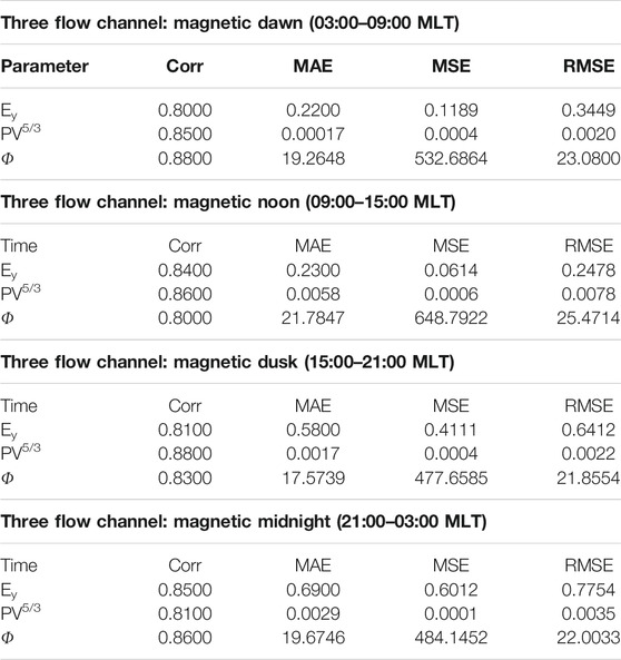
TABLE 3. Error Analysis for Three Flow Channel.
The Corr for all the runs and for all the parameters is more than 0.80, which indicates that the LSTM forecast is in a good statistical coherence to the RSM simulations. The Corr for the CMFT is comparatively high as it is overall positive, and it has an increasing trend from a very low value, which makes it easier for LSTM to learn and reproduce the variation trend as compared to the Ey and PV5/3. The correlation coefficient is close to 1, which also indicates the linear statistical relationship between the LSTM forecast and the RCM simulation.
RMSE and MAE are two variables used to measure the accuracy between the two continuous variables, and RMSE and MAE can vary between 0 and ∞. The MAE uses the absolute difference between the observation and prediction. The numerical value of the MAE and the RMSE is considered well for a prediction if it is close to zero. The MAE is highly dependent on the magnitude of the two continuous variables for which the MAE is calculated. The RMSE uses the quadratic scoring rule, and it also measures the error. Both the MAE and the RMSE measure the average model prediction error regardless of considering the direction of prediction. The RMSE and MAE are always in the unit of the predicted/observed variable. If we compare the MAE and RMSE values for Ey, PV5/3, and ϕ, they seem to be in coherence with these three plasma sheet parameters.
RMSE values are generally higher than those of the MAE because the RMSE uses the squared errors before averaging; therefore, it gives more weight to the higher value errors. It is hard to see any trend in the RMSE and MAE for the three different runs at the four MLT sectors that are discussed in the study; however, it is noticeable that with the increased number of flow channels, the RMSE, MSE, and MAE have increased significantly. This enhancement indicates that with an increasing number of flow channels, it becomes challenging for the LSTM model to forecast the RCM simulation. It is because each flow channel or each bubble influences the entire modeled region and when there is a greater number of flow channels and bubbles, LSTM-based models need to assess the influence due to all the flow channels, considering their launch location and the duration they exist for. We have also used the MSE, which is generally used to evaluate the quality of the predictor or estimator. The MSE is in the squared unit of the observed parameter, as it is the second moment of the errors. The MSE shows the variance of the estimator or model and shows the error as the square of the quantity being measured. In all the cases and MLT sectors, the MSE is close to the square of the RMSE, which is consistent with all the other error analyses in the presented study.
Concluding Remarks and Summary
The presented LSTM method is applied to build a parallel statistical model using a physics-based magnetospheric model like the RCM. There are other kinds of models which rely on the observation data from the satellite and/or coupled with the ground-based observation. The LSTM-based models can be applicable to both physics-based models and analytical models dependent on the observational data.
The three case studies (i.e., single bubble, one flow channel, and three flow channels) presented in this article reflect that just after LSTM was trained with the initial simulation results from the RCM LSTM model, it was able to accurately replicate the 60 min RCM simulations. All the three LSTM models were able to forecast temporal and spatial variations in entropy parameter PV5/3, dawn-to-dusk electric field Ey, and CMFT ϕ. The LSTM forecast quality was very satisfactory from the beginning until the end of the forecast. The performance of the LSTM model for the near-Earth plasma sheet parameter forecast in this study demonstrates that the LSTM is a powerful RNN tool that can be applied to any time series scientific data to learn the underlying relationship among many scientific parameters and to forecast any desired scientific parameters until the produced forecasts fully abide by the scientific laws.
The main limitation of the LSTM models is their dependence on the input data that come from real observation or a physics-based model’s simulation. Besides this, if the LSTM model is multivariate (as in our case), one must find the best sequence of the input parameters in terms of the degree of their dependence on the parameter to be predicted. On the other hand, once these two discussed steps are accomplished, the LSTM multivariate algorithm is powerful in learning the underlying trends among the input variables. However, these LSTM models must still be trained up to the boundary condition implementation in the RCM simulation, in order to produce reasonable and reliable forecasts. Beyond the RCM simulation’s boundary condition, the LSTM models are great in producing similar variation trends to the RCM simulations.
In both cases, LSTM will need a significant amount of the model inputs. The first step before training the LSTM algorithm is to logically choose the best inputs and their order, which influence model outputs the most. It can be done in two ways. First, if the physical parameters we are going to model can be written in the form of mathematical equations, then we know on what it depends the most, and we prepare the input order accordingly. But, in case there are two or more input parameters, we can use different combinations of their orders and compare the root mean square error (RMSE) of all the outputs. The input combination with the least RMSE is the best model. For training the LSTM algorithm in parallel to an existing model, it is challenging and crucial to choose the appropriate training and test duration. The modeler should make sure that all the boundary conditions must fall within the training duration for the model, and they should also train the model by allowing it to learn the underlying relationship between the different inputs once all the boundary conditions are defined. In the presented case studies, all the boundary conditions are defined within the first quarter of simulation time, and the LSTM model is trained for the initial 30 min. Now, at this point, we can test the model by splitting the entire dataset into the train and test periods, which means we train the LSTM model with part of the data and then forecast the remaining time series, which is compared to the input data beyond the training time limit. If there is a good match in the forecast and observation, we can fit this model for the entire dataset, and the last LSTM product would be the final model, which can forecast the entire data series.
Here, the readers should keep in mind that the presented LSTM approach is to study an RCM simulation and not the general trend of variation of the inner magnetosphere and/or plasma sheet parameters. Therefore, for a distinct kind of RCM simulation (or other physics-based models), we must develop the distinct input datasets and fit the LSTM model over it. For the analytical model, it can prove itself to be more superior by learning the long-term data trend during the different kinds of solar activity, and it can be developed to forecast a few years of the data in a few easy steps. For example, there is a time delay in the ionospheric response for dayside and nightside as when the interplanetary magnetic field (IMF) turns from northward to southward, the IMF is measured at the dayside (Tenfjord et al., 2017). Therefore, if we have real-time solar wind data, LSTM can be used to develop an alarm for the hazardous events before an hour or so. The physics-based model and the analytical model dependent on observations are costlier in terms of their computational costs and the huge amount of time and resources spent in developing and maintaining them. On the other hand, the LSTM-based modeling algorithm is purely statistical and nonscientific in general. But the LSTM can be made scientific by training it to learn the underlying relationship of any existing models’ inputs. Once we are sure that the LSTM outputs satisfy the scientific conditions and the produced outputs are satisfactory to our goals, it can be used as a parallel forecasting/nowcasting system to any space weather or magnetospheric model.
Three RCM simulation (single bubble, single flow channel, and three flow channels) runs’ 50% data are used to train a multivariate LSTM model for the three plasma sheet parameters. The LSTM forecast is tested within the boundary condition and beyond the boundary condition of the 60 min simulation. For all the simulation times, there was a good agreement between the RCM simulation and LSTM forecast. All the major and minor fluctuations in the RCM parameters were fully noticeable at all the times and regions of the RCM simulation. The inner magnetospheric data are limited, and it is hard to build a statistical model using the available satellite data (e.g., THEMIS, MMS, ERG, and Cluster II). On the other hand, the RCM is a well-established physics-based model, and we can produce any type of the run according to our need and concern. The RCM-simulated results are stable for the deep learning–based statistical modeling, and the input environment is well known. These merits of the RCM simulation boundary conditions make them suitable inputs for the LSTM-based RNN model of the inner magnetospheric parameters. Here in this study, it is the very first time a magnetospheric modeled output is being used in the recurrent neural network for forecasting. We have used RCM single bubble, single flow channel, and multiple flow channel runs for the initial 30-min simulation to train our LSTM model. We developed three independent deep learning models for entropy parameter, dawn-to-dusk electric field, and cumulative magnetic flux transport. We have validated the LSTM model by comparing its single point’s prediction time series with the RCM single bubble, one-flow-channel, and three-flow-channel runs, the single-point time series simulations. We found a great coherence in both the models (RCM and LSTM). Later, we used 2D maps in the X and Y coordinates to compare the LSTM forecast to the RCM simulation at distinct solution times. In all the solution times, the LSTM forecasts demonstrate a good agreement with the RCM output for all three inner magnetospheric parameters modeled.
The CMFT comes out as the only parameter that steadily grows along the bubble propagation path with time. The LSTM-based algorithms are more appropriate for modeling such parameters which start from a small numerical value and have a tendency to achieve a high numerical value with time. Overall, the LSTM predicted that all parameters are in good prediction range as compared to the RCM simulations. The most significant part of the presented modeling approach was that the prediction efficiency did not compromise with time. The LSTM forecast’s efficiency was very satisfactory within and beyond the boundary condition run time. The forecasted parameters through the LSTM were spatially evolving in the same way as in the RCM simulation, and we are confident that the LSTM can be used to train and predict different sophisticated runs of the inner magnetospheric parameters in the future.
Data Availability Statement
The raw data supporting the conclusions of this article will be made available by the authors, without undue reservation.
Author Contributions
SP planned the research, developed the LSTM and RCM code, and wrote the manuscript. JY helped in editing the manuscript, revising it, and reshaped several of its sections. WS helped in the plasma bubble simulation launch and provided technical details related to it.
Funding
This work at the Southern University of Science and Technology was supported by grant no. 41974187 of the National Natural Science Foundation of China (NSFC) and grant no. XDB41000000 of the Strategic Priority Research Program of the Chinese Academy of Science.
Conflict of Interest
The authors declare that the research was conducted in the absence of any commercial or financial relationships that could be construed as a potential conflict of interest.
References
Angelopoulos, V., Baumjohann, W., Kennel, C. F., Coroniti, F. V., Kivelson, M. G., Pellat, R., et al. (1992). Bursty Bulk Flows in the Inner central Plasma Sheet. J. Geophys. Res. 97 (A4), 4027–4039. doi:10.1029/91JA02701
Baker, D. N., McPherron, R. L., Cayton, T. E., and Klebesadel, R. W. (1990). Linear Prediction Filter Analysis of Relativistic Electron Properties at 6.6 RE. J. Geophys. Res. 95 (15), 133. doi:10.1029/ja095ia09p15133
Birn, J., Liu, J., Runov, A., Kepko, L., and Angelopoulos, V. (2019). On the Contribution of Dipolarizing Flux Bundles to the Substorm Current Wedge and to Flux and Energy Transport. J. Geophys. Res. Space Phys. 124, 5408–5420. doi:10.1029/2019JA026658
Camporeale, E. (2019). The Challenge of Machine Learning in Space Weather: Nowcasting and Forecasting. Space Weather 17, 1166–1207. doi:10.1029/2018SW002061
Chai, T., and Draxler, R. R. (2014). Root Mean Square Error (RMSE) or Mean Absolute Error (MAE)? - Arguments against Avoiding RMSE in the Literature. Geosci. Model. Dev. 7, 1247–1250. doi:10.5194/gmd-7-1247-2014
Connor, J. T., Martin, R. D., and Atlas, L. E. (1994). Recurrent Neural Networks and Robust Time Series Prediction. IEEE Trans. Neural Netw. 5 (2), 240–254. doi:10.1109/72.279188
Eck, D., and Schmidhuber, J. (2002). A First Look at Music Composition Using LSTM Recurrent Neural Networks. Istituto Dalle Molle Di Studi Sull Intelligenza Artificiale 103, 1–11.
Gers, F. A., Schmidhuber, J., and Cummins, F. (2000). Learning to Forget: Continual Prediction with LSTM. Neural Comput. 12 (10), 2451–2471. doi:10.1162/089976600300015015
Graves, A., Mohamed, A.‐R., and Hinton, G. (2013). “Speech Recognition with Deep Recurrent Neural Networks,” in 2013 IEEE International Conference on Acoustics, Speech and Signal Processing, Vancouver, BC, Canada, May 26–31, 2013(IEEE), 6645–6649.
Graves, A., and Schmidhuber, J. (2005). Framewise Phoneme Classification with Bidirectional LSTM and Other Neural Network Architectures. Neural Networks 18 (5‐6), 602–610. doi:10.1016/j.neunet.2005.06.042
Khotyaintsev, Y. V., Cully, C. M., Vaivads, A., André, M., and Owen, C. J. (2011). Plasma Jet Braking: Energy Dissipation and Nonadiabatic Electrons. Phys. Rev. Lett. 106 (16), 165001. doi:10.1103/PhysRevLett.106.165001
Kitamura, K., Nakamura, Y., Tokumitsu, M., Ishida, Y., and Watari, S. (2011). Prediction of the Electron Flux Environment in Geosynchronous Orbit Using a Neural Network Technique. Artif. Life Robotics 16 (3), 389–392. doi:10.1007/s10015‐011‐0957‐1
Koon, H. C., and Gorney, D. J. (1991). A Neural Network Model of the Relativistic Electron Flux at Geosynchronous Orbit. J. Geophys. Res. 96, 5549–5559. doi:10.1029/90JA02380
Lemon, C., Wolf, R. A., Hill, T. W., Sazykin, S., Spiro, R. W., Toffoletto, F. R., et al. (2004). Magnetic Storm Ring Current Injection Modeled with the Rice Convection Model and a Self-Consistent Magnetic Field. Geophys. Res. Lett. 31, L21801, 1–4. doi:10.1029/2004GL020914
Ling, A. G., Ginet, G. P., Hilmer, R. V., and Perry, K. L. (2010). A Neural Network-Based Geosynchronous Relativistic Electron Flux Forecasting Model. Space Weather 8, S09003, 1–14. doi:10.1029/2010SW000576
Liu, J., Angelopoulos, V., Runov, A., and Zhou, X.-Z. (2013). On the Current Sheets Surrounding Dipolarizing Flux Bundles in the Magnetotail: The Case for Wedgelets. J. Geophys. Res. Space Phys. 118, 2000–2020. doi:10.1002/jgra.50092n
McIlwain, C. E. (1972). “Plasma Convection in the Vicinity of the Geosynchronous Orbit,” in Earth’s Magnetospheric Processes. Editor B. M. McCormac (Dordrecht, Netherlands: D. Reidel), 268–279.
McIlwain, C. E. (1974). “Substorm Injection Boundaries,” in Magnetospheric Physics. Editor B. M. McCormac (Dordrecht, Netherlands: D. Reidel), 143–154.
Nakamura, R., Baumjohann, W., Klecker, B., Bogdanova, Y., Balogh, A., Rème, H., et al. (2002). Motion of the Dipolarization Front during a Flow Burst Event Observed by Cluster. Geophys. Res. Lett. 29 (20), 3–1. doi:10.1029/2002GL015763
Pedregosa, F., Varoquaux, G., Gramfort, A., Michel, V., Thirion, B., Grisel, O., et al. (2011). Scikit-learn: Machine Learning in python. J. Mach. Learn. Res. 12, 2825–2830.
Pires de Lima, R., Chen, Y., and Lin, Y. (2020). Forecasting Megaelectron‐Volt Electrons inside Earth's Outer Radiation Belt: PreMevE 2.0 Based on Supervised Machine Learning Algorithms. Space Weather 18, e2019SW002399. doi:10.1029/2019SW002399
Pontius, D. H., and Wolf, R. A. (1990). Transient Flux Tubes in the Terrestrial Magnetosphere. Geophys. Res. Lett. 17 (1), 49–52. doi:10.1029/GL017i001p00049
Runov, A., Angelopoulos, V., Sitnov, M. I., Sergeev, V. A., Bonnell, J., McFadden, J. P., et al. (2009). THEMIS Observations of an Earthward-Propagating Dipolarization Front. Geophys. Res. Lett. 36, L14106. doi:10.1029/2009GL038980
Shin, D.-K., Lee, D.-Y., Kim, K.-C., Hwang, J., and Kim, J. (2016). Artificial Neural Network Prediction Model for Geosynchronous Electron Fluxes: Dependence on Satellite Position and Particle Energy. Space Weather 14 (4), 313–321. doi:10.1002/2015SW001359
Silin, I., Toffoletto, F., Wolf, R., and Sazykin, S. Y. (2013). “Calculation of Magnetospheric Equilibria and Evolution of Plasma Bubbles with a New Finite‐volume MHD/magnetofriction Code,” in American Geophysical Union, Fall Meeting 2013, San Francisco, December 9–13, 2013, SM51B‐2176.
Stringer, G. A., Heuten, I., Salazar, C., and Stokes, B. (1996). Artificial Neural Network (ANN) Forecasting of Energetic Electrons at Geosynchronous Orbit. Washington, DC, USA: American Geophysical Union, 291–295. doi:10.1029/GM097p0291
Tenfjord, P., Østgaard, N., Strangeway, R., Haaland, S., Snekvik, K., Laundal, K. M., et al. (2017). Magnetospheric Response and Reconfiguration Times Following IMF B Y Reversals. J. Geophys. Res. Space Phys. 122, 417–431. doi:10.1002/2016JA023018
Toffoletto, F., Sazykin, S., Spiro, R., and Wolf, R. (2003). Inner Magnetospheric Modeling with the Rice Convection Model. Space Sci. Rev. 107, 175–196. doi:10.1007/978-94-007-1069-6_19
Ukhorskiy, A. Y., Sitnov, M. I., Sharma, A. S., Anderson, B. J., Ohtani, S., and Lui, A. T. Y. (2004). Data-derived Forecasting Model for Relativistic Electron Intensity at Geosynchronous Orbit. Geophys. Res. Lett. 31 (9), L09806, 1–4. doi:10.1029/2004GL019616
Wei, L., Zhong, Q., Lin, R., Wang, J., Liu, S., and Cao, Y. (2018). Quantitative Prediction of High-Energy Electron Integral Flux at Geostationary Orbit Based on Deep Learning. Space Weather 16 (7), 903–916. doi:10.1029/2018SW001829
Weimer, D. R. (2005). Improved Ionospheric Electrodynamic Models and Application to Calculating Joule Heating Rates. J. Geophys. Res. 110, A05306. doi:10.1029/2004ja010884
Wiltberger, M., Rigler, E. J., Merkin, V., and Lyon, J. G. (2017). Structure of High Latitude Currents in Magnetosphere-Ionosphere Models. Space Sci. Rev. 206, 575–598. doi:10.1007/s11214-016-0271-2
Yang, J., Toffoletto, F. R., Erickson, G. M., and Wolf, R. A. (2010a). Superposed Epoch Study ofPV5/3during Substorms, Pseudobreakups and Convection Bays. Geophys. Res. Lett. 37, L07102, 1–5. doi:10.1029/2010GL042811
Yang, J., Toffoletto, F. R., and Song, Y. (2010b). Role of Depleted Flux Tubes in Steady Magnetospheric Convection: Results of RCM-E Simulations. J. Geophys. Res. 115, A00I11, 1–10. doi:10.1029/2010JA015731
Yang, J., Toffoletto, F. R., and Wolf, R. A. (2016). Comparison Study of Ring Current Simulations with and without Bubble Injections. J. Geophys. Res. Space Phys. 121, 374–379. doi:10.1002/2015JA021901
Yang, J., Toffoletto, F. R., Wolf, R. A., and Sazykin, S. (2011). RCM-E Simulation of Ion Acceleration during an Idealized Plasma Sheet Bubble Injection. J. Geophys. Res. 116, A05207. doi:10.1029/2010JA016346
Yang, J., Toffoletto, F. R., Wolf, R. A., and Sazykin, S. (2015). On the Contribution of Plasma Sheet Bubbles to the Storm Time Ring Current. J. Geophys. Res. Space Phys. 120, 7416–7432. doi:10.1002/2015JA021398
Keywords: machine learning, substorm injections, numerical simulation, plasma sheet, M-I coupling
Citation: Priyadarshi S, Yang J and Sun W (2021) Modeling and Prediction of Near-Earth Plasma Sheet Parameters Using the Rice Convection Model and the Recurrent Neural Network. Front. Astron. Space Sci. 8:691000. doi: 10.3389/fspas.2021.691000
Received: 05 April 2021; Accepted: 17 May 2021;
Published: 09 June 2021.
Edited by:
Jean-Francois Ripoll, CEA DAM Île-de-France, FranceReviewed by:
Alexei V. Dmitriev, Lomonosov Moscow State University, RussiaBinbin Tang, National Space Science Center (CAS), China
Copyright © 2021 Priyadarshi, Yang and Sun. This is an open-access article distributed under the terms of the Creative Commons Attribution License (CC BY). The use, distribution or reproduction in other forums is permitted, provided the original author(s) and the copyright owner(s) are credited and that the original publication in this journal is cited, in accordance with accepted academic practice. No use, distribution or reproduction is permitted which does not comply with these terms.
*Correspondence: Jian Yang, eWFuZ2ozNkBzdXN0ZWNoLmVkdS5jbg==; Shishir Priyadarshi, cHJpeWFkYXJzaGlAc3VzdGVjaC5lZHUuY24=