A Novel Magnetosphere–Ionosphere Coupling Model for the Onset of Substrom Expansion Phase

A novel magnetosphere–ionosphere (M-I) coupling model is proposed to simulate the brightening of the onset auroral arc of a magnetospheric substorm event. The new M-I coupling model is modified from the M-I coupling model proposed by the Alaska research team in 1988. We adjust the magnetospheric boundary conditions by including the Hall effects in the thin current sheet and allowing the spatial distributions of the reflection–transmission coefficient to vary with time. As a result, brightening and poleward drifting of multiple auroral arcs appear for the first time in an M-I coupling model. The new results indicate that the coupled Hall effects in the near-Earth plasma sheet and the E-region ionosphere play a vital role in triggering the onset of a magnetospheric substorm.

Introduction

Kan and Sun. (1985), Kan et al. (1988), and Kan and Sun. (1996) have proposed a highly simplified but an elegant simulation scheme to model the substorm-associated magnetosphere–ionosphere (M-I) coupling processes. Their results show a plasma flow pattern similar to the observed westward traveling surge during the substorm. The cross-polar-cap potential drop in the E-region ionosphere obtained in their model is slightly lower than the initial input cross-polar-cap potential drop. The nonuniform distributions of the conductivities and electric fields in the E-region ionosphere can result in the region-1 and region-2 field-aligned current distributions (e.g., Iijima and Potemra, 1976). Similar results have been obtained in the M-I coupling simulations studied by Miura and Sato. (1980); Miura and Sato. (1981). However, these early simulation studies (e.g., Miura and Sato, 1980, Miura and Sato, 1981); (Kan and Sun, 1985; Kan et al., 1988) fail to show onset aurora arc–associated upward field-aligned currents in the midnight region (e.g., Akasofu, 1964).

Kan and Sun. (1996) changed the conductivity enhancement scheme and modified the convection electric field by adding localized convection electric fields on the magnetotail boundary of the M-I coupling model. They successfully obtain upward field-aligned currents in the midnight region (Kan and Sun, 1996).

Based on satellite observations, the near-Earth plasma sheet shows a tail-like structure before the onset of a substorm. It changes to a dipole-like structure after the onset of the substorm (e.g., McPherron, 1972). Kaufmann. (1987) showed that the dipolarization of the near-Earth plasma sheet at the onset of a substorm is associated with the formation of current wedges. Dipolarization of the magnetic field occurs inside the current wedges, whereas the thinning processes continuously take place outside of the current wedges and tailward from the current wedges (Kaufmann, 1987). Ohtani et al. (1992) found several substorm onset events with explosive thinning of the plasma sheet before the onset of substorms.

It is believed that disruption of cross-tail currents in the near-Earth plasma sheet can trigger the dipolarization process. Theoretical models have been proposed to explain the current disruption in the near-Earth plasma sheet. These theoretical models include, but not limited to, the magnetic reconnection–associated resistive tearing-mode instability (e.g., Furth et al., 1963; Coppi et al., 1966; Schindler, 1974), the ion Weibel instability (e.g., Lui et al., 1993; Lui et al., 2008), the ballooning instability (e.g., Roux et al., 1991; Cheng and Lui, 1998), and the unloading instability triggered by the incident Alfvén waves from the ionosphere (Kan and Sun, 1996). Lyu and Chen. (2000) proposed another type of unloading instability due to the M-I coupling process and the nonuniform Hall effect in the explosively thinning region.

When a current sheet has a finite normal magnetic field component, and when the thickness of the current sheet is equal to or smaller than the gyroradius of the thermal ions, a sufficient amount of ions will become unmagnetized, whereas electrons are still magnetized. The unmagnetized ions will move across the thin current sheet along the electric field direction with a meandering trajectory. Magnetized electrons and unmagnetized ions will set up a Hall electric field along the drift direction of the magnetized electrons. As a result, the electric field will rotate left-handed with respect to the ambient magnetic field. If the thickness of the current sheet is nonuniform, it can lead to a nonuniform left-handed rotation of the electric field and results in localized field-aligned currents. The upward field-aligned current from the ionosphere to the thin current sheet in the pre-midnight region can increase the normal magnetic field component in the thin current sheet downward from the field-aligned current. Since the meandering motion of ions in the thin current sheet can enhance the cross-tail current intensity, increasing the current sheet thickness will reduce the number of unmagnetized ions. Decreasing the number of unmagnetized ions can reduce the cross-tail current intensity and further increase the current sheet thickness. This positive feedback process can result in current disruption and trigger the onset of a substorm (Lyu and Chen, 2000).

Unlike the other instabilities analyses, where waves of a given frequency are amplified with a well-determined growth rate, the unloading instability proposed by Lyu and Chen. (2000) does not have a well-defined growth rate or a well-defined frequency. Since the background magnetic field of the unloading instability is highly nonuniform and time dependent, we can only qualitatively show a positive feedback process to trigger the current disruption in the thin current sheet.

This study aimed to modify the M-I coupling model proposed by Kan et al. (1988) by including the Hall effects in the magnetotail as proposed by Lyu and Chen. (2000). The coupling between the nonuniform Hall effect in the high-latitude E-region ionosphere and the nonuniform Hall effect on the magnetospheric boundary will be examined.

Basic Equations of the Magnetosphere–Ionosphere Coupling Model

The new M-I coupling model is modified from the M-I coupling model proposed by Kan et al. (1988). For convenience, we shall call the M-I coupling model proposed by Kan et al. (1988) as the KZA′88 model. The high-latitude ionosphere in the KZA′88 model is a plane with uniform magnetic field B₀ perpendicular to the ionosphere. The nonuniform electric fields and conductivities yield nonuniform electrical currents in the high-latitude ionosphere. Since no charge accumulation could take place in the timescale of the KZA′88 model, the divergence of the height-integrated perpendicular current density in the E-region ionosphere implies a downward field-aligned current at the top of the E-region ionosphere. Likewise, the convergence of the height-integrated perpendicular current density can lead to an upward field-aligned current at the top of the E-region ionosphere. The upward field-aligned current $J_z$ at the top of the E-region ionosphere can be written in the following form (e.g., Kan et al., 1988).

$J_z=-{\nabla }_{\perp }\cdot \left({\displaystyle {\Sigma }_P{\mathit{E}}_i+{\Sigma }_H{\widehat{B}}_0\times {\mathit{E}}_i}\right),(1)$

where ${\widehat{B}}_0$ is the unit vector parallel to ${\mathit{B}}_0$, ${\Sigma }_P$ is the height-integrated Pedersen conductivity, ${\Sigma }_H$ is the height-integrated Hall conductivity, and ${\mathit{E}}_i$ is the vertical averaged electric field in the E-region ionosphere. The direction of ${\mathit{E}}_i$ is perpendicular to the background magnetic field ${\mathit{B}}_0$ in this study.

The coupling between the ionosphere and the magnetosphere in the KZA′88 model is achieved by the Alfvén waves that carry the electric field and field-aligned current and propagate back and forth between these two regions along the magnetic field lines. Based on the Walén relation (Walén, 1944), Kan and Sun. (1985) have shown that the Alfvén waves with group velocity parallel to the background magetic field will carry field-aligned currents:

$J_{\parallel 1}=+{\displaystyle {\Sigma }_A\nabla \cdot {\mathit{E}}_{\perp 1}},(2)$

where $J_{\parallel 1}={\widehat{B}}_0\cdot \nabla \times {\mathit{B}}_1/{\mu }_0$, ${\mathit{B}}_1$ is the perturbed magnetic field in the Alfvén wave, ${\Sigma }_A=1/{\mu }_0{V}_{A0}$ is the effective height-integrated conductivity in the Alfvén wave, $V_{A0}=B_0/\sqrt{{\mu }_0{\rho }_0}$ is the Alfvén speed, ${\rho }_0$ is the background plasma mass density, and ${\mathit{E}}_{\perp 1}$ is the perpendicular component of the perturbed electric field in the Alfvén wave. Likewise, Alfvén waves with group velocity antiparallel to the background magnetic field will carry field-aligned currents:

$J_{\parallel 1}=-{\displaystyle {\Sigma }_A\nabla \cdot {\mathit{E}}_{\perp 1}}.(3)$

Since the background magnetic field is downward in the northern hemisphere high-latitude ionosphere, we have $J_{\parallel 1}=-J_{z1}$, and the group velocity of the incident Alfvén wave is parallel to the background magnetic field, whereas the group velocity of the reflected Alfvén wave is antiparallel to the background magnetic field. Thus, Eqs 2, 3 yield

$-J_{z1}^I=+{\displaystyle {\Sigma }_A\nabla \cdot {\mathit{E}}_{\perp 1}^I},(4)$

$-J_{z1}^R=-{\displaystyle {\Sigma }_A\nabla \cdot {\mathit{E}}_{\perp 1}^R},(5)$

where ${\mathit{E}}_{\perp 1}^I$ is the perpendicular component of the perturbed electric field in the incident Alfvén wave, $J_{z1}^I$ is the upward field-aligned current carried by the incident Alfvén wave, ${\mathit{E}}_{\perp 1}^R$ is the perpendicular component of the perturbed electric field in the reflected Alfvén wave, and $J_{z1}^R$ is the upward field-aligned current carried by the reflected Alfvén wave.

The reflected Alfvén waves from the ionosphere are determined in the following way in the KZA′88 model. When the sum of the $J_{z1}^I$ carried by the incident Alfvén waves and the preexisting field-aligned currents above the E-region ionosphere $J_{z0}$ do not match the required $J_z$ at the top of the E-region ionosphere, as shown in Eq. 1, Alfvén waves will be reflected from the ionosphere so that the upward field-aligned currents carried by the reflected Alfvén waves satisfy

$J_{z1}^R=J_z-\left(J_{z1}^I+J_{z0}\right).(6)$

According to Eq. 1, the preexisting field-aligned current $J_{z0}$ satisfies

$J_{z0}=-{\nabla }_{\perp }\cdot \left({\displaystyle {\Sigma }_{P0}{\mathit{E}}_{i0}}+{\displaystyle {\Sigma }_{H0}{\widehat{B}}_0\times {\mathit{E}}_{i0}}\right),(7)$

where ${\mathit{E}}_{i0}$, ${\Sigma }_{P0}$, and ${\Sigma }_{H0}$ are the preexisting ${\mathit{E}}_i$, ${\Sigma }_P$, and ${\Sigma }_H$, respectively.

Substituting Eqs 1, 4, 5, 7 into Eq. 6 to eliminate $J_z$, $J_{z1}^I$, $J_{z1}^R$, and $J_{z0}$, respectively, for the northern hemisphere ionosphere, it yields (Kan et al., 1988) the following equation:

${\displaystyle {\Sigma }_A\nabla \cdot {\mathit{E}}_{\perp 1}^R}=-{\nabla }_{\perp }\cdot \left({\displaystyle {\Sigma }_P{\mathit{E}}_i}+{\displaystyle {\Sigma }_H{\widehat{B}}_0\times {\mathit{E}}_i}\right)+{\displaystyle {\Sigma }_A\nabla \cdot {\mathit{E}}_{\perp 1}^I+{\nabla }_{\perp }}\cdot \left({\displaystyle {\Sigma }_{P0}{\mathit{E}}_{i0}}+{\displaystyle {\Sigma }_{H0}{\widehat{B}}_0\times {\mathit{E}}_{i0}}\right).(8)$

The electric field in the E-region ionosphere is determined in the following way in the KZA′88 model.

${\mathit{E}}_i=\left({\mathit{E}}_{i0}+{\mathit{E}}_{\perp 1}^I+{\mathit{E}}_{\perp 1}^R\right).(9)$

Substituting Eq. 9 into Eq. 8 to eliminate ${\mathit{E}}_i$ for the northern-hemisphere ionosphere, it yields

${\nabla }_{\perp }\cdot \left\{\left[\left({\Sigma }_P-{\Sigma }_{P0}\right)+\left({\Sigma }_H-{\Sigma }_{H0}\right){\widehat{B}}_0\times \right]{\mathit{E}}_{i0}+\left[\left({\Sigma }_P-{\Sigma }_A\right)+{\displaystyle {\Sigma }_H{\widehat{B}}_0}\times \right]{\mathit{E}}_{\perp 1}^I+\left[\left({\Sigma }_P+{\Sigma }_A\right)+{\displaystyle {\Sigma }_H{\widehat{B}}_0}\times \right]{\mathit{E}}_{\perp 1}^R\right\}=0.(10)$

Note that the KZA′88 model is modified from the M-I coupling model proposed by Kan and Sun. (1985). For convenience, we shall call the M-I coupling model proposed by Kan and Sun. (1985) as the KS′85 model. The matching conditions of the field-aligned currents and the perpendicular electric field used in the KS′85 model are given as follows:

$J_{z1}^R=\left(J_z-J_{z1}^I\right),(11)$

${\mathit{E}}_i=\left({\mathit{E}}_{\perp 1}^I+{\mathit{E}}_{\perp 1}^R\right).(12)$

Namely, both the preexisting field-aligned current $J_{z0}$ and the preexisting ionospheric perpendicular electric field ${\mathit{E}}_{i0}$ are ignored in the KS′85 model.

Since a current loop cannot last forever, especially when there is a finite Pederson conductivity in the E-region ionosphere, the current intensity in the preexisting current loop should decrease with time. In this study, we ignore the preexisting field-aligned current $J_{z0}$ and adopt the matching condition of the field-aligned currents used in the KS′85 model. On the other hand, the preexisting electric field ${\mathit{E}}_{i0}$ should be included in the M-I coupling model. When the preexisting electric field in the ionosphere is strong enough, the neutral particles might be pushed by the ions. Since the ionospheric conductivities are obtained in the neutral wind moving frame, we should determine the neutral wind flow velocity and modify the preexisting electric field to the neutral wind moving frame. However, modeling the enhanced neutral wind is beyond the scope of this study. We shall ignore the neutral wind effect and determine the electric field in the E-region ionosphere based on Eq. 9. Note that Kan and Sun (1996) also used Eqs 11, 9 instead of Eqs 6, 12 to match the field-aligned currents and to model the ionospheric electric field, respectively.

Substituting Eqs 1, 4, 5 into Eq. 11 to eliminate $J_z$, $J_{z1}^I$, and $J_{z1}^R$, respectively, for the northern-hemisphere high-latitude ionosphere, it yields the following equation:

${\displaystyle {\Sigma }_A\nabla \cdot {\mathit{E}}_{\perp 1}^R}=-{\nabla }_{\perp }\cdot \left({\displaystyle {\Sigma }_P{\mathit{E}}_i}+{\displaystyle {\Sigma }_H{\widehat{B}}_0\times {\mathit{E}}_i}\right)+{\displaystyle {\Sigma }_A\nabla \cdot {\mathit{E}}_{\perp 1}^I}.(13)$

Substituting Eq. 9 into Eq. 13 to eliminate ${\mathit{E}}_i$ for the northern-hemisphere ionosphere, it yields the following equation:

${\nabla }_{\perp }\cdot \left\{\left[{\text{Σ}}_P+{\text{Σ}}_H{\widehat{B}}_0\times \right]{\mathit{E}}_{i0}+\left[\left({\text{Σ}}_P-{\text{Σ}}_A\right)+{\text{Σ}}_H{\widehat{B}}_0\times \right]{\mathit{E}}_{\perp 1}^I+\left[\left({\text{Σ}}_P+{\text{Σ}}_A\right)+{\text{Σ}}_H{\widehat{B}}_0\times \right]{\mathit{E}}_{\perp 1}^R\right\}=0.(14)$

Eq. 14 yields

$\left[{\Sigma }_P+{\displaystyle {\Sigma }_H{\widehat{B}}_0}\times \right]{\mathit{E}}_{i0}+\left[\left({\Sigma }_P-{\Sigma }_A\right)+{\displaystyle {\Sigma }_H{\widehat{B}}_0}\times \right]{\mathit{E}}_{\perp 1}^I+\left[\left({\Sigma }_P+{\Sigma }_A\right)+{\displaystyle {\Sigma }_H{\widehat{B}}_0}\times \right]{\mathit{E}}_{\perp 1}^R={\nabla }_{\perp }\times \mathit{\psi },(15)$

where $\mathit{\psi }$ is a vector field. For simplicity, we choose $\mathit{\psi }=0$ in our simulation. Solving Eq. 15 for ${\mathit{E}}_{\perp 1}^R$ with $\mathit{\psi }=0$, it yields

$\left(\begin{array}{c}{\left({\mathit{E}}_{\perp 1}^R\right)}_r\\ {\left({\mathit{E}}_{\perp 1}^R\right)}_{\varphi }\end{array}\right)=\frac{-1}{{\left({\Sigma }_P+{\Sigma }_A\right)}^2+{\Sigma }_H^2}\left(\begin{array}{cc}{\Sigma }_P+{\Sigma }_A& -{\Sigma }_H\\ {\Sigma }_H& {\Sigma }_P+{\Sigma }_A\end{array}\right)\left[\left(\begin{array}{cc}{\Sigma }_P-{\Sigma }_A& {\Sigma }_H\\ -{\Sigma }_H& {\Sigma }_P-{\Sigma }_A\end{array}\right)\left(\begin{array}{c}{\left({\mathit{E}}_{\perp 1}^I\right)}_r\\ {\left({\mathit{E}}_{\perp 1}^I\right)}_{\varphi }\end{array}\right)+\left(\begin{array}{cc}{\Sigma }_P& {\Sigma }_H\\ -{\Sigma }_H& {\Sigma }_P\end{array}\right)\left(\begin{array}{c}{\left({\mathit{E}}_{i0}\right)}_r\\ {\left({\mathit{E}}_{i0}\right)}_{\varphi }\end{array}\right)\right].(16)$

Note that due to the incompressibility nature of the Alfvén waves, the perpendicular electric fields in Alfvén waves are assumed to be curl-free electric fields in both the KZA′88 model and the KS′85 model. We will discuss in Section 4 on how the electric fields in the incident Alfvén waves are obtained from a reflection–transmission model. The electric fields in the incident Alfvén waves should not be curl-free electric fields everywhere due to the nonuniformity of the reflection–transmission coefficient $R_m$. Since the electric fields ${\mathit{E}}_{\perp 1}^I$ in the incident Alfvén waves are not curl-free, we shall allow the electric fields ${\mathit{E}}_{\perp 1}^R$ obtained from Eq. 16 not to be curl-free either. Nonzero $\nabla \times {\mathit{E}}_{\perp 1}^R$ and $\nabla \times {\mathit{E}}_{\perp 1}^I$ indicate that the waves carrying field-aligned currents are not pure Alfvén waves. We recalled that Eqs 2, 3 are obtained based on the Walén relation of the Alfvén-mode wave (Kan and Sun, 1985). To justify the use of Eqs 2, 3 in the M-I coupling model, we need to show that Eqs 2, 3 can be obtained directly from Maxwell’s equations of the low-frequency waves with a field-aligned propagating speed equal to the Alfvén speed.

The time derivative of the low-frequency Ampere’s law yields

$\nabla \times \frac{\partial {\mathit{B}}_1}{\partial t}={\mu }_0\left(\frac{\partial {\mathit{J}}_1}{\partial t}\right).(17)$

Substituting Faraday’s law into Eq. 17 to eliminate $\partial {\mathit{B}}_1/\partial t$, it yields

$\frac{\partial {\mathit{J}}_1}{\partial t}=-\frac{\nabla \times \left(\nabla \times {\mathit{E}}_1\right)}{{\mu }_0} .(18)$

The field-aligned component of Eq. 18 is

$\frac{\partial J_{\parallel 1}}{\partial t}=\frac{{\nabla }_{\perp }^2{E}_{\parallel 1 }}{{\mu }_0}-\frac{{\nabla }_{\parallel }\left({\nabla }_{\perp }\cdot {\mathit{E}}_{\perp 1}\right)}{{\mu }_0} ,(19)$

where ${\nabla }_{\parallel }=\nabla \cdot {\widehat{e}}_{\parallel }$ is a scalar differential operator. The first term on the right-hand side of Eq. 19, ${\nabla }_{\perp }^2{E}_{\parallel 1 }/{\mu }_0$, is associated with the localized field-aligned potential jump. The formation of field-aligned potential jump is a kinetic process which is not included in this wave-associated M-I coupling model. Ignoring ${\nabla }_{\perp }^2{E}_{\parallel 1 }/{\mu }_0$ in Eq. 19, it yields

$\frac{\partial J_{\parallel 1 }}{\partial t}=-\frac{{\nabla }_{\parallel }\left({\nabla }_{\perp }\cdot {\mathit{E}}_{\perp 1}\right)}{{\mu }_0} .(20)$

The field-aligned currents carried by parallel propagating waves with wave speed equal to the Alfvén speed $V_A$ should have a function form $J_{\parallel 1 }\left({\mathit{x}}_{\perp }, x_{\parallel },t\right)=J_{\parallel 1 }\left({\mathit{x}}_{\perp }, x_{\parallel }-V_{A}t\right)$. The corresponding wave equation is

$\left(\frac{\partial J_{\parallel 1 }}{\partial t}\right)+V_A{\nabla }_{\parallel } J_{\parallel 1 }=0.(21)$

Comparing Eqs 20, 21, it yields, for parallel propagating waves, the following equation:

$J_{\parallel 1 }=\left(\frac{1}{V_A{\mu }_0}\right){\nabla }_{\perp }\cdot {\mathit{E}}_{\perp 1}={\displaystyle {\Sigma }_A{\nabla }_{\perp }\cdot {\mathit{E}}_{\perp 1}}.(22)$

Likewise, the field-aligned currents carried by antiparallel propagating waves with a wave speed equal to the Alfvén speed should have a function form $J_{\parallel 1 }\left({\mathit{x}}_{\perp }, x_{\parallel },t\right)=J_{\parallel 1 }\left({\mathit{x}}_{\perp }, x_{\parallel }+V_{A}t\right)$. The corresponding wave equation is given as follows:

$\left(\frac{\partial J_{\parallel 1 }}{\partial t}\right)-\left(V_A{\nabla }_{\parallel } J_{\parallel 1 }\right)=0.(23)$

Comparing Eqs 20, 23, it yields, for antiparallel propagating waves, the following equation:

$J_{\parallel 1 }=-\frac{1}{V_A{\mu }_0}{\nabla }_{\perp }\cdot {\mathit{E}}_{\perp 1}=-{\displaystyle {\Sigma }_A{\nabla }_{\perp }\cdot {\mathit{E}}_{\perp 1}}.(24)$

Equations 22 and 24 are the same as Eqs 2, 3. Namely, Eqs 2, 3 are applicable to the field-aligned propagating fast-mode or slow-mode waves as long as the wave speed is equal to the Alfvén speed.

Modeling the Enhancement of the Hall Conductance by Upward Field-Aligned Currents

The enhancement of the conductance by the upward field-aligned current is included in the KZA′88 model, where the conductance is the height-integrated conductivity. For strong upward field-aligned current, the precipitating energetic electrons will bombard the neutral particles and increase the ionization rate. In the KZA′88 model, the Hall conductance ${\text{Σ}}_H$ is modeled by

$\{\begin{array}{cc}{\Sigma }_0& \text{if} J_z\le J_{\text{the}} or \nabla \cdot {\mathit{E}}_i>0\\ \sqrt{{\Sigma }_0^2+\gamma J_z\left(J_z-J_{\text{the}}\right)}& \text{if }{J}_c\ge J_z>J_{\text{the}} and \nabla \cdot {\mathit{E}}_i<0\\ \sqrt{{\Sigma }_0^2+\gamma J_c\left(J_c-J_{\text{the}}\right)}& \text{if} J_z>J_c and \nabla \cdot {\mathit{E}}_i<0\end{array},(25)$

where ${\text{Σ}}_0$ is the initial Hall conductance at the given location, $J_{\text{the}}=0.08\text{μA}/m^2$ is the electron thermal flux in the loss cone, the coefficient $\gamma$ is chosen to be $300 {\left(\text{mho} m^2/\text{μA}\right)}^2$, and the critical current density $J_c$ is chosen to be $0.8 \text{μA}/m^2$ in the KZA′88 model. Based on Eq. 25, the maximum Hall conductance in the KZA′88 model is limited by the following equation:

$\sqrt{{\Sigma }_{0\max }^2+\gamma J_c\left(J_c-J_{\text{the}}\right)}=\sqrt{{15}^2+300\cdot 0.8\cdot 0.72} \text{mho}=19.9\text{ mho,}$

which is only slightly higher than the maximum of the initial Hall conductance in their simulation. Kan and Sun (1996) have removed the third condition in Eq. 25 in their new M-I coupling simulation model. As a result, their simulations show a maximum Hall conductance above 50 mho (Kan and Sun, 1996).

Based on the ground and satellite observations, the upward field-aligned current density can be as high as 5 $\text{μA}/{\text{m}}^2$ (Kamide and Horwitz, 1978; Kamide, 1982; Podgorny et al., 2003; Wing and Johnson, 2015; Bunescu et al., 2019) or even 10 $\text{μA}/m^2$ (e.g., Pitout et al., 2015). The enhancement of the Hall conductance can reach 40 $\text{mho}$ or even 80 $\text{mho}$ (Robinson et al., 1985). The ratio of the Hall conductance to the Pedersen conductance increases with increasing the Hall conductance (Robinson et al., 1985). For simplicity, we choose a constant ratio ${\Sigma }_H/{\Sigma }_P=1.5$, which is the same as the one used in the KZA′88 model. To improve the conductance enhancement, we constructed a new model to determine ${\text{Σ}}_H$. The field-aligned currents in our model do not include the preexisting field-aligned currents, but the preexisting conductance is included in our new model. The conductance enhancement is rewritten in the following form:

${\Sigma }_H=\{\begin{array}{cc}\sqrt{{\left[{\Sigma }_0+\alpha ({\Sigma }_{H0}-{\Sigma }_0)\right]}^2+\gamma J_z\left(J_z-J_{\text{the}}\right)}& \text{if} J_{\text{the}}<J_z\\ {\Sigma }_0+\alpha ({\Sigma }_{H0}-{\Sigma }_0)& \text{if} J_z<J_{\text{the}}\end{array},(26)$

where ${\text{Σ}}_0$ is the initial Hall conductance; ${\text{Σ}}_{H0}$ is the preexisting Hall conductance; $\alpha$ is the decaying parameter, which satisfies $0<\alpha <1$; and the coefficient $\text{γ}$ is chosen to be $300 {\left(\text{mho }{m}^2/\text{μA}\right)}^2$ similar to the one used in Eq. 25. Note that the conductance enhancement shown in Eq. 25 was obtained based on the electron acceleration by a steady field-aligned potential drop (Knight, 1973; Fridman and Lemaire, 1980; Kan and Kamide, 1985). Therefore, to determine the field-aligned potential drop from the upward field-aligned current, only the electron thermal flux in the loss cone is removed from $J_z$. However, the electron acceleration process in a steady field-aligned potential drop is different from the electron energization and acceleration by a propagating wave along the magnetic field line. In this study, we found that the relationship between ${\text{Σ}}_H$ and $J_{\text{the}}$ will lead to a similar relationship between ${\text{Σ}}_H$ and $J_z$. To limit the conductance enhancement in a finite range of a given $J_z$, we assume $J_{\text{the}}$ increases linearly with increasing Hall conductance. Based on the Hall conductance and the field-aligned current density reported in Robinson et al. (1985), we modeled the $J_{\text{the}}$ in the following way:

$\left(\frac{ J_{\text{the}}-J_{\text{the}0}}{J_{c0}-J_{\text{the0}}}\right)=\left(\frac{ {\text{Σ}}_{H0}-{\text{Σ}}_{00}}{{\text{Σ}}_{c0}-{\text{Σ}}_{00}}\right),(27)$

where ${\text{Σ}}_{H0}$ is the preexisting Hall conductance. In this study, we choose $J_{\text{the0}}=0.08 \text{μA}/m^2$, $J_{c0}=1 \text{μA}/m^2$, ${\text{Σ}}_{00}=1 \text{mho}$, and ${\text{Σ}}_{c0}=40 \text{mho}$. As a result, for ${\text{Σ}}_{H0}=40 \text{mho}$, the conductance will be enhanced only if $J_z>1 \text{μA}/m^2$.

Modeling the Wave Reflections at the Magnetospheric Boundary

According to the KZA′88 model, the incident perturbed electric field ${\mathit{E}}_{\perp 1}^I$ at the $n^{th}$ step satisfies

${\left({\mathit{E}}_{\perp 1}^I\right)}^{n^{th}}=R_m{\left({\mathit{E}}_{\perp 1}^R\right)}^{{\left(n-1\right)}^{th}},(28)$

where $R_m$ is the reflection–transmission coefficient (Kan and Sun, 1985; Kan et al., 1988).

$\{\begin{array}{cc}{R}_m=-1& \text{on open field lines}\\ -1<R_m\le 1& \text{on closed field lines}\end{array}.(29)$

Kan and Sun (1985) considered $R_m=+1$ in the near-Earth plasma sheet, and $-1<R_m\mathrm{\lesssim }1$ in the low-latitude boundary layer and the distant plasma sheet. The boundary of the open-field-line region mapping onto the ionosphere ($R_m=-1$) is located at a higher latitude in the nightside ionosphere than it is in the dayside ionosphere in the early simulation studies (Kan and Sun, 1985; Kan et al., 1988). Kan and Sun (1996) used a time-dependent $R_m$ distribution. The boundary of $R_m=-1$ is nearly a circle at 80° magnetic latitude at the beginning of their simulation. The boundary of $R_m=-1$ gradually expanded toward lower latitudes on the nightside. As a result, the boundary of the open-field-line region mapping onto the ionosphere is located at a lower latitude in the nightside ionosphere than it is in the dayside ionosphere (Kan and Sun, 1996).

In this study, we consider the magnetotail maps to ionosphere within an 8-h sector, from 20 MLT to 04 MLT in the nightside ionosphere, where MLT denotes the magnetic local time. Eq. 29 is applicable to the region outside the 8-h sector. Inside the 8-h sector, $0<R_m<1$ denotes regions map to the thick current sheet and $-1<R_m<0$ denotes regions map to the thin current sheet. Namely, for MLT between 20 MLT and 04 MLT, we have

$\{\begin{array}{cc}-1<R_m<0 & \text{thin current sheet}\\ 0<R_m<1& \text{thick current sheet}\end{array}.(30)$

Since the thickness of the near-Earth plasma sheet varies during a substorm event, the distribution of R_m inside the 8-h sector is allowed to change with time in this study.

In addition to the reflection–transmission coefficient R_m, we introduce a new coefficient $R_{m_{PS}}$ to mimic the proposed Hall effect in the thin current sheet region (Lyu and Chen, 2000). Since the Hall effect is a dynamo process, the Hall electric field and the Hall current should point in opposite directions. The Hall current is in the direction of ${\widehat{B}}_0\times \mathit{E}$. The Hall electric field should be in the direction of $-{\widehat{B}}_0\times \mathit{E}$. Thus, we modify Eq. 28 to the following form:

${\left({\mathit{E}}_{\perp 1}^I\right)}^{n^{th}}=\left(1-R_{m_{PS}}{\widehat{B}}_0\times \right)\left[R_m{\left({\mathit{E}}_{\perp 1}^R\right)}^{{\left(n-1\right)}^{th}}\right].(31)$

Figure 1 shows two examples of $R_m$ and $R_{m_{PS}}$ distributions used in this study. Panels (A) and (B) show the distributions of $R_m$ with ${\lambda }_{R_m=0}=60°$ and $54°$, respectively, where ${\lambda }_{R_m=0}$ is the magnetic latitude of $R_m=0$ at 23 MLT. Panels (C) and (D) show the distributions of $R_{m_{PS}}$ with ${\lambda }_{R_m=0}=60°$ and $54°$, respectively. In this study, we choose the equatorward boundary of the open-field-line region ($R_m=-1$) at $70°$ magnetic latitude and the poleward boundary of the dipole-field-line region $(R_m=+1)$ at $50°$ magnetic latitude similar to those used in previous simulation studies (Kan and Sun, 1985; Kan et al., 1988). The $R_m=0$ contour is located at $60°$ magnetic latitude outside the 8-h sector and gradually shifts to ${\lambda }_{R_m=0}$ magnetic latitude at 23 MLT inside the 8-h sector. We choose ${\lambda }_{R_m=0}$ to be the magnetic latitude of $R_m=0$ at 23 MLT, but not at 00 MLT, because the cross-tail current is enhanced by the duskward motion of the unmagnetized ions, which are accelerated by the dawn-to-dusk electric field. Thus, we expect the thin current sheet to extend over the pre-midnight region.

FIGURE 1

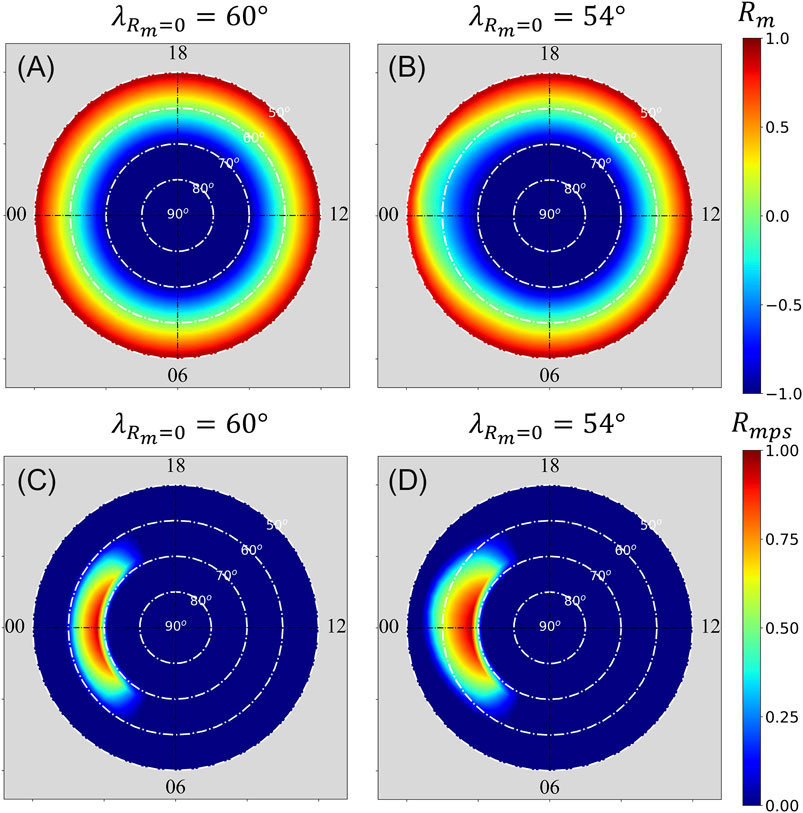
FIGURE 1. Color-level plots of $R_m$ and $R_{m_{PS}}$ with different ${\lambda }_{R_m=0}$, where ${\lambda }_{R_m=0}$ is the magnetic latitude of $R_m=0$ at 23 MLT. Panels (A) and (B) show the distributions of $R_m$ with ${\lambda }_{R_m=0}=60°$ and $54°$, respectively. Panels (C) and (D) show the distributions of $R_{m_{PS}}$ with ${\lambda }_{R_m=0}=60°$ and $54°$, respectively.

Simulation Results

Table 1 lists the simulation parameters used in the 12 simulation cases to be present in this section. The magnetic latitude ${\lambda }_{R_m=0}$ is 54° in Cases 1 and 2 but varies from 54° to 62° in Case 3. We choose ${\lambda }_{R_m=0}=$ 60° in Cases 4a∼6c. To show the importance of the Hall effect in the near-Earth plasma sheet, we set $R_{m_{PS}}=0$ in Cases 2, 4c, 5c, and 6c. We also turn off the conductance enhancement scheme in Cases 4b, 5b, and 6b to show the effect of conductance enhancement in the E-region ionosphere. The initial distributions of the Hall conductance in Cases 1, 2, 3, 6a, 6b, and 6c are similar to the one shown in the KZA′88 model. The initial distribution of the Hall conductance is uniform in Cases 4a∼5c. The uniform conductance is $9 \text{mho}$ in Cases 4a, 4b, and 4c but $1 \text{mho}$ in Cases 5a, 5b, and 5c.

TABLE 1

TABLE 1. Simulation parameters.

Figure 2 shows the simulation results obtained from Case 1 simulation. Case 1 is characterized by time-independent $R_m$ and $R_{m_{PS}}$ distributions with ${\lambda }_{R_m=0}=54°$. Panels (A) and (B) show color-level plots of ${\text{Σ}}_H$ obtained at the 10th step and the 15th step of the simulation, respectively. Panels (C) and (D) show color-level plots of the upward field-aligned current density $J_z$ obtained from the simulation at the 10th step and the 15th step, respectively. Strong field-aligned currents and enhanced Hall conductances appear in the midnight region.

FIGURE 2

FIGURE 2. Simulation results obtained from Case 1 simulation. Case 1 is characterized by time-independent $R_m$ and $R_{m_{PS}}$ distributions with ${\lambda }_{R_m=0}=54°$. Panels (A) and (B) show color-level plots of ${\text{Σ}}_H$ obtained at the 10th step and the 15th step of the simulation, respectively. Panels (C) and (D) show color-level plots of the upward field-aligned current density $J_z$ obtained from the simulation at the 10th step and the 15th step, respectively. Strong field-aligned currents and enhanced Hall conductances appear in the midnight region.

Figure 3 shows color-level plots of (A)${\text{Σ}}_H$ and (B)$J_z$ obtained from the 10th step of the simulation study of Case 2. Case 2 simulation has a time-independent$R_m$ distribution with ${\lambda }_{R_m=0}=54°$. The Hall effect in the thin plasma sheet is turned off in Case 2. A weak upward field-aligned current can be found on the duskside of the polar cap boundary, which can slightly enhance the conductance in that region. The simulation has reached a steady state with very little change on ${\Sigma }_H$ and $J_z$ at the 8th step and beyond. The enhancement of ${\text{Σ}}_H$ on the duskside of the polar cap boundary is less than 10 mho, which is slightly above the maximum of the initial Hall conductance in the diffuse aurora region.

FIGURE 3

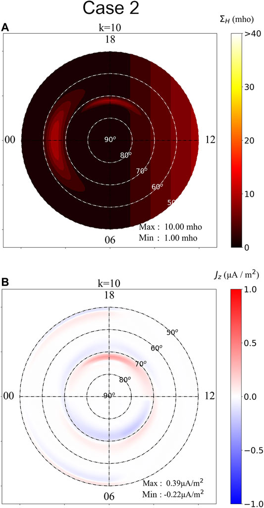
FIGURE 3. Color-level plots of (A)${\text{Σ}}_H$ and (B)$J_z$ obtained from the 10th step of the simulation study of Case 2. Case 2 simulation has a time-independent$R_m$ distribution with ${\lambda }_{R_m=0}=54°$. The Hall effect in the thin plasma sheet is turned off in Case 2. A weak upward field-aligned current can be found at the duskside of the polar cap boundary, which can slightly enhance the conductance in that region.

Figure 4 shows simulation results of Case 3, in the same format as those shown in Figure 2. Case 3 is characterized by time-dependent$R_m$ and $R_{m_{PS}}$ distributions with ${\lambda }_{R_m=0}$ changes from $60°$ to $54°$ and back to $62°.$ Since the distributions of $R_m$ and $R_{m_{PS}}$ are time-dependent, the maximum of the Hall conductance ${\text{Σ}}_H$ and the maximum of the upward field-aligned current density $J_z$ obtained in Case 3 are lower than those shown in Case 1.

FIGURE 4

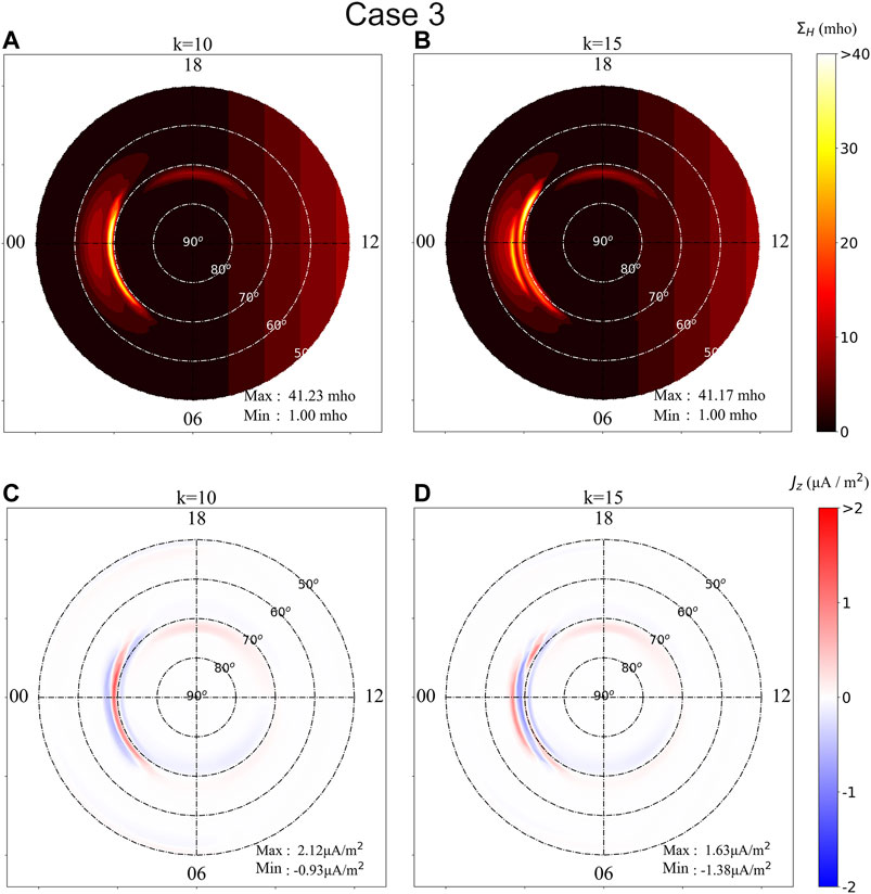
FIGURE 4. Simulation results of Case 3. Panels (A) and (B) show color-level plots of ${\text{Σ}}_H$ obtained at the 10th step and the 15th step of the simulation, respectively. Panels (C) and (D) show color-level plots of the upward field-aligned current density $J_z$ obtained from the simulation at the 10th step and the 15th step, respectively. Case 3 is characterized by time-dependent$R_m$ and $R_{m_{PS}}$ distributions with ${\lambda }_{R_m=0}$ changes from $60°$ to $54°$ and back to $62°.$ Since the distributions of $R_m$ and $R_{m_{PS}}$ are time dependent, the maximum of the Hall conductance ${\text{Σ}}_H$ and the maximum of the upward field-aligned current density $J_z$ obtained in Case 3 are lower than those shown in Case 1.

Figure 5 shows the time evolution of (A)${\left(J_z\right)}_{\max }$, (B)${\left(J_z\right)}_{\min }$, and (C)${\left({\Sigma }_H\right)}_{\max }$ obtained from the simulations of Case 1 (the solid curves), Case 2 (the dashed curves), and Case 3 (the dotted curves). ${\left(J_z\right)}_{\max }$ denotes the maximum upward field-aligned current density in the entire simulation domain obtained at the kth step of the simulation. The absolute value of ${\left(J_z\right)}_{\min }$ denotes the maximum of the downward field-aligned current density in the entire simulation domain obtained at the kth step of the simulation. ${\left({\Sigma }_H\right)}_{\max }$ denotes the maximum Hall conductance in the entire simulation domain obtained at the kth step of the simulation. The time evolution of ${\left(J_z\right)}_{\max }$ is similar to the time evolution of ${\left({\Sigma }_H\right)}_{\max }$ due to the choice of the conductance enhancement scheme discussed in Eqs 26, 27. The Hall effects in the magnetotail lead to a similar growth phase ($5<k<11$) in Case 1 and Case 3. The time-independent distributions of $R_m$ and $R_{m_{PS}}$ used in the Case 1 simulation yield a second growth phase at $k>17$ in the Case 1 simulation. Ignoring the Hall effects in the magnetotail, the three dashed curves of Case 2 show very little enhancement on the field-aligned current density and the Hall conductance.

FIGURE 5

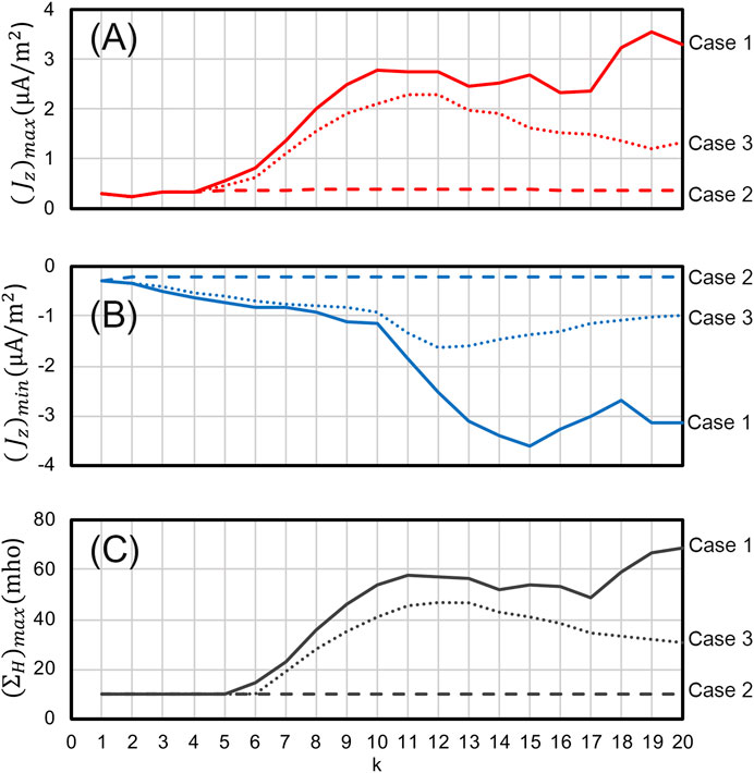
FIGURE 5. The time evolution of (A)${\left(J_z\right)}_{\max },$(B)${\left(J_z\right)}_{\min },$ and (C)${\left({\Sigma }_H\right)}_{\max }$ obtained from the simulations of Case 1 (the solid curves), Case 2 (the dashed curves), and Case 3 (the dotted curves).

Figure 6 shows the time evolution of (A)${\left(J_z\right)}_{\max }$, (B)${\left(J_z\right)}_{\min }$, and (C)${\left({\Sigma }_H\right)}_{\max }$ obtained from the simulations of Case 4a (the solid curves), Case 4b (the dashed curves), and Case 4c (the dotted curves). Simulation Cases 4a, 4b, and 4c are characterized by uniform high conductances at the beginning of the simulations. The initial Hall conductance is $9 \text{mho}\text{.}$ The conductance enhancement scheme is turned off in Case 4b. Without gradient on the ionospheric conductances, the field-aligned current density obtained in Case 4b is lower than it in Case 4a. The plasma sheet Hall effect is turned off in Case 4c. Without the Hall effect in the plasma sheet, very little enhancement on the field-aligned current density and the Hall conductance can be seen in the simulation of Case 4c.

FIGURE 6

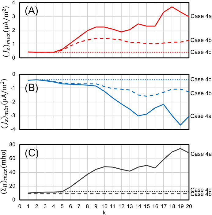
FIGURE 6. The time evolution of (A)${\left(J_z\right)}_{\max },$(B)${\left(J_z\right)}_{\min },$ and (C)${\left({\Sigma }_H\right)}_{\max }$ obtained from the simulations of Case 4a (the solid curves), Case 4b (the dashed curves), and Case 4c (the dotted curves). Simulation Cases 4a, 4b, and 4c are characterized by uniform high conductances $\left({\Sigma }_H=9 \text{mho}\right)$ at the beginning of the simulations. The conductance enhancement scheme is turned off in Case 4b. The plasma sheet Hall effect is turned off in Case 4c.

Figure 7 shows the time evolution of (A)${\left(J_z\right)}_{\max }$, (B)${\left(J_z\right)}_{\min }$, and (C)${\left({\Sigma }_H\right)}_{\max }$ obtained from the simulations of Case 5a (the solid curves), Case 5b (the dashed curves), and Case 5c (the dotted curves). Simulation Cases 5a, 5b, and 5c are characterized by uniform low conductances at the beginning of the simulations. The initial Hall conductance is $1 \text{mho}$. The conductance enhancement scheme is turned off in the simulation study of Case 5b. The plasma sheet Hall effect is turned off in the simulation study of Case 5c. Without gradient on the ionospheric conductances, the field-aligned current density obtained in Case 5b shows a minimal growth rate. Without considering the Hall effect in the plasma sheet, very little enhancement on the field-aligned current density and the Hall conductance can be found in the simulation study of Case 5c.

FIGURE 7

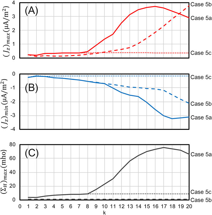
FIGURE 7. The time evolution of (A)${\left(J_z\right)}_{\max },$(B)${\left(J_z\right)}_{\min },$ and (C)${\left({\Sigma }_H\right)}_{\max }$ obtained from the simulations of Case 5a (the solid curves), Case 5b (the dashed curves), and Case 5c (the dotted curves). Simulation Cases 5a, 5b, and 5c are characterized by uniform low conductances (${\text{Σ}}_H=1 \text{mho}$) at the beginning of the simulations. The conductance enhancement scheme is turned off in the simulation study of Case 5b. The plasma sheet Hall effect is turned off in the simulation study of Case 5c.

Let us compare the simulation results of Case 4a and Case 5a shown in Figures 6, 7. The ${\left(J_z\right)}_{\max }$ curve obtained in Case 4a shows a short lag phase followed by a growth phase from the 4th step to the 10th step, but with a relatively low saturation level ${\left(J_z\right)}_{\max }\approx 2.3 \text{μA}/m^2$. The ${\left(J_z\right)}_{\max }$ curve obtained in Case 5a shows a prolonged lag phase followed by a growth phase from the 8th step to the 16th step, but with a relatively high saturation level at ${\left(J_z\right)}_{\max }\approx 3.8 \text{μA}/m^2$. The ${\left(J_z\right)}_{\max }$ curve obtained in the simulation study of Case 4a shows a second peak at the 14th step and a third peak at the 18th step. The highest upward field-aligned current density can be found at the 18th step with ${\left(J_z\right)}_{\max }\approx 3.8 \text{μA}/m^2$. The differences between the ${\left(J_z\right)}_{\max }$ curves shown in Case 4a and Case 4b are less significant than the differences between the ${\left(J_z\right)}_{\max }$ curves shown in Case 5a and Case 5b

Figure 8 shows the time evolution of (A)${\left(J_z\right)}_{\max },$(B)${\left(J_z\right)}_{\min },$ and (C)${\left({\Sigma }_H\right)}_{\max }$ obtained from Case 6a (the solid curves), Case 6b (the dashed curves), and Case 6c (the dotted curves) simulations. The initial distributions of the conductances of the three cases are nonuniform and are similar to the one used in Cases 1–3. The conductance enhancement scheme in the ionosphere is turned off in the simulation study of Case 6b. The plasma sheet Hall effect is turned off in the simulation study of Case 6c. Again, without the Hall effect in the plasma sheet, very little enhancement on the field-aligned current density and the Hall conductance can be found in the simulation study of Case 6c. But the differences between the ${\left(J_z\right)}_{\max }$ curves obtained in Case 6a and Case 6b are relatively small due to the preexisting nonuniform conductance in the diffuse aurora region. The ${\left(J_z\right)}_{\max }$ curves of Case 6a show a growth phase from the 6th step to the 12th step and with a saturation level at ${\left(J_z\right)}_{\max }\approx 2 \text{μA}/m^2$.

FIGURE 8

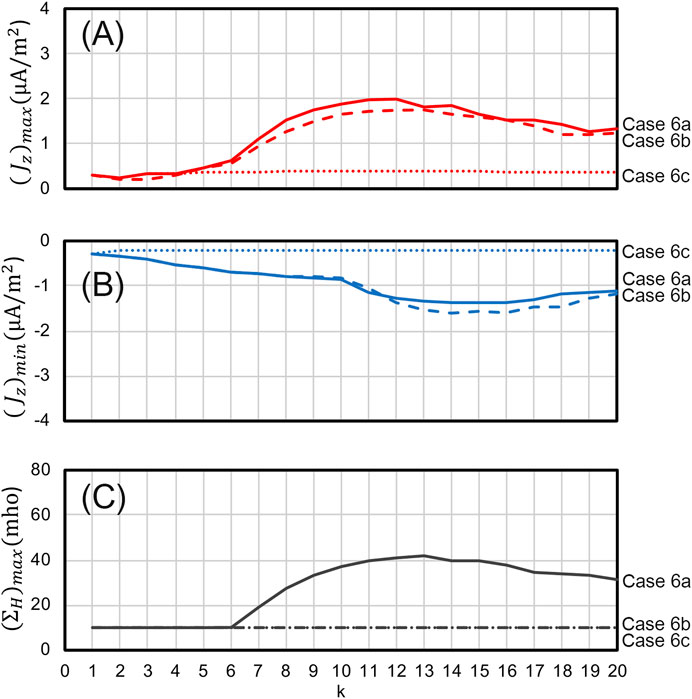
FIGURE 8. The time evolution of the (A)${\left(J_z\right)}_{\max }$, (B)${\left(J_z\right)}_{\min }$, and (C)${\left({\Sigma }_H\right)}_{\max }$ obtained from Case 6a (the solid curves), Case 6b (the dashed curves), and Case 6c (the dotted curves) simulations. The initial distributions of the conductances of the three cases are nonuniform and are similar to the one used in Cases 1–3. The conductance enhancement scheme in the ionosphere is turned off in the simulation study of Case 6b. The plasma sheet Hall effect is turned off in the simulation study of case 6c.

Summary and Discussion

In summary, we have constructed a new M-I coupling model modified from the M-I coupling model proposed by Kan et al. (1988). We adjust the magnetospheric boundary conditions by including the Hall effects in the thin current sheet. As a result, multiple brightening auroral arcs appear in the midnight region and gradually move poleward. This region is characterized by $-1\mathrm{\lesssim }{R}_m<0$ and $0<R_{m_{PS}}\le 1$.

A steady midnight auroral arc has also been found in the simulation study by Kan and Sun (1996). The formation of the midnight arc results from an enhanced localized convection electric field added in their simulation. A localized convection electric field has also been considered in the early simulation studies (e.g., Kan et al., 1988), but no midnight aurora arc can be found. These results indicate that only a particular type of convection electric field can result in a midnight aurora arc.

The enhancement of ionospheric conductances by the upward field-aligned currents can increase the nonuniformity of the ionospheric conductances. The nonuniform Hall effect in the plasma sheet can result in the nonuniform rotation of the electric field in the plasma sheet. The nonuniform rotation of the electric field in the plasma sheet obtained in this study and the localized convection electric field proposed by Kan and Sun (1996) can result in upward and downward field-aligned currents in the midnight region.

The simple M-I coupling model provides much helpful information for 3-dimensional global simulations of magnetospheric substorms. The simulation results shown in Figures 6–8 in the last section indicate that the high conductance in the ionosphere can speed up the growth phase of a substorm event but result in a relatively weak upward field-aligned current in the auroral arc. On the other hand, a substorm event with low preexisting conductance in the ionospheric boundary requires a longer time to complete the growth phase. Still, it can build up a much stronger upward field-aligned current in the auroral arc. The simulation results discussed in Figures 6–8 also indicate that including the conductance enhancement processes on the ionosphere boundary can increase the field-aligned current intensity in a global simulation of the magnetospheric substorm. The Hall effect in the thin current sheet should also be included in future simulation studies of magnetospheric substorms.

Data Availability Statement

The original contributions presented in the study are included in the article/Supplementary Material; further inquiries can be directed to the corresponding author.

Author Contributions

All authors listed have made a substantial, direct, and intellectual contribution to the work and approved it for publication.

Funding

This work was supported by the MOST grants 107-2111-M-008-007 and 108-2111-M-008-019 to the National Central University.

Conflict of Interest

The authors declare that the research was conducted in the absence of any commercial or financial relationships that could be construed as a potential conflict of interest.

Acknowledgments

This work is a part of the master degree thesis work by PW. We would like to thank L. Zhu for providing his Ph.D. Thesis to LL. for references.

References

Akasofu, S.-I. (1964). The Development of the Auroral Substorm. Planet. Space Sci. 12, 273–282. doi:10.1016/0032-0633(64)90151-5

CrossRef Full Text | Google Scholar

Bunescu, C., Vogt, J., Marghitu, O., and Blagau, A. (2019). Multiscale Estimation of the Field-Aligned Current Density. Ann. Geophys. 37, 347–373. doi:10.5194/angeo-37-347-2019

CrossRef Full Text | Google Scholar

Cheng, C. Z., and Lui, A. T. Y. (1998). Kinetic Ballooning Instability for Substorm Onset and Current Disruption Observed by AMPTE/CCE. Geophys. Res. Lett. 25, 4091–4094. doi:10.1029/1998GL900093

CrossRef Full Text | Google Scholar

Coppi, B., Laval, G., and Pellat, R. (1966). Dynamics of the Geomagnetic Tail. Phys. Rev. Lett. 16, 1207–1210. doi:10.1103/PhysRevLett.16.1207

CrossRef Full Text | Google Scholar

Fridman, M., and Lemaire, J. (1980). Relationship between Auroral Electrons Fluxes and Field Aligned Electric Potential Difference. J. Geophys. Res. 85 (A2), 664–670. doi:10.1029/JA085iA02p00664

CrossRef Full Text | Google Scholar

Furth, H. P., Killeen, J., and Rosenbluth, M. N. (1963). Finite-Resistivity Instabilities of a Sheet Pinch. Phys. Fluids 6, 459. doi:10.1063/1.1706761

CrossRef Full Text | Google Scholar

Iijima, T., and Potemra, T. A. (1976). The Amplitude Distribution of Field-Aligned Currents at Northern High Latitudes Observed by Triad. J. Geophys. Res. 81 (13), 2165–2174. doi:10.1029/JA081i013p02165

CrossRef Full Text | Google Scholar

Kamide, Y., and Horwitz, J. L. (1978). Chatanika Radar Observations of Ionospheric and Field-Aligned Currents. J. Geophys. Res. 83 (A3), 1063–1070. doi:10.1029/JA083iA03p01063

CrossRef Full Text | Google Scholar

Kamide, Y. (1982). The Relationship between Field-Aligned Currents and the Auroral Electrojets: A Review. Space Sci. Rev. 31, 127–243. doi:10.1007/bf00215281

CrossRef Full Text | Google Scholar

Kan, J. R., and Kamide, Y. (1985). Electrodynamics of the Westward Traveling Surge. J. Geophys. Res. 90 (A8), 7615–7619. doi:10.1029/JA090iA08p07615

CrossRef Full Text | Google Scholar

Kan, J. R., and Sun, W. (1985). Simulation of the Westward Traveling Surge and Pi 2 Pulsations during Substorms. J. Geophys. Res. 90 (A11), 10911–10922. doi:10.1029/JA090iA11p10911

CrossRef Full Text | Google Scholar

Kan, J. R., and Sun, W. (1996). Substorm Expansion Phase Caused by an Intense Localized Convection Imposed on the Ionosphere. J. Geophys. Res. 101 (A12), 27271–27281. doi:10.1029/96JA02426

CrossRef Full Text | Google Scholar

Kan, J. R., Zhu, L., and Akasofu, S.-I. (1988). A Theory of Substorms: Onset and Subsidence. J. Geophys. Res. 93 (A6), 5624–5640. doi:10.1029/JA093iA06p05624

CrossRef Full Text | Google Scholar

Kaufmann, R. L. (1987). Substorm Currents: Growth Phase and Onset. J. Geophys. Res. 92 (A7), 7471–7486. doi:10.1029/JA092iA07p07471

CrossRef Full Text | Google Scholar

Knight, S. (1973). Parallel Electric fields. Planet. Space Sci. 21, 741–750. doi:10.1016/0032-0633(73)90093-7

CrossRef Full Text | Google Scholar

Lui, A. T. Y., Yoon, P. H., and Chang, C.-L. (1993). Quasi-linear Analysis of Ion Weibel Instability in the Earth's Neutral Sheet. J. Geophys. Res. 98 (A1), 153–163. doi:10.1029/92JA02034

CrossRef Full Text | Google Scholar

Lui, A. T. Y., Yoon, P. H., Mok, C., and Ryu, C.-M. (2008). Inverse cascade Feature in Current Disruption. J. Geophys. Res. 113, a–n. doi:10.1029/2008JA013521

CrossRef Full Text | Google Scholar

Lyu, L. H., and Chen, M. Q. (2000). A Kinetic M-I Coupling Model with Unloading Instability at Onset of Substorm. in Proc. 5th International Conference on Substorms, St. Petersburg, Russia, 315–318. 16-20 May 2000, ESA SP-443.

Google Scholar

McPherron, R. L. (1972). Substorm Related Changes in the Geomagnetic Tail: the Growth Phase. Planet. Space Sci. 20, 1521–1539. doi:10.1016/0032-0633(72)90054-2

CrossRef Full Text | Google Scholar

Miura, A., and Sato, T. (1981). Global Simulation of Auroral Arcs, in Physics of Auroral Arc Formation, ed. by S.‐I. Akasofu, and J. Kan, pp. 321–332. Washington, DC: Geophysical Monograph Series, Volume 25. doi:10.1029/GM025p0321

CrossRef Full Text | Google Scholar

Miura, A., and Sato, T. (1980). Numerical Simulation of Global Formation of Auroral Arcs. J. Geophys. Res. 85 (A1), 73–91. doi:10.1029/JA085iA01p00073

CrossRef Full Text | Google Scholar

Ohtani, S., Takahashi, K., Zanetti, L. J., Potemra, T. A., McEntire, R. W., and Iijima, T. (1992). Initial Signatures of Magnetic Field and Energetic Particle Fluxes at Tail Reconfiguration: Explosive Growth Phase. J. Geophys. Res. 97 (A12), 19311–19324. doi:10.1029/92JA01832

CrossRef Full Text | Google Scholar

Pitout, F., Marchaudon, A., Blelly, P. L., Bai, X., Forme, F., Buchert, S. C., et al. (2015). Swarm and ESR Observations of the Ionospheric Response to a Field‐aligned Current System in the High‐latitude Midnight Sector. Geophys. Res. Lett. 42, 4270–4279. doi:10.1002/2015GL064231

CrossRef Full Text | Google Scholar

Podgorny, I. M., Podgorny, A. I., Minami, S., and Rana, R. (2003). The Mechanism of Energy Release and Field-Aligned Current Generation during Substorms and Solar Flares. Adv. Polar Upper Atmos. Res. 17, 77–83.

Google Scholar

Robinson, R. M., Vondrak, R. R., and Potemra, T. A. (1985). Auroral Zone Conductivities within the Field-Aligned Current Sheets. J. Geophys. Res. 90 (A10), 9688–9696. doi:10.1029/JA090iA10p09688

CrossRef Full Text | Google Scholar

Roux, A., Perraut, S., Robert, P., Morane, A., Pedersen, A., Korth, A., et al. (1991). Plasma Sheet Instability Related to the Westward Traveling Surge. J. Geophys. Res. 96 (A10), 17697–17714. doi:10.1029/91JA01106

CrossRef Full Text | Google Scholar

Schindler, K. (1974). A Theory of the Substorm Mechanism. J. Geophys. Res. 79 (19), 2803–2810. doi:10.1029/JA079i019p02803

CrossRef Full Text | Google Scholar

Walén, C. (1944). On the Theory of Sunspots. Ark. Mat. Astron. Fys. 30A, 15.

Google Scholar

Wing, S., and Johnson, J. R. (2015). Theory and Observations of Upward Field-Aligned Currents at the Magnetopause Boundary Layer. Geophys. Res. Lett. 42, 9149–9155. doi:10.1002/2015GL065464

PubMed Abstract | CrossRef Full Text | Google Scholar