 Anna Malanushenko
 Natasha Flyer2
 Sarah Gibson
- 1High Altitude Observatory, National Center for Atmospheric Research, Boulder, CO, United States
- 2Department of Applied Mathematics, University of Colorado, Boulder, CO, United States
In this paper, we explore the potential of neural networks for making space weather predictions based on near-Sun observations. Our second goal is to determine the extent to which coronal polarimetric observations of erupting structures near the Sun encode sufficient information to predict the impact these structures will have on Earth. In particular, we focus on predicting the maximal southward component of the magnetic field (“−Bz”) inside an interplanetary coronal mass ejection (ICME) as it impacts the Earth. We use Gibson & Low (G&L) self-similarly expanding flux rope model (Gibson and Low, 1998) as a first test for the project, which allows to consider CMEs with varying location, orientation, size, and morphology. We vary 5 parameters of the model to alter these CME properties, and generate a large database of synthetic CMEs (over 36k synthetic events). For each model CME, we synthesize near-Sun observations, as seen from an observer in quadrature (assuming the CME is directed earthwards), of either three components of the vector magnetic field, (Bx, By, Bz) (“Experiment 1”), or of synthetic Stokes images, (L/I, Az, V/I) (“Experiment 2”). We then allow the flux rope to expand and record max{−Bz} as the ICME passes 1AU. We further conduct two separate machine learning experiments and develop two different regression-based deep convolutional neural networks (CNNs) to predict max{−Bz} based on these two kinds of the near-Sun input data. Experiment 1 is a test which we do as a proof of concept, to see if a 3-channel CNN (hereafter CNN1), similar to those used in RGB image recognition, can reproduce the results of the self-similar (i.e., scale-invariant) expansion of the G&L model. Experiment 2 is less trivial, as Stokes vector is not linearly related to B, and the line-of-sight integration in the optically thin corona presents additional difficulties for interpreting the signal. This second CNN (hereafter CNN2), although resembling CNN1 in Experiment 1, will have a different number of layers and set of hyperparameters due to a much more complicated mapping between the input and output data. We find that, given three components of B, CNN1 can predict max{−Bz} with 97% accuracy, and for three components of the Stokes vector as input, CNN2 can predict max{−Bz} with 95%, both measured in the relative root square error.
1. Introduction
Geomagnetic storms are powerful disturbances in Earth's magnetosphere, which become increasingly more important as our technologies develop. The technological progress increases the quality of our lives and our understanding of world around us, yet it renders us increasingly more dependent on electricity, telecommunications, satellites, and air transportation. These are some of the areas most impacted by the geomagnetic storms (National Research Council, 2008; Eastwood et al., 2017). While the well-known Carrington event has resulted, in 1859, in some damage to telegraph lines and spectacular auroras seen as far as Hawaii (Cliver and Dietrich, 2013), an event of a similar magnitude happening today would be devastating for the modern civilization (National Research Council, 2008; Baker, 2013).
The mitigation efforts depend on our ability to predict the strength and the duration of a storm before it happens, in order to take costly, yet necessary protective measures. These include redirecting air traffic, taking measures to protect the power grid, or preparing for inevitable disturbances in telecommunications (e.g., Knipp and Gannon, 2019).
Geomagnetic storms are often caused by the collision of Earth's magnetic field with clouds of magnetized plasma, which are typically of solar origin. The strength of a storm crucially depends on the strength of the magnetic field in the cloud, and also on its orientation with respect to the Earth's own magnetic field. A large southward component of the magnetic field (hereafter Bz < 0) will result in stronger storms than if the field had a comparable northward component (Bz > 0). These clouds are associated with coronal mass ejections (CMEs), the eruptive phenomena observed on the Sun (Webb and Howard, 2012).
The ability to predict the strength of geomagnetic storms, consequently, relies on our ability to detect a CME as it departs the Sun, to predict whether Earth will lie on its way, and to predict its properties at the moment of its encounter with Earth (Kilpua et al., 2019). Typically, after a CME is detected, simulations of its propagation through interplanetary space are needed to predict its further evolution as an interplanetary CME, or ICME (e.g., Arge et al., 2004; Manchester et al., 2017).
CMEs are magnetic in nature (e.g., Chen, 2011; Bak-Stȩślicka et al., 2013; Forland et al., 2013); hence, near-Sun observations sensitive to the strength of a magnetic field are needed to determine the properties of a particular erupting structure. To obtain magnetic information, measurements of spectral line profiles of polarized light must be obtained. Unfortunately, many existing observations of magnetic field regard only the solar photosphere and chromosphere, while the CMEs are observed in the solar corona. As the corona is significantly dimmer than the solar surface in visible/infrared light, observations of CMEs in these wavelengths require a coronagraph to occult the disk of the Sun.
The spectropolarimetric measurements generally include four Stokes parameters (I, Q, U, V) (unpolarized intensity, intensity in two directions of a linear, and intensity of a circular polarization, respectively) at several locations along a spectral line. These carry information about the magnetic field in the emitting plasma. In solar photospheric observations (e.g., Schou et al., 2012), the Stokes vector can be inverted (e.g., Ruiz Cobo and del Toro Iniesta, 1992) to obtain components of the magnetic field, (Bx, By, Bz), at the solar photosphere. But in coronal observations, the inversion is greatly complicated by the fact that corona is optically thin; the observed signal is integrated not over a relatively small range of heights, like in photospheric observations, but over hundreds of megameters. Nevertheless, although the direct inversion of Stokes data in the corona is complicated, we often observe clear signatures of magnetic structures, consistent with existing models of CMEs, in coronal spectropolarimetric measurements (Gibson, 2015). This introduces the possibility of using such observations to diagnose the magnetic field at the core of the CME at its origins at the Sun. We note, however, that because the observations are at the limb of the Sun, the CME being diagnosed would be aimed at a right angle to the observer. Ideally, one would want to make the limb observations from an instrument placed in quadrature with respect to the Sun-Earth line. Such an instrument does not yet exist but the usefulness of it can be explored with the use of synthesized observations for example using forward modeling (Gibson et al., 2016).
At least two factors will affect the ability of coronal spectropolarimetric measurements to provide a good predictor of geomagnetic storms. First, since the corona is optically thin, spectropolarimetric measurements of linearly and circularly polarized light diagnose magnetic field strength and geometry in a weighted line-of-sight integral that must be inverted to obtain magnetic field. Second, evolution between the Sun and Earth will change the erupting structure in ways that will not be captured in the measurement obtained in its early stages in the solar atmosphere. The purpose of this work is to investigate how good of a predictor such coronal signatures are for the strength of the associated geomagnetic storm at the Earth if machine learning algorithms are used, bypassing the need for inversions of line-of-sight integrated spectropolarimetric signals, and also bypassing computationally expensive simulations of how ICMEs propagate through the interplanetary space.
In this paper, the first factor is examined by the following two machine learning experiments. A particular model of a CME called G&L (Gibson and Low, 1998), described in section 2, is used for generating input and output data in both experiments. The total of 36,288 different configurations of magnetic flux ropes are generated over the 5D space of parameters that control morphology, shape, and position. We then generate two kinds of synthetic near-Sun input data, at the time prior to eruption: either three components of the magnetic field (Bx, By, Bz) on a slice at the central meridian (“Experiment 1”), or the Stokes linear and circular polarization normalized by intensity (L/I, Az, V/I), integrated along the line of sight (“Experiment 2”). (Note that and contain the same information as Q and U normalized by I.) We also generate synthetic 1AU output data, common for both experiments: as the flux rope expands, we record the maximal southward component of the magnetic field (hereafter max{−Bz}) within the ICME flux rope as it impacts the Earth and drives the storm.
In Experiment 1, a binary classifier using fully connected feedforward neural network (FNN), is constructed to determine whether the ICME is launched in such a direction as to impact Earth (a “storm” or a “no storm” prediction), based on an input image of one of the three magnetic field components. We further refer to this network as FNN1. For those ICMEs classified as a “storm,” we further construct a 3-channel convolutional neural network (CNN), which inputs all three components of the magnetic field, and has the objective to predict max{−Bz} at 1AU. We further refer to this network as CNN1.
Based on the optimistic results from CNN1, we perform a separate Experiment 2 with synthetic spectropolarimetric data. As these data are of a different nature, we create a new set of neural networks, independent from Experiment 1, but with similar type architectures. For this experiment, the input data are pre-eruption near-Sun coronal spectropolarimetric measurements. Another binary classifier, hereafter FNN2, uses spectropolarimetric data in different combinations (only circularly polarized light, only linearly, and all three components), to make, as in Experiment 1, a “storm” / “no storm” prediction. Next, a new CNN, hereafter CNN2, is constructed in the similar fashion as in Experiment 1. It is again run on those events classified as a “storm,” and uses all three components of the Stokes data, to predict max{−Bz}. In this way, we take into account the line of sight weighting of the observable quantity, and also consider the different diagnostic potential of circularly vs. linearly polarized light.
The paper is structured as follows. In section 2, we describe the G&L model used for synthesizing the data and describe in detail the parameters which were varied. In section 3, we describe the synthetic input and output data, and the architecture of neural networks which we constructed for each experiment. In section 4, we report the results of each experiment and demonstrate that in both cases of input data, both networks could make successful predictions. Finally, in section 5 we discuss the implication of the results and outline the path for future development of this machine learning application.
2. Analytic CME Model Used for Training and Testing CNN
We use a CME model called G&L (Gibson and Low, 1998) to build a database of erupting flux ropes with varying characteristics. G&L is an analytical 3D magnetohydrodynamic (MHD) model with a spheromak-like magnetic flux rope1 embedded in a bipolar background magnetic field and radially symmetric background hydrostatic atmosphere. The bubble which contains the flux rope expands self-similarly with time, modeling the propagation of a CME through the interplanetary space. While the self-similar expansion is a rather idealized model of CME propagation, the current work is meant to prepare the framework for the next step of the project. In the next step, we will keep the structure of the project, but instead of a self-similar expansion, will use results from more realistic MHD simulations (Merkin et al., 2016) of ICME propagation, which will nonetheless use the same G&L flux ropes as initial condition. This is further explained in section 5.
A given G&L solution depends on a large number of analytical and empirical parameters (Gibson et al., 2016). For the purpose of this study, we choose to vary 5 parameters most relevant to the shape, topology, and position of the flux rope These parameters are: height of the front of the CME, its angular width, the “topology” parameter, the rotation about the Sun-to-1-AU line that passes through the center of the CME, and latitude from which the CME is launched. The further sections describe the parameters in detail. Several of the solutions from the database are shown in Figure 1. The ranges of each parameter are further listed in Table 1.
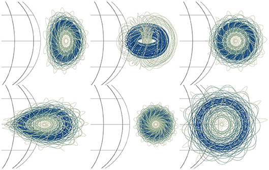
Figure 1. Examples of various initial G&L configurations. Blue and green lines are magnetic field lines sampling the magnetic structure of the G&L spheromak, shown here with different combinations of parameters for angular size, topology, orientation. The solar surface is shown in thin black lines for reference.
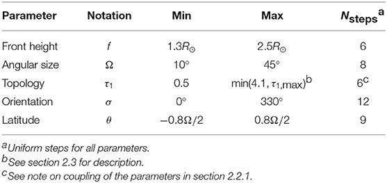
Table 1. Ranges of the G&L parameters.
2.1. Size and Initial Height Parameters
The original Gibson and Low (1998) defined the geometry of the embedded spheromak through the following three parameters. The bubble of radius r0 was located at a distance x0 from the origin (Sun's center), and the subsequent stretching transformation r → r + a was applied in spherical coordinates, where a = const is a stretching parameter, constant for the entire domain. Further, in the FORWARD suite which we use for the calculations (Gibson et al., 2016), r0 and x0 were replaced by two parameters which are more directly related to observations: the angular size of the bubble Ω, defined as tan(Ω/2) = r0/x0, and the height of the front of the bubble f = x0 + r0 − a. By definition in the model, all points for which r ≤ a are fixed at the origin (r = 0) and stay in the origin during the self-similar expansion. The resulting solution has a spherical bubble for a = 0, teardrop-shaped bubble for a > 0, and umbrella-shaped bubble for a < 0, as shown in Figure 2.
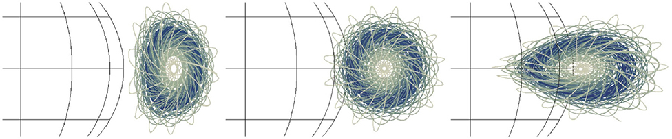
Figure 2. Flux rope which correspond to different values of the stretching parameter a. Left: a < 0, middle: a = 0, right: a > 0. The exact values are a = −0.5R⊙, a = 0R⊙, and a = 0.8R⊙, respectively. The values of the other parameters used in this illustration are: f = 1.95R⊙, Ω = 50°, σ = 90°, and θ = 0°.
2.2. Topology/Stretching Parameter
In this study, we introduce a new parameter to replace a, which is more directly related to the topology of the over-the-limb portion of the flux rope: τ1. Consider the coordinates shown in Figure 3, with ẑ normal to the plane of the solar equator, and the flux rope propagating radially along axis along the Sun-Earth line.
Figure 3. The coordinates used in the model. The Sun-Earth line is along axis. The dotted lines show the location of the “key” points along axis, from left to right: back of the bubble A, back end of the minor axis B, major axis C, front end of the minor axis D, and front of the bubble E.
We notice that there are several geometrically special points along axis, shown in Figure 3. E.g., consider point A which is the back end of the bubble (or closest to the origin). If the value of a is such that xA > R⊙ (or x0 − r0 − a > R⊙)2, then the entire spheromak is above solar surface (called the photosphere), and field lines are generally infinite, wrapping infinitely about the core of the spheromak. If a is such that xA < R⊙, but xB > R⊙, then some portion of the bubble will be under the solar surface prior to “eruption”; for the purpose of the study we keep track of this portion during the self-similar expansion and do not include this portion in the calculations of the strength of geomagnetic storm. The coronal portion of the bubble will contain spheromak-like field lines, as well as field lines which begin and end at the solar surface—the overall configuration will appear as a spheromak suspended in sheared-arcade of field lines. Similarly, xB < R⊙ < xC would create an apparent classical flux-rope configuration (e.g., Gold and Hoyle, 1960; Fan and Gibson, 2003), in the sense that both footpoints of field lines are anchored at the photosphere, but the field lines wrap around a common arch-like axis and have dips which potentially could support cool prominence material (Fan and Liu, 2019). Further, xC < R⊙ < xE would mean that all field lines above the r = R⊙ surface are arches and the overall coronal portion would appear to be a sheared arcade.
For the purpose of this study, we ignore the portion of the flux rope which is underneath the solar surface prior to eruption (see section 3 for detail on how is this implemented in the output data.) The parameter , where k = tan(Ω/2) = r0/x0, is an empirical dimensionless parameter related to how many special points are above the photosphere. For example, τ1 < 0 means that all special points are below r = R⊙, 0 < τ1 < 1 means one of these points is above r = R⊙, etc, and τ1 > 4 means the entire bubble is above the surface3. Note that τ1 is also related to the shape of the bubble: decreasing τ1 while keeping constant f and Ω will make the bubble more teardrop-stretched. For example, Figure 2 shows, from left to right, solutions for τ1 ≈ 4.1, 3.2, 2.2, with 5, 4, and 3 special points above the surface respectively. Varying τ1 allows us to sample qualitatively different magnetic configurations, including, for example, the classical flux rope (2 ≤ τ1 ≤ 3) and the toroidal spheromak (τ1 ≥ 4). Observational evidence for different topologies including simple flux ropes (Bak-Stȩślicka et al., 2013) and spheromaks (Dove et al., 2011) have been found in polarimetric observations of coronal cavities, known to be cavities, known to be precursors of CMEs (Gibson, 2015).
Lastly, we notice that the value of τ1 for which a = 0 and the bubble is spherical is τ1, max = 2(f−1)(k+1)/(kf). We do not use solutions for a < 0, or equivalently, of τ1 > τ1,max, as they are deemed unphysical4. In addition, choices of τ1 > 4 result in a flux rope bubble that hovers above the photosphere at t = 0. Coronal cavity CME precursors tend to maintain some measure of contact with the photosphere—although, for highly stretched, teardrop-shaped bubbles some hovering is observed (e.g., Forland et al., 2013). Therefore, we cap the range of τ1 by the smallest of two values: τ1 < min(4.1, τ1, max) ensuring that none of the bubbles are in either the unphysical a < 0 regime, nor too far from the photosphere before the eruption. Note that this implies that the parameter space is not uniform in τ1: for each pair of (f, Ω), the range of τ1 is calculated independently, and uniform steps in τ1 are taken in that range.
2.2.1. Coupling of the Parameters
The three parameters described above, f, Ω, and τ1, are secondary in the sense that they have been introduced and can be expressed through the primary parameters which define properties of the spheromak in the G&L model, x0, r0, and a:
However, the secondary parameters can be more easily related to the observed properties of CMEs (e.g., x0 is the location of the spheromak's center before the stretching has been applied, and the resulting position of the bubble would in general be different.) To make our study more useful for future work in CME predictions, we invert the system (1) and express primary parameters through the secondary ones:
We then vary the secondary parameters, in the ranges shown in Table 1, calculate the primary parameters through (2), and use these as the input to the G&L model.
2.3. Orientation and Latitude Parameters
The orientation of the spheromak's core, with respect to the Earth's North, is an important parameter for determining the strength of the geomagnetic storm. We vary parameter σ that defines rotation of the bubble about the radial direction. Figure 4 shows several solutions with varying σ.
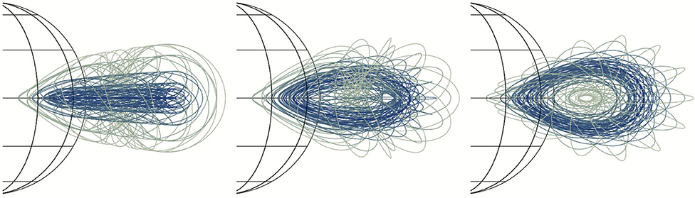
Figure 4. Flux ropes rotated by a different amount σ about the direction of propagation (in this case, ). From left to right: σ = 0°, 42.4°, 84.7°.
The last parameter that we vary is the starting latitude of the CME, θ. Since the subsequent expansion is self-similar, the direction of propagation is radial and a CME remains within the same solid angle at all times. The Sun-Earth line is along , so CMEs launched at θ > Ω/2 with respect to the equator will miss Earth completely, and θ ≈ Ω/2 will have a vanishingly small effect on Earth. As we show later, the CNN is taught to determine which CMEs will result in a “storm,” and which will result in “no storm” at the Earth. We adjust σ range so that about 82% of all CMEs result in a “storm” at the Earth, in the sense of .
3. Neural Networks: Data and Architectures
Two experiments are conducted, each with two neural networks (NNs)—a feedforward fully connected neural network (FNN) and a 3 channel convolutional network (CNN) that can also accept 1 or 2 channels of data. For each experiment, these NN are different. Hence, there are a total of 4 separate NNs. The FNN acts as a binary classifier, determining whether there is a “storm”5 or a “no storm.” Both CNN1 in Experiment 1 and CNN2 in Experiment 2 perform a non-linear regression to estimate max{−Bz} inside the flux rope as it impacts Earth and drives the storm, for those events classified as “storms.” The big difference between the experiments is 1) the input data and 2) the NN architectures, due to a change in the characteristics of the input data. Both will be discussed in the following subsections. We refer the readers who are not familiar with FNN and CNN to textbooks and overview articles on the topic (e.g., Svozil et al., 1997; Goodfellow et al., 2016; Yamashita et al., 2018). All code was programmed in MATLAB package “Deep Learning Toolbox” (The MathWorks, 2019).
For both experiments, the output data are the same—the maximal negative (southward) amplitude of the Bz component in the flux rope at 1AU: max{−Bz(t)}, which serves as a proxy for the strength of the geomagnetic storm. It is calculated as follows. The flux rope was allowed to expand self-similarly, and time profile of Bz(t, r = 1AU) was stored, starting from the time the expanding bubble first encounters the r = 1AU sphere, and ending at the time when the plasma elements which were at r = 1R⊙ at t = 0 first encounter the r = 1AU sphere. Note that the plasma elements which were under the solar surface prior to eruption are excluded from the time series; as the rate of expansion is known, this is a trivial task. We do this to emulate the eruption of only a portion of the spheromak geometry.
Since the non-zero values of max{−Bz} range from 10−7.7G to 10−3G, we work in a log10 scale. The distribution of the output, log10{max{−Bz}}, is shown in Figure 5. Not shown in the figure (due to dwarfing the distribution) is a spike at 0 of 6517 samples (18% of the total number of samples) corresponding to CMEs that miss the Earth. For values less than 10−6.3G, there are less than 40 samples in each histogram bin, resulting in a long tail of the distribution. Due to the low sample size, the CNN will not be able to make adequate predictions in this regime.
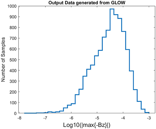
Figure 5. Distribution of log 10(|max{−Bz}|) values, where max{−Bz} is in G.
Regardless of the experiment:
1. The data were separated into 2 vectors, grouped by “storm” (; 82% of the data) and “no storm” (; 18% of the data).
2. The pointers to those two groups were randomly permuted, thus shuffling the data.
3. Two-thirds of the pointers were used for training, and one-third for testing, maintaining the 82 to 18% ratio of “storm” to “no storm” in both the training and testing data.
4. The input observations (be it magnetic field components of Stokes parameters) are in the solar equator plane in quadrature with Earth, along the ŷ direction. The field of views (FOVs) are identical in both experiments (x ∈ [1.0, 2.6]R⊙, z ∈ [−0.8, 0.8]R⊙). The observer is located at infinite distance from the origin, so that the lines-of-sight are parallel to each other for all image pixels.
5. The architecture of the FNN in each experiment remained the same regardless of the input data. However, for each different type of input the FNN was retrained, as the numerical values of the weights and bias is dependent on the type of input data (e.g., (L/I, Az), or V/I).
6. The FNN were run on an Intel CORE i7 9th generation CPU with 16 GB of RAM. The CNN were run on a NVIDIA Quadro P6000 GPU with 24 GB GDDR5X.
3.1. Experiment 1: Input Data
The G&L model is run to generate a total of 36288 magnetic 3D magnetic flux ropes that span a 5D parameter space (see Table 1). Two thirds (24192 flux ropes, 19847 “storm” + 4345 “no storm”) were used for training the machine learning algorithms and one third (12096 = 9923 “storm” + 2173 “no storm”) was used for testing the quality of the predictions. For Experiment 1, a single input sample showing a slice of all three magnetic field components Bx, By, and Bz, is given in the left panel of Figure 6, represented by a slice of the 3D datacube at the y = 0 plane. At present, no instrument can provide such input off the solar limb, but this Experiment is by design but a sanity-check test for the overall machine-learning pipeline.
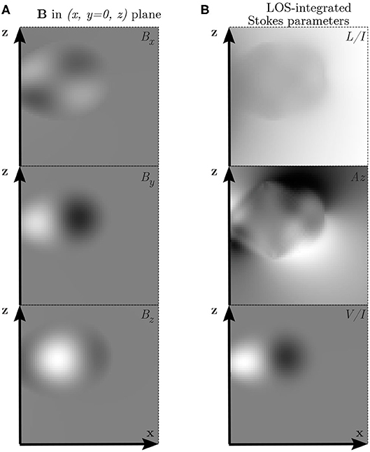
Figure 6. Left: an example of input for Experiment 1, three components of the magnetic field evaluated in the y = 0 plane, which is equivalent to an observation in quadrature to Earth. (This is akin to a vector magnetogram observed in the quadrature in the (x, y = 0, z) plane.) Right: an example of input for Experiment 2, three synthetic spectropolarimetric images, as they would appear to the same observer. These data are for f = 2.1R⊙, Ω = 35°, σ = 180°, τ1 = 3.38, θ = 7°. The field of view (FOV) is the same in all panels: x ∈ [1.0, 2.6]R⊙, z ∈ [−0.8, 0.8]R⊙.
Although Figure 6 shows gray-scale images, the input for Experiment 1 are 64 × 64 matrices of magnetic-field values in Gauss. While We are using the concept of image pattern recognition architectures (but with regression) to see if we can, instead of the byte-scaled images, use matrices that have values of a coronal magnetic field or its corresponding Stokes parameters that, for example, can range continuously from 0.7235 to 3.52513 × 10⁻⁵ to -0.764515. Further, for both FNNs we convert the input from a 64 × 64 matrix into a 4096 × 1 vector.
For the training of the FNN for Experiment 1 (hereafter FNN1), only one of these magnetic field components should be needed as an input (given as a 4069 × 24192 matrix); this is because, in this experiment, FNN1 is a binary classifier for a self-similar mapping—which means that due to the underlying symmetry of the solution, the number of variables is reduced. For training of the CNN for Experiment 1 (hereafter CNN1), we use all 3 channels as input (given as a 64 × 64 × 3 matrix), since although we still have a self-similar mapping, we are trying to estimate a number, max{−Bz}, to at least one decimal place of accuracy that varies over 5 orders of magnitude, not just (1, “storm”) or (0, “no storm”) as in FNN2. Note that CNN1 predicts the output that is simply a scaled-down version of the input, evaluated at a point. CNN1 is simply finding this scaling or mapping, which is what NNs are very good at.
3.2. Experiment 1: FNN and CNN Architecture
The first network, FNN1, is an FNN with one hidden layer. Its architecture is given in Figure 7 and its properties are listed below. The figure is generated by the simple command “view [(name of the NN)]” in MATLAB's Deep Learning Toolbox.
1. FNN1 has an input of a vector 4096 by 1, representing either the Bx, By, or Bz component of a GLOW flux rope.
2. It has 1 hidden layer with 10 neurons. In the Figure 7, the box with “w” and the box with “b” represent the weights and the biases for that layer, respectively.
3. The hyperbolic tangent curve in the hidden layer box indicates that we are using a tanh activation function. Approximating a binary classifier, where the probabilities fall between certain ranges, is easier with combinations of tanh(x) than the more popular piecewise linear functions (ReLu, e.g., Glorot et al., 2011) that is used in more complex NN.
4. The hidden layer is then connected to the output layer that uses a soft-max activation function, to calculate the probabilities of the ICME being a “storm” or “no storm,” represented by the graph with red dots.
5. Lastly, the cross-entropy loss function is used to measure the performance of the network against the true labels.
6. The stochastic gradient descent as the optimization algorithm.
7. The network was trained for 500 epochs.
8. MATLAB's feedforwardnet in the Deep Learning Toolbox was used.
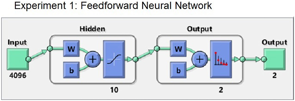
Figure 7. The feedforward fully connected network (FNN) used in Experiment 1 (FNN1). The letters “w” and “b” denote weights and biases, respectively; the full description of the scheme is given in the itemized list in section 3.2.
The final output is a probability p, 0 ≤ p ≤ 1. For this paper, we assume that if p ≥ 0.8 then the output is classified as a “storm”; if p ≤ 0.2 it is a “no storm”; if 0.2 < p < 0.8 we assume the network was unable to classify the output (in other words, the results are inconclusive).
All the “storms” correctly identified by the feedforward network are then passed into CNN1 for measuring the strength of log10{max{−Bz}} of the passing CME. The architecture of CNN1 for Experiment 1 is given in Figure 8 with its properties listed below. The figure is generated by the simple command “analyzeNetwork([name of the NN])” in MATLAB's Deep Learning Toolbox.
1. The first layer is an image input layer of 3 channels (that is, the values of Bx, By, Bz near the Sun). Consequently, it has dimension of 64 × 64 × 3.
2. There are two 2D convolutional layers, the first with 8 16 × 16 filters, the second with 20 8 × 8 filters. CNN1 is a shallow network due to the fact that we are simply mapping the magnetic field to a self-similar counterpart.
3. Each convolutional layer is followed by a ReLU activation function (Glorot et al., 2011).
4. Each ReLu layer is followed by a maxpooling layer, taking the maximum value from each 2 × 2 pixel region, resulting in a reduction of the matrix by a factor of 4.
5. The last layer is a fully connected layer which gives a prediction for log10{max{−Bz}}.
6. The error, compared to ground truth, is calculated by the root mean square error function and optimized through backpropagation with the Adam optimizer (Kingma and Ba, 2014).
7. The output values were normalized using a linear translation to between 0 and 1.
8. It was trained on 100 epochs.
9. A batch size of 567 was used.
10. The initial learn rate was set at 0.001.
11. The learning rate schedule was a piecewise drop with a learn rate drop of 0.75 and a learn rate drop period of 6.
12. An L2 Regularization of 10−4 was added.
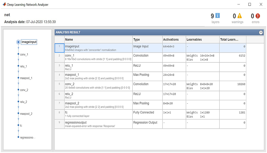
Figure 8. The 9 layer architecture of the convolutional neural network (CNN) constructed for Experiment 1 (CNN1) with the number of activations per layer and total number of learnable weights and bias in the convolutional layers and fully connected layer.
3.3. Experiment 2: Input Data
For Experiment 2, the input data are synthetic spectropolarimetric data corresponding to the magnetic fields generated for Experiment 1. A single input sample of the 36,288 synthetic Stokes observables is shown in the right panel of Figure 6. Although Figure 6 shows gray-scale images, the input for Experiment 2 are 64 × 64 matrices of the Stokes vector values in the same FOV and with the same resolution as Experiment 1. We use FORCOMP (CLE) package (Judge and Casini, 2001) of FORWARD suite (Gibson et al., 2016) in SolarSoft IDL (Freeland and Handy, 1998), to synthesize the components of the Stokes vector, (I, Q, U, V). In this work we use an alternative vector, which is derived from the Stokes vector: (I, L, Az, V). We further focus on the last three components of it, normalized by the intensity I, (L/I, Az, V/I). and contain the same information as Q and U. We find this representation more useful because it describes the linear polarization in terms of magnitude (L/I) and polarization angle (Az). In particular, it allows us to plot the polarization angle with respect to the local vertical (solar radial coordinate) and show how linear polarization is rotated in the presence of magnetic field. It also lets us immediately identify regions of highly reduced linear polarization associated with van Vleck angles and magnetic nulls (Gibson, 2018).
In this experiment, we are mapping observables measured in one space (Stokes data) to those measured in another space (magnetic field strength). The input and output data is no longer related by a mere scaling factor as in Experiment 1. Therefore, we will use either linearly polarized light (L/I, Az), or circularly polarized light (V/I), or the combination of the two, as various input data into the FNN constructed for Experiment 2 (hereafter FNN2) to understand the contribution of each to the results. Those that are classified correctly as “storms” are then inputted into the CNN architecture for Experiment 2 (hereafter CNN2).
3.4. Experiment 2: FNN and CNN Architecture
The fact that the functional mapping with the NNs is no longer self-similar and consequently, we do not have a reduction in the variables, will alter how we set up the architecture, requiring more degrees of freedom. In addition, we are passing the original G&L data through a highly non-linear model to synthesize Stokes images from the full-MHD variables, and yet we still expect CNN2 to map back to the original max{−Bz} output of the G&L model.
The architecture of FNN2 for Experiment 2 is given in Figure 9. All the properties are the same as for FNN1 from Experiment 1, except for those enumerated below.
1. FNN2 has an input of a vector 4096 × 1, 8192 × 1, or 12, 288 × 1, depending on whether we are inputting V/I, (L/I, AZ), or all three channels.
2. It has 1 hidden layer but now with 20 neurons.
3. There is a L2 regularization added with a parameter of 5e-4.
4. It was trained for 1,500 epochs.
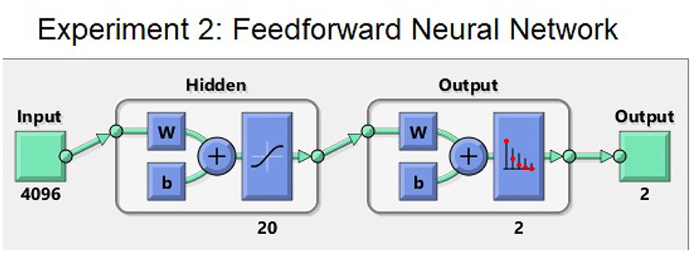
Figure 9. The feedforward fully connected network used in Experiment 2 (FNN2) The full description of the scheme is given in the itemized list in section 3.4.
As in Experiment 1, those events classified correctly as “storms” (i.e., the above mentioned p ≥ 0.8) are then inputted into CNN2. The architecture of CNN2 is given in Figure 10 and its properties are listed below.
1. In the case for the Stokes parameters, the input layer can either be of size 64 × 64 × 1, 64 × 64 × 2, or 64 × 64 × 3, depending on how many channels we are using.
2. There are now three 2D convolutional layers, the first with 10 16 × 16 filters, the second with 64 8 × 8 filters, and the third with 128 4 × 4 filters.
3. The initial random weights for each convolutional layer are defined using He initialization (He et al., 2015).
4. Each convolutional layer is followed by a ReLU activation function (Glorot et al., 2011).
5. Each ReLu layer is followed by a maxpooling layer, taking the maximum value from each 2 × 2 pixel region, resulting in a reduction of the matrix by a factor of 4.
6. The last layer is a fully connected layer which gives a prediction for log10{max{−Bz}}.
7. Again, the error was calculated by the root mean square error function and optimized with the Adam optimizer (Kingma and Ba, 2014).
8. Again, the output values for training were normalized using a linear translation to between 0 and 1.
9. V/I was multiplied by 103 so that it would be of the same order of magnitude as L/I and Az for training.
10. It was trained on 160 epochs.
11. A batch size of 735 was used.
12. The initial learn rate was set at 0.0015.
13. The learning rate schedule was a piecewise drop with a learn rate drop of 0.75 and a learn rate drop period of 10.
14. An L2 Regularization of 3 × 10⁻⁴ was added.
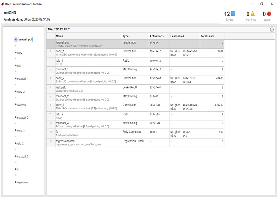
Figure 10. Twelve layer architecture of CNN2 with the number of activations per layer and total number of learnable weights and bias in the convolutional layers and fully connected layer.
4. Results
4.1. Experiment 1
This first experiment is a proof of concept. Essentially, using Bxyz near Sun as inputs and predicting Bz at 1AU means we are simply trying to teach NNs to predict a simple scaling of a number. If we can not succeed in this, then we cannot even hope to replace the G&L model output at the Earth with model output from MHD CME solar wind models, nor can we hope to predict the strength of magnetic field in passing ICMEs from coronal spectropolarimetric observations, as is done in Experiment 2 (albeit using synthetic observations).
We compare the results of the first (predictor, “storm” / “no storm”) NN against random guesses. Table 2 shows the outcome of random guessing: a guess was phrased (with probability of the outcomes weighted by their known ratio in the data), then an outcome was selected. The numbers in Table 2 can be easily calculated analytically as follows. Consider N events, out of which qN are storms, and (1 − q)N are not storms (0 ≤ q ≤ 1). Suppose the random guesser knows the value of q a priori, but makes predictions at random, weighted by q. It will classify qN events as storms. However, if predictions are truly random, amongst these qN events the fraction of actual storms will still be q; therefore, a random guesser will correctly predict a storm for q2N events, and will make false positive prediction for (1 − q)qN events; likewise, the amount of events correctly predicted as not storms and the amount of false negatives would be (1 − q)2N and q(1 − q)N respectively. In our case, q = 9923/12096 ≈ 0.82. A successful FNN prediction must result in a table more diagonal than Table 2.
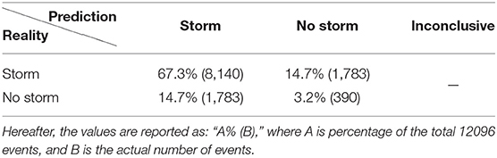
Table 2. No FNN, random guess (weighted by storm:no storm ratio).
Tables 3–5 show the results when only one of the components was taken as input. Using either of the three components, the predictor-based FNN1 can predict the outcome (“storm” / “no storm”) significantly better than a random guess. The Bz input produces the best predictions for the output, which is hardly surprising. The Bx input results in the worst prediction of the three (but still significantly better than a random guess). This could be caused by the fact that the ŷ and ẑ components of the flux rope are coupled by the orientation parameter σ, while the component is independent of both. However, even in the case of using Bx as input to the binary classifier, the ROC curve (a statistical tool to give the diagnostic ability of a binary classifier) gives excellent results with an AUC (area under curve) of 0.95 (a perfect predictor would have AUC=1, that is a zero false positive rate) as shown in Figure 11.

Table 3. Experiment 1: FNN1 using Bx only.
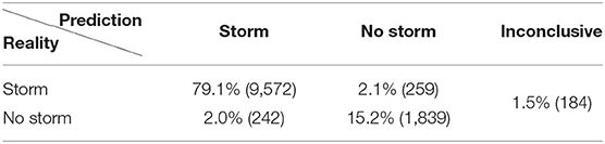
Table 4. Experiment 1: FNN1 using By only.
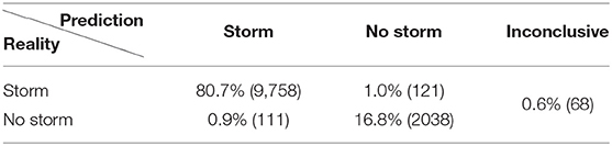
Table 5. Experiment 1: FNN1 using Bz only.
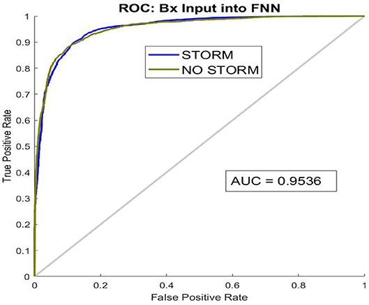
Figure 11. The ROC (Receiver Operator Characteristic) curve for the binary classifier FNN1 with Bx input. An AUC > 0.9 is considered excellent.
We further examine the efficiency of CNN1, the regression, for predicting the strength of the storm. We use the outcome of the FNN1 classifier based on Bx component as an input since, as is evident from the previous paragraph, it proves the most challenging scenario for the first NN, and, consequently, the results based on By and Bz are expected to supersede it. The results, shown in Figure 12, demonstrate that the predictions are successful, which ultimately means that the NN pipeline is overall working well.
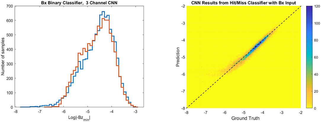
Figure 12. A histogram (blue is ground truth) and scatter plot, of ground truth vs. predictions of CNN1, when using the Bx component of magnetic field at the Sun as input for the binary classifier FNN1 and then feeding the events labeled as “storms” into the 9 layer CNN1 to predict the value of max{−Bz}. The color bar indicates the number of samples. The axes in the scatter plot are that of log10{max{−Bz}}, and in both plots the units of max{−Bz} are G.
4.2. Experiment 2
The first part of the experiment is to understand how well the binary classifier performs if the input is (a) only linearly polarized light, (b) only circularly polarized light, and (c) using both, comparing to random choice shown in Table 2. Recall that the output of the classifier is a number p (where 0 ≤ p ≤ 1) indicating a probability, and we interpret p ≥ 0.8 as a storm, p ≤ 0.2 as no storm, and 0.2 < p < 0.8 as inconclusive, the results are given in Tables 6–8. First, notice that the input of just (L/I, Az) gives results that are worse than if the guess was random. Also note that approximately 30% of the results (3570 of 12096) are inconclusive. Secondly, when using only V/I as an input, the true positives could be determined to within 93.5%, the true negatives to within 73%, and only 7% of the cases are inconclusive. By using all 3 Stokes components, we get a slight improvement of ≤ 1% which could easily be considered within the noise of the classifier. However, what is impressive is that if the ROC is plotted for the case where we use all the 3 Stokes components, as seen is in Figure 13, the AUC is 0.99.
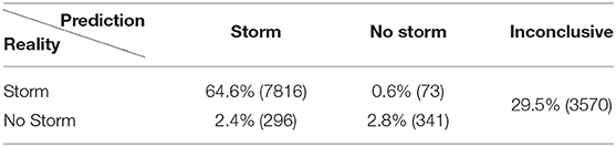
Table 6. FNN2 using L/I and Az only.
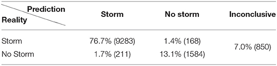
Table 7. FNN2 using V/I only.

Table 8. FNN2 using L/I, Az, and V/I.
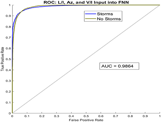
Figure 13. The ROC (Receiver Operator Characteristic) curve for the binary classifier FNN2 with all 3 Stokes components as input (L/I, Az, V/I). An AUC > 0.9 is considered excellent.
The second part of this experiment takes those samples that correctly classified as storms and run them through the 3 channel CNN2 to predict the strength of the storm. Figure 14 shows the results both in histogram form and as scatter plots of ground truth vs. prediction. First, note that just considering the V/I inputs from the binary classification results in a histogram that seems to overall fit the true data (blue) rather well (except for maybe accruing larger sample sizes for peak values around 10−4.25G). However, the scatter plot shows that the slope is not quite unity and there is a slight bias to overpredict values of . In this case, the Pearson correlation coefficient is 0.95. If instead we use CNN2 trained on the data from the binary classifier that includes all 3 channels (L/I, Az, V/I), we see that the bias is corrected and the predictions line up perfectly with the ground truth. The Pearson correlation coefficient in this case is 0.98.
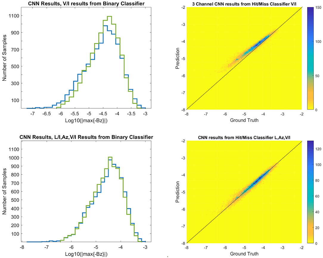
Figure 14. Two representations, histogram and scatter plot, of predictions of CNN2 vs. ground truth, on the subset of events which FNN2 has predicted was a “storm.” Top: when using only circularly polarized light, V/I, as input to FNN2. Bottom: when using both linearly and circularly polarized light, (L/I, Az, V/I), as input to FNN2. The color bar indicates the number of samples. Blue lines are ground truth in both histograms. The axes in the scatter plot are that of log10{max{−Bz}}, and in all panels the units of max{−Bz} are G.
Finally, we calculate the relative root square error for the accuracy of predictions for both NNs. We use the following definition:
where for brevity we denoted Ξ = max{−Bz}, GT stands for “ground truth,” and “NN” stands for “NN-predicted value.” We find that, given three components of B near Sun, CNN1 can predict max{−Bz} at 1AU at 97% accuracy (E = 0.97), and for three components of the Stokes vector near Sun as input, CNN2 can predict max{−Bz} at 1AU with 95% accuracy (E = 0.95).
5. Conclusions
In this paper we have developed a machine learning algorithm to set a baseline for testing the efficacy of coronal spectropolarimetric measurements for predicting max{−Bz} at the Earth. We have found that the circularly polarized light maintains the crucial magnetic field information for making a good prediction, at least for the simple model we examined. This is not unexpected, as circular polarization is directly related to the line-of-sight (in our case, By) field strength (see Rachmeler et al., 2012, for further discussion). However, the polarization signal is a result of the line-of-sight integration of the data, and disambiguation is required to derive the 3D structure of the field. The ability of neural networks to perform this disambiguation, which only yields information about By signal, and then to form meaningful Bz predictions at a later time, demonstrates that machine learning is a valuable asset for space weather predictions. Linearly polarized light on its own does not do so well, as it is not sensitive to the magnetic field strength but only to its geometry. It nonetheless proves to be important when considered in combination with circularly polarized light. Indeed, the most accurate prediction arises when all the components of the Stokes vector are included.
Full-MHD simulations of interplanetary CME evolution from Sun to Earth are typically computationally expensive. CNN allows us to explore a large space of CME models with different characteristics to study which initial states result in the strongest geomagnetic storm. The role of CNN in this case is, given either magnetic field or the synthetic spectropolarimetric observables of a CME near Sun in quadrature view, paired with max{−Bz} values at Earth, to predict magnetic field inside a CME at later time and therefore to facilitate the magnetic storm predictions.
This project could be considered as preparatory work for future projects. Some of these could include, for example, exploring near-Sun signatures of CMEs in other channels (such as extreme ultraviolet), and in the addition to predicting max{−Bz}, to also predict other parameters of the storm (such as its duration).
In the introduction, we mention two major factors influencing our ability to use near-Sun spectropolarimetric signatures of CMEs for space weather predictions. Our work explicitly addresses the first factor, i.e., the capability of the neural networks to use near-Sun spectropolarimetric signatures for predicting magnetic field strength in the erupting flux rope. The evolution of the CME from Sun to Earth, i.e., the second factor mentioned in the introduction, requires a model that can take into account the changes of the structure as it interacts with the solar wind. Provornikova et al. (2020, in preparation) will show an example of such a simulation, as part of a project which is currently in development (NASA award 80NSSC17K0685). The project will yield a database of tens of thousands of MHD simulations, in which various configurations of a G&L flux rope will be used as inputs, along with realistic solar wind models (Arge et al., 2004), and their interaction will be modeled in MHD simulations (Merkin et al., 2016). We tailored our input and output for maximal compatibility with this project. Our plan is to follow up the current work with an equivalent analysis using a large number of MHD runs of CME propagation through the solar wind. By doing this, we will be able to determine how much information is retained even when non-ideal evolution of ICME in the solar wind between Sun and Earth is taken into consideration.
Data Availability Statement
The raw data supporting the conclusions of this article will be made available by the authors upon request, without undue reservation.
Author Contributions
AM have designed and produced the database of GLOW flux rope models used in the project, including magnetic, spectropolarimetric, and near-Earth data. She assisted in their interpretation and analysis. NF created and trained CNNs and FNNs, as well as analyzed their performance in predictions. SG was the author of the model and the codes used in the project, she provided consultations on GLOW model and assisted with producing and interpreting synthetic spectropolarimetric data. AM, NF, and SG participated in writing the manuscript.
Funding
This work was supported by the NASA award 80NSSC17K0685 and the National Center for Atmospheric Research, which is a major facility sponsored by the National Science Foundation under Cooperative Agreement No. 1852977.
Conflict of Interest
The authors declare that the research was conducted in the absence of any commercial or financial relationships that could be construed as a potential conflict of interest.
Acknowledgments
SG and AM acknowledge further support from NASA grant number 80NSSC17K0685. We thank Ricky Egeland, who was the NCAR internal referee, as well as the two external referees, for providing many valuable comments which have improved the paper.
Footnotes
1. ^(A specific analytical solution for a toroidal flux rope embedded in a spherical shell, which is a common object of study, e.g., in laboratory plasma research and in solar physics, e.g., Hagenson and Krakowski, 1987; Gibson and Low, 1998; Borovikov et al., 2017, etc.)
2. ^We hereafter assume a system of units in which R⊙ = 1.
3. ^To see this, one could express both τ1 and the coordinates of the special points via x0, r0, and a: ; xA = x0 − r0 − a, etc.
4. ^In Gibson and Low (1998), the stretching parameter a is introduced in MHD equations as the additional gravity term. Therefore, a < 0 will physically mean a gravity force directed away from the Sun's center.
5. ^In the sense of
References
Arge, C. N., Luhmann, J. G., Odstrcil, D., Schrijver, C. J., and Li, Y. (2004). Stream structure and coronal sources of the solar wind during the May 12th, 1997 CME. J. Atmos. Solar Terres. Phys. 66, 1295–1309. doi: 10.1016/j.jastp.2004.03.018
Baker, D. N. (2013). “The major solar eruptive event in July 2012: defining extreme space weather scenarios (invited),” in AGU Fall Meeting Abstracts, Vol.2013, SM13C–04.
Bak-Steslicka, U., Gibson, S. E., Fan, Y., Bethge, C., Forland, B., and Rachmeler, L. A. (2013). The magnetic structure of solar prominence cavities: new observational signature Revealed by Coronal Magnetometry. Astrophys. J. Lett. 770:L28. doi: 10.1088/2041-8205/770/2/L28
Borovikov, D., Sokolov, I. V., Manchester, W. B., Jin, M., and Gombosi, T. I. (2017). Eruptive event generator based on the Gibson-Low magnetic configuration. J. Geophys. Res. 122, 7979–7984. doi: 10.1002/2017JA024304
Chen, P. F. (2011). Coronal mass ejections: models and their observational basis. Liv. Rev. Solar Phys. 8:1. doi: 10.12942/lrsp-2011-1
Cliver, E. W., and Dietrich, W. F. (2013). The 1859 space weather event revisited: limits of extreme activity. J. Space Weather Space Clim. 3:A31. doi: 10.1051/swsc/2013053
Dove, J. B., Gibson, S. E., Rachmeler, L. A., Tomczyk, S., and Judge, P. (2011). A Ring of Polarized Light: Evidence for Twisted Coronal Magnetism in Cavities. Astrophys. J. Lett. 731:L1. doi: 10.1088/2041-8205/731/1/L1
Eastwood, J. P., Biffis, E., Hapgood, M. A., Green, L., Bisi, M. M., Bentley, R. D., et al. (2017). The economic impact of space weather: where do we stand? Risk Anal. 37, 206–218. doi: 10.1111/risa.12765
Fan, Y., and Gibson, S. E. (2003). The emergence of a twisted magnetic flux tube into a preexisting coronal arcade. Astrophys. J. Lett. 589, L105–L108. doi: 10.1086/375834
Fan, Y., and Liu, T. (2019). MHD simulation of prominence-cavity system. Front. Astron. Space Sci. 6:27. doi: 10.3389/fspas.2019.00027
Forland, B. C., Gibson, S. E., Dove, J. B., Rachmeler, L. A., and Fan, Y. (2013). Coronal cavity survey: morphological clues to eruptive magnetic topologies. Solar Phys. 288, 603–615. doi: 10.1007/s11207-013-0361-1
Freeland, S. L., and Handy, B. N. (1998). Data analysis with the solarSoft system. Solar Phys. 182, 497–500. doi: 10.1023/A:1005038224881
Gibson, S. (2015). Coronal cavities: observations and implications for the magnetic environment of prominences. Astrophys. Space Sci. Libr. 415:323. doi: 10.1007/978-3-319-10416-4-13
Gibson, S., Kucera, T., White, S., Dove, J., Fan, Y., Forland, B., et al. (2016b). FORWARD: a toolset for multiwavelength coronal magnetometry. Front. Astron. Space Sci. 3:8. doi: 10.3389/fspas.2016.00008
Gibson, S. E. (2018). Solar prominences: theory and models. Fleshing out the magnetic skeleton. Liv. Rev. Solar Phys. 15:7. doi: 10.1007/s41116-018-0016-2
Gibson, S. E., and Low, B. C. (1998). A time-dependent three-dimensional magnetohydrodynamic model of the coronal mass ejection. Astrophys. J. 493, 460–473. doi: 10.1086/305107
Glorot, X., Bordes, A., and Bengio, Y. (2011). “Deep sparse rectifier neural networks,” in Proceedings of Machine Learning Research, (Fort Lauderdale, FL: JMLR Workshop and Conference Proceedings), 315–323. Available online at: http://proceedings.mlr.press/v15/glorot11a.html
Goodfellow, I., Bengio, Y., and Courville, A. (2016). Deep Learning. Cambridge, MA: MIT Press. Available online at: http://www.deeplearningbook.org
Hagenson, R. L., and Krakowski, R. (1987). The Spheromak as a Compact Fusion Reactor. Tech. rep., Los Alamos National Lab., NM (USA).
He, K., Zhang, X., Ren, S., and Sun, J. (2015). “Delving deep into rectifiers: Surpassing human-level performance on imagenet classification,” in Proceedings of the 2015 IEEE International Conference on Computer Vision (ICCV), ICCV '15, p. 1026–1034, USA, IEEE Computer Society. doi: 10.1109/ICCV.2015.123
Judge, P. G., and Casini, R. (2001). A Synthesis Code for Forbidden Coronal Lines, volume 236 of Astronomical Society of the Pacific Conference Series, p. 503.
Kilpua, E. K. J., Lugaz, N., Mays, M. L., and Temmer, M. (2019). Forecasting the Structure and Orientation of Earthbound Coronal Mass Ejections. Space Weather, 17:498–526. doi: 10.1029/2018SW001944
Kingma, D., and Ba, J. (2014). Adam: A Method for Stochastic Optimization. arXiv e-prints, art. arXiv:1412.6980.
Knipp, D. J., and Gannon, J. L. (2019). The 2019 National Space Weather Strategy and Action Plan and Beyond. Washington, DC: The National Academies Press. doi: 10.1029/2019SW002254. Available online at: https://www.whitehouse.gov/wp-content/uploads/2019/03/National-Space-Weather-Strategy-and-Action-Plan-2019.pdf
Manchester, W., Kilpua, E. K. J., Liu, Y. D., Lugaz, N., Riley, P., Torok, T., et al. (2017). The Physical Processes of CME/ICME Evolution. Space Sci. Rev. 212:1159–1219. doi: 10.1007/s11214-017-0394-0
Merkin, V. G., Lyon, J. G., Lario, D., Arge, C. N., and Henney, C. J. (2016). Time-dependent magnetohydrodynamic simulations of the inner heliosphere. J. Geophys. Res. 121:2866–2890. doi: 10.1002/2015JA022200
National Research Council. (2008). Severe Space Weather Events: Understanding Societal and Economic Impacts: A Workshop Report. Washington, DC: The National Academies Press. doi: 10.17226/12507
Rachmeler, L. A., Casini, R., and Gibson, S. E. (2012). Interpreting Coronal Polarization Observations. In T. R. Rimmele, A. Tritschler, F. Wöger, M. Collados Vera, H. Socas-Navarro, R. Schlichenmaier, M. Carlsson, T. Berger, A. Cadavid, P. R. Gilbert, P. R. Goode, and M. Knölker, editors, Second ATST-EAST Meeting: Magnetic Fields from the Photosphere to the Corona., volume 463 of Astronomical Society of the Pacific Conference Series, 227, Orem, UT, December 2012.
Ruiz Cobo, B., and del Toro Iniesta, J. C. (1992). Inversion of Stokes Profiles. Astrophys. J. 398:375. doi: 10.1086/171862
Schou, J., Scherrer, P. H., Bush, R. I., Wachter, R., Couvidat, S., Rabello-Soares, M. C., et al. (2012). Design and Ground Calibration of the Helioseismic and Magnetic Imager (HMI) Instrument on the Solar Dynamics Observatory (SDO). Solar Phys. 275:229–259. doi: 10.1007/s11207-011-9842-2
Svozil, D., Kvasnicka, V., and Pospichal, J. (1997). Introduction to multi-layer feed-forward neural networks. Chemometrics and Intelligent Laboratory Systems 39:43–62. doi: 10.1016/S0169-7439(97)00061-0
The MathWorks (2019). Deep Learning Toolbox. Available online at: https://www.mathworks.com/help/deeplearning/
Webb, D. F., and Howard, T. A. (2012). Coronal Mass Ejections: Observations. Living Rev. Solar Phys. 9:3. doi: 10.12942/lrsp-2012-3
Keywords: coronal mass ejection, initiation and propagation, convolutional neural network (CNN), Gibson and Low model, interplanetary CMEs, spectropolarimetric data classification
Citation: Malanushenko A, Flyer N and Gibson S (2020) Convolutional Neural Networks for Predicting the Strength of the Near-Earth Magnetic Field Caused by Interplanetary Coronal Mass Ejections. Front. Astron. Space Sci. 7:62. doi: 10.3389/fspas.2020.00062
Received: 15 April 2020; Accepted: 05 August 2020;
Published: 18 September 2020.
Edited by:
Bala Poduval, University of New Hampshire, United StatesReviewed by:
Emilia Kilpua, University of Helsinki, FinlandTeresa Nieves-Chinchilla, National Aeronautics and Space Administration, United States
Copyright © 2020 Malanushenko, Flyer and Gibson. This is an open-access article distributed under the terms of the Creative Commons Attribution License (CC BY). The use, distribution or reproduction in other forums is permitted, provided the original author(s) and the copyright owner(s) are credited and that the original publication in this journal is cited, in accordance with accepted academic practice. No use, distribution or reproduction is permitted which does not comply with these terms.
*Correspondence: Anna Malanushenko, YW5ueUB1Y2FyLmVkdQ==