Probing the Thermodynamic State of a Coronal Mass Ejection (CME) Up to 1 AU

Mishra, Wageesh; Wang, Yuming; Teriaca, Luca; Zhang, Jie; Chi, Yutian

doi:10.3389/fspas.2020.00001

ORIGINAL RESEARCH article

Front. Astron. Space Sci., 30 January 2020

Sec. Stellar and Solar Physics

Volume 7 - 2020 | https://doi.org/10.3389/fspas.2020.00001

This article is part of the Research Topic Magnetic Flux Ropes: From the Sun to the Earth and Beyond View all 11 articles

Probing the Thermodynamic State of a Coronal Mass Ejection (CME) Up to 1 AU

$\nWageesh Mishra$ Wageesh Mishra¹^*

Yuming Wang²

Luca Teriaca¹

Jie Zhang³

Yutian Chi²

¹Max Planck Institute for Solar System Research, Göttingen, Germany
²CAS Key Laboratory of Geospace Environment, Department of Geophysics and Planetary Sciences, University of Science and Technology of China, Hefei, China
³Department of Physics and Astronomy, George Mason University, Fairfax, VA, United States

Several earlier studies have attempted to estimate some of the thermodynamic properties of Coronal Mass Ejections (CMEs) either very close to the Sun or at 1 AU. In the present study, we attempt to extrapolate the internal thermodynamic properties of 2010 April 3 flux rope CME from near the Sun to 1 AU. For this purpose, we use the flux rope internal state (FRIS) model which is constrained by the kinematics of the CME. The kinematics of the CME is estimated using the STEREO/COR and HI observations in combination with drag based model (DBM) of CME propagation. Using the FRIS model, we focus on estimating the polytropic index of the CME plasma, heating/cooling rate, entropy changing rate, Lorentz force and thermal pressure force acting inside the CME. Our study finds that the polytropic index of the selected CME ranges between 1.7 and 1.9. This implies that the CME is in the heat-releasing state (i.e., entropy loss) throughout its journey from the Sun to Earth. The hindering role of Lorentz force and contributing role of thermal pressure force in governing the expansion of the CME is also identified. On comparing the estimated properties of the CME flux rope from the FRIS model with the in situ observations of the CME taken at 1 AU, we find relevant discrepancies between the results predicted by the model and the observations. We outline the approximations made in our study of probing the internal state of the CME during its heliospheric evolution and discuss the possible causes of the observed discrepancies.

1. Introduction

Coronal mass ejections (CMEs) are the large-scale transients arising from the Sun and, being energetic plasma phenomena, they are the main driver of disturbances in the terrestrial space environment (Tousey, 1973; Hundhausen et al., 1984; Schwenn, 2006; Zhang et al., 2007; Baker, 2009; Chen, 2011; Webb and Howard, 2012). CMEs moving outside the field of view of coronagraphs are often referred to as interplanetary coronal mass ejections (ICMEs). Based on the in situ observations of ICMEs, a subset of them are named Magnetic clouds (MCs) as they show large and coherent rotation of the magnetic field vector, larger magnetic field, and a low plasma beta (Burlaga et al., 1981; Marubashi and Lepping, 2007; Wang et al., 2018). Such MCs are understood as flux ropes expanding during their heliospheric evolution while keeping their magnetic connection to the Sun (Larson et al., 1997; Gulisano et al., 2010). Solar-terrestrial physics studies have improved our understanding of different forces acting on the different parts of a CME, their kinematic evolution and space weather effects by using remote sensing and in situ spacecraft observations for several decades. However, the physical processes behind the formation of CMEs/ICMEs associated flux ropes, their acceleration and heating have not yet been understood completely (Forsyth et al., 2006; Chen, 2011; Webb and Howard, 2012; Harrison et al., 2018).

The heating and acceleration of the solar wind have been investigated extensively since the seminal work of Parker (1960). However, a majority of studies on CMEs that make use of white light imaging observations which only provide information on the plasma density, have not focused on understanding the thermodynamics of the CMEs. Near the Sun, some information on the thermodynamic state of a CME is obtained using the EUV spectral observations from the Ultraviolet Coronagraph Spectrometers (UVCS), Coronal Diagnostic Spectrometer (CDS), and Solar Ultraviolet Measurements of Emitted Radiation (SUMER) instruments aboard the SOlar and Heliospheric Observatory (SOHO) spacecraft (Akmal et al., 2001; Raymond, 2002; Ciaravella et al., 2003; Kohl et al., 2006; Bemporad and Mancuso, 2010). These studies suggested that there is a deposition of thermal energy into CMEs in the inner corona where they have a higher temperature than the ambient solar wind. To understand the dominant physical mechanism responsible for heating/cooling of expanding plasmoids in the heliosphere, it is necessary to probe the CME thermodynamic state at different distances from the Sun. The thermodynamic evolution of CMEs is often understood by using a polytropic approximation. The different value of the polytropic index for the CME plasma implies different rates of heating, which leads to a different evolution of the CME. An empirical determination of the polytropic index using in situ observations is possible if a CME can be observed by several radially-aligned spacecraft (Phillips et al., 1995). The global MHD modeling of ICMEs based on a polytropic approximation to the energy equation has been published by Riley et al. (2003) and Manchester et al. (2004). The combined information of density, temperature and ionization state of CMEs can be used to understand the physical processes within CME plasma.

Over the years, in situ measurements of ICMEs have been made using several spacecraft located over a range of heliocentric distances from the Sun. The studies on the thermodynamic treatment of ICMEs between 0.3 and 30 AU have been carried out using in situ observations of Voyagers, Ulysses, Helios, WIND, ACE, and STEREO spacecraft (Osherovich et al., 1993; Phillips et al., 1995; Wang and Richardson, 2004; Liu et al., 2006a). The studies have confirmed that CMEs have a lower temperature than that in the ambient solar wind (Burlaga et al., 1981; Richardson and Cane, 1993), and they have highly elevated ionic charge states (Lepri et al., 2001; Zurbuchen et al., 2003). The elevated charge states which freeze in relatively close to the Sun during the CME expansion are indicative of strong heating at CME source relative to the ambient solar wind. The occasional presence of singly charged helium and relatively low ionic charge states in ICMEs is found to be associated with low-temperature filament material on the Sun (Burlaga et al., 1998; Gruesbeck et al., 2012). Since the two spacecraft rarely get well co-aligned radially for recurrent observations of the plasma properties of the same CME at different distances (Skoug et al., 2000). Therefore, in general, in situ measurements do not allow us to examine the evolution of an individual CME as it travels away from the Sun. However, using a large amount of in situ observations of CMEs over different distances, one can adopt a statistical method to understand their thermodynamic evolution. Such a statistical approach assumes that an average of observed plasma parameters over many CMEs represents the properties of a typical CME. Using such approach, it has been statistically shown that both the density and magnetic field decrease faster in ICMEs than in the solar wind, but the temperature decreases slower in ICMEs than in the solar wind, and the expansion of an ICME is more like an isothermal process than an adiabatic one (Wang and Richardson, 2004; Liu et al., 2005, 2006a; Wang et al., 2005). Recently, using in situ observations of ICMEs at different distances between 0.3 and 1 AU, it was shown that there is a good correlation between the ejecta and sheath speeds, but low correlation between the magnetic field magnitudes in the sheath and ejecta (Janvier et al., 2019).

Although a few earlier studies have investigated the thermodynamic state of CMEs using remote sensing observations close to the Sun and in situ observations very far from the Sun. Thus, these studies provide CME thermal parameters only at a certain heliocentric distance and/or at a certain time. The pioneering attempt to investigate the internal state of an individual CME during its propagation in the outer corona (i.e., 2–70 R_⊙) was done by Wang et al. (2009) by developing a Flux Rope Internal State (FRIS) model. The model was further improved by Mishra and Wang (2018) and they applied it to the coronagraphic observations of a slow CME to understand the internal forces and thermodynamic properties (polytropic index, heating rate, entropy change, etc.). The use of coronagraphic observations in combination with the FRIS model allowed to track the thermodynamic evolution of a specific CME with distance from the Sun. This approach differs from earlier studies which provided a statistical result, over a large amount of data, on the variation of a few thermodynamic parameters with distance. The FRIS model is extremely advantageous as it probes the evolution of the CMEs thermodynamic state in terms of CMEs kinematics which can be accurately derived from available imaging observations. It is expected that CMEs with different kinematic characteristics may show different thermodynamic evolution in the heliosphere. Therefore, it would be an obvious next step to apply the FRIS model to different CMEs and understand their thermodynamic evolution.

In the present study, we attempt to apply the FRIS model to a fast CME of 3 April 2010. The CME did not decelerate much during it interplanetary propagation and could be identified as the fastest ICME to arrive near the Earth since the 2006 December 13 event (Liu et al., 2008, 2011). The 3 April 2010 CME had also caused a prolonged geomagnetic storm leading to a breakdown of a Galaxy 15 satellite for about 6 months. This CME has been extensively studied for its solar and interplanetary signatures, however its thermodynamic properties were so far not explored. Importantly, we estimate the thermodynamic properties of the selected CME up to 1 AU and compare the model extrapolated results with the in situ observations of the CME near the Earth. For the completeness, we briefly introduce the improved FRIS model and the parameters which can be derived using the model in section 2. The application of the model to the coronagraphic observations of the selected CME is made in section 3. The extrapolation of the CME kinematics and estimated thermodynamic properties is described in section 4. The results obtained from the observations with the aid of the FRIS model and their discussion are summarized in section 5.

2. Flux Rope Internal State (FRIS) Model for CME

The flux rope internal state (FRIS) model was first developed by Wang et al. (2009) and later by Mishra and Wang (2018). To better define the basis of the present study, we briefly describe the FRIS model here. The FRIS model treats the CME as an axisymmetric cylinder in the local scale with self-similar expansion during its heliospheric propagation (Figure 1). The model considers three global motions for a CME's flux rope characterized by linear propagation speed (υ_c), expansion speed (υ_e), and poloidal speed (υ_p) which are represented in the figure with black, red, and blue arrows respectively. Thus, under self-similar expansion and considering that magnetic field lines are frozen-in with the plasma flows, the density in the flux rope CME would have a fixed distribution. Further, the mass and angular momentum of the CME are assumed to be conserved. Thus, the average density in the flux rope would change with time as CME propagates away from the Sun. Under the assumption that the axial length of a CME flux rope is proportional to the distance (L) between the axis of the flux rope and the solar surface, the average density can be expressed in terms of L and radius (R) of the cross-section of the flux rope.

FIGURE 1

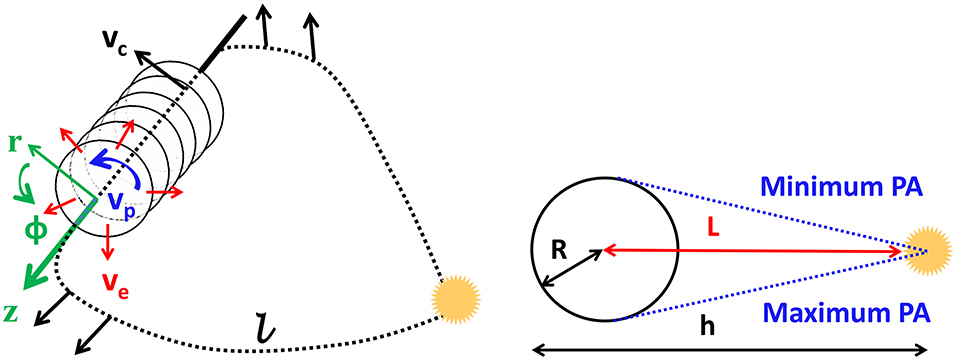
Figure 1. Left: A representative picture of a CME flux rope. The black dashed line indicates the looped axis of the flux rope with the axial length as l. A cylindrical coordinate system (i.e., r, ϕ, z) is attached to the axis of the flux rope (in green). Right: A representative picture for the cross-section of the CME flux rope. The radius of the flux rope is R, the distance from the flux rope axis to the solar surface is L, the distance of the CME leading edge from the Sun's center is h, and the minimum and the maximum position angles (PA) are shown with dotted blue lines (adapted from Mishra and Wang, 2018).

Further, using the laws of thermodynamics for a polytropic process, one can express the evolution of a thermodynamic variable, such as a change in entropy, in terms of average density and polytropic index (Γ). The FRIS model investigates the expanding propagation of a flux rope CME under thermal pressure force, Lorentz force from the axis to the boundary of the flux-rope, and centrifugal force due to the poloidal motion of the plasma. Therefore, one can derive the expressions for various forces by measuring the kinematics (i.e., L, R, and their derivatives) of a CME flux rope. The derivation of dynamic and thermodynamic variables is possible by involving several unknown constants dependent on the plasma and magnetic field parameters (e.g., distributions of density, poloidal speed, and magnetic vector potential, length of the flux rope, equivalent heat source and coefficient of conductivity, etc.) inside the flux rope CME. Therefore, in the model, the evolution of several thermodynamic parameters of the CME is expressed in terms of a time-dependent variable (λ) that can further be expressed in terms of the observed kinematic parameters of the CME and on several unknown coefficients introduced in the model. These introduced unknown coefficients (c₁₋₅) could be derived from the observed kinematics of the CMEs. The expressions for the coefficients depend on other unknown constants and their interpretation is given in the middle and bottom panels of Table 1. It is also evident that once the values of λ, its derivative, the coefficients, and CME kinematics are estimated, the expressions in the top panel of the table can be used to estimate several thermodynamic parameters of the CME.

\begin{array}{l} {(L R^{2})}^{γ - 1} = L^{γ - 1} R^{γ - 1} {[c}_{5} a_{e} + {(γ - 1) c_{4} a_{e} v_{c} - c_{3} c_{5} L^{- 1} \\ + c_{4} \frac{d a_{e}}{d t} L} R^{- 1} \\ + {(2 - γ) c_{3} c_{4} v_{c} L^{- 1} + (γ - 1) c_{4} a_{e} v_{e} L} R^{- 2} \\ + {(2 - γ) c_{3} c_{4} v_{e} - c_{2} c_{5} L - c_{1} c_{5} {} R}^{- 3} \\ + {(1 - γ) c_{1} c_{4} v_{c} - γ c_{2} c_{4} v_{c} L} R^{- 4} \\ \begin{matrix} + {(4 - γ) c_{1} c_{4} v_{e} L + (4 - γ) c_{2} c_{4} v_{e} L^{2} {} R}^{- 5}] \end{matrix} & (1) \end{array}

The relation between the unknown coefficients and the measurements of a CME flux rope is expressed in Equation (1). In the equation, L, R, υ_c, υ_e, a_e, and $\frac{d a_{e}}{d t}$ are the measurements of distance between the axis of the flux rope and the solar surface, the radius of the flux rope, propagation speed, expansion speed, expansion acceleration, and rate of change of expansion acceleration of the flux rope, respectively. γ is the heat capacity ratio (i.e., adiabatic index) which is 5/3 for monoatomic ideal gases. From the equation, it is clear that if we have the measurements L, R, and their time derivatives, the value of all the unknown coefficients c₁₋₅ can be estimated by fitting the Equation (1) to the measurements of the CME flux rope. Once the values of c₁₋₅ and λ is obtained from the model, several thermodynamic parameters of the CME can be estimated as evident from Table 1. From the table, we also note the presence of unknown factors which scale the estimated thermodynamic parameters. These factors forbid us to estimate the absolute value of most of the thermodynamic parameters of the CME, but allow to show their trend with time or heliocentric distance.

TABLE 1

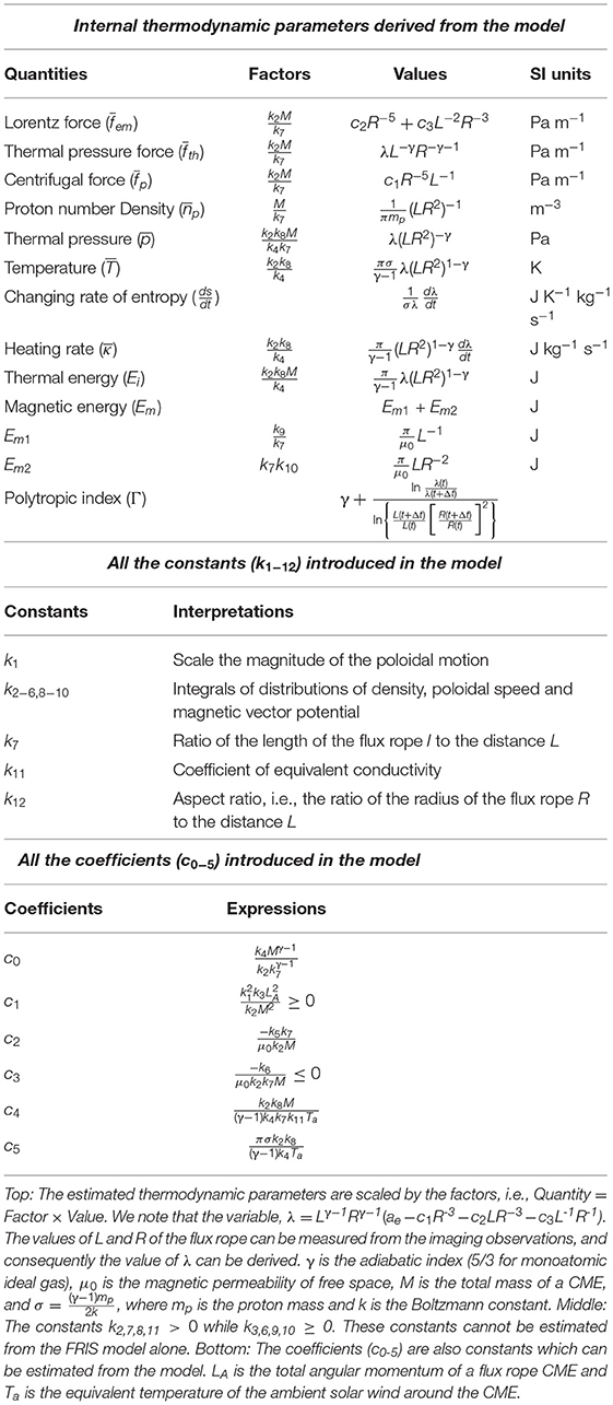
Table 1. List of the derived internal thermodynamic parameters, constants, and coefficients from FRIS model.

Using the FRIS model, we can infer the evolution of thermodynamic properties and internal forces of CMEs using the estimated kinematics of the CMEs as inputs in the model. Using multiple viewpoints observations, such as white light coronagraphic and heliospheric imaging observations from the twin STEREO spacecraft, and 3D reconstruction methods, it is possible to accurately estimate the CMEs deprojected kinematics as they propagate farther out from the Sun (Inhester, 2006; Thernisien et al., 2009; Mierla et al., 2010; Davies et al., 2013; Mishra et al., 2014; Harrison et al., 2018). If a CME could not be tracked continuously in imaging observations at larger distances from the Sun, one can implement the drag-based model (DBM) (Vršnak et al., 2013) and/or MHD models (Pomoell and Poedts, 2018) to derive the speed of the CME at those distances.

3. Application of the FRIS Model to the CME of 3 April 2010

The CME of 3 April 2010 was associated with the disappearance of a filament, coronal dimming, and a B7.4 long-duration flare from NOAA Active Region (AR) 1059 (Liu et al., 2011). The CME was observed as a halo by SOHO/LASCO-C2, in the SE quadrant by STEREO/COR1-A and in the SW quadrant by STEREO/COR1-B coronagraphs. To implement the FRIS model, as described in section 2, we require the radius of cross-section of the flux rope CME (R), the distance of the axis of the flux rope from the solar surface (L) and their derivatives.

3.1. Observations and Measurements From Imaging Observations

To derive the 3D kinematics (L, R, directions, etc.) of the selected CME, we used the Graduated Cylindrical Shell (GCS) model (Thernisien et al., 2006, 2009). The details about derivable parameters from GCS forward fitting model and procedures for its correct application have been discussed thoroughly in the literature (Lynch et al., 2010; Thernisien, 2011; Vourlidas et al., 2013; Wang et al., 2014; Mishra et al., 2015). The GCS model is applied first to the COR2 observations of the CME. We manually adjusted all the six free parameters of the GCS model to closely match the modeled flux rope geometry with the observed CME flux rope. The GCS fitted wireframe contour obtained after the application of the GCS model to the contemporaneous coronagraphic images of the CME from the three viewpoints are shown in Figure 2. However, it is difficult to apply the GCS model to HI images due to the faint structure of CMEs at large distances from the Sun. Despite the ambiguous tracking of the CME flux rope in HI1 field of view, we applied the GCS model to the HI1 observations and derived the GCS modeled parameters. The GCS fitted wireframe contour to the contemporaneous images of HI1-A, LASCO-C3, and HI1-B are shown in Figure 3. The obtained longitude, latitude, tilt angle, aspect ratio (a) and half-angle of the CME are 1°, -20°, 20° (i.e., anti-clockwise from the ecliptic plane), 0.43 and, 20°, respectively when the leading edge of the CME was at the height (h) of 54 R_⊙ from the Sun. On comparing the GCS parameters in COR2 and HI1 field of view, we find that the CME smoothly deflected toward the Sun-Earth line by ~ 7° and toward the ecliptic by ~ 6° during its propagation from 4 R_⊙ to 35 R_⊙ while other GCS parameters were unchanged.

FIGURE 2

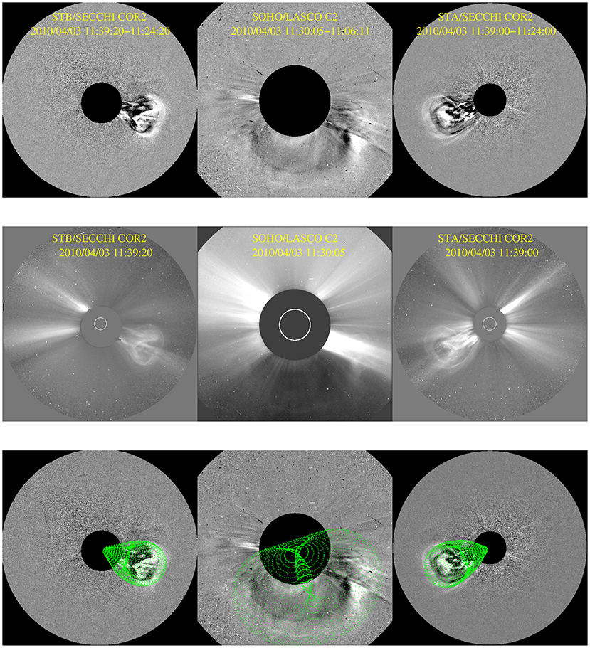
Figure 2. The observation of 3 April 2010 CME from three different viewing angles. The triplet of concurrent images are taken from STEREO/COR2-B (left), SOHO/LASCO-C2 (middle), and STEREO/COR2-A (right) around 11:39 UT on 3 April 2010. The top, middle and bottom panels show the running difference images, direct images, running difference images having GCS model wire-frame overlaid with green, respectively.

FIGURE 3

Figure 3. Same as in Figure 2. In this case, however, the triplet of concurrent images are taken from STEREO/HI1-B (left), SOHO/LASCO-C3 (middle), and STEREO/HI1-A (right) around 15:29 UT on 3 April 2010.

We used the precise measurements of CME's aspect ratio (a) and the height of its leading edge (h), obtained from GCS forward model, to derive the radius of the flux rope as R = $(\frac{a}{1 + a}) h$ . The distance (L) of the center of the flux rope from the solar surface is given as, L = D – 1 R_⊙, where D is the heliocentric distance of the CME's center and is given by, D = h – R. The value of D, R, their first-order time derivative as propagation and expansion speeds (υ_c & υ_e), and their second-order time derivatives as propagation and expansion accelerations (a_c & a_e) are shown in Figure 4. The figure also shows the vertical error bars at each data point considering arbitrary uncertainties of 0.5 R_⊙ and 1 R_⊙ in the measurements of the distance from COR2 and HI1 observations, respectively. The relative uncertainties in the acceleration is larger than that in the speed. This implies that uncertainties in the measurements of R and D will be amplified in its second-order derivatives. Therefore, we smooth the measured D and R before taking their derivatives. In the smoothing process, each observed data point is replaced with the value obtained after a linear fitting of a few neighboring data points within a moving boxcar. The FRIS model involves the acceleration of the CME flux rope and therefore the uncertainties in the measured kinematics of the CME will propagate into the derived model results. In the figure, a measurements gap in the kinematics separates the values derived from COR2 and HI1 observations. The measurement gap appeared because of difficulty in tracking the CME continuously during its transition from the COR2 field of view to the HI1 field of view. Such a situation often arises as CME flux rope becomes faint near the exit edge of COR2 and is not observed as a fully developed structure at the entrance of HI1. The COR2 observations allowed the tracking of the CME from D = 2.5 R_⊙ to 8.6 R_⊙ and the HI1 observations enabled us to track the CME farther from D = 15 R_⊙ to 42 R_⊙ from the Sun. During the evolution of the CME from D = 2.5 to 42 R_⊙, the radius of the flux rope expanded from R = 1.1 to 18.2 R_⊙.

FIGURE 4

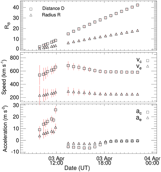
Figure 4. The top panel shows the variations of the heliocentric distance (D) of the center of flux rope CME and its radius (R) with time. The data points before and after the measurements gap correspond to estimates from the COR2 and HI1 observations, respectively. The first-order derivative of D and R as the propagation speed (v_c) and expansion speed (v_e) is shown in the middle panel. The bottom panel shows the propagation acceleration (a_c) and expansion acceleration (a_e) as the first-order derivative of v_c and v_e, respectively. The vertical lines at each data point show the error bars which are derived from the arbitrary assumption of the uncertainties of 0.5 R_⊙ and 1 R_⊙ in the measurements of D from COR2 and HI1 observations, respectively.

From Figure 4, the propagation speed of the CME is found to rise in the beginning from 540 km s⁻¹ at D = 2.5 R_⊙ to 680 km s⁻¹ at D = 15 R_⊙, which slowly declines to be 580 km s⁻¹ at D = 42 R_⊙. Similarly, the expansion speed of the CME flux rope rises from 231 to 293 km s⁻¹ which then smoothly declines to 250 km s⁻¹. We also note a change in the trend of CME acceleration for the measurements in COR2 and HI1. This is possible due to the use of observations from different instruments (i.e., COR2 and HI1) which have different sensitivity, making difficult the tracking of the same feature from COR2 to HI1. However, the deceleration of the CMEs within few solar radii in the coronagraphic field of view, followed by a phase of residual acceleration, has been noted in earlier studies (Zhang and Dere, 2006; Vršnak and Žic, 2007). The effect of tracking uncertainties between COR2 and HI1 may be minimal on the CME thermodynamics which is obtained by the separate run of the FRIS model for the observations of COR2 and HI1, as explained in section 3.3. The kinematics of this CME has also been investigated extensively in earlier studies using different 3D reconstruction techniques on STEREO/COR and HI observations in conjunction with drag based and MHD models (Möstl et al., 2010; Liu et al., 2011; Rollett et al., 2012; Mishra and Srivastava, 2013; Mishra et al., 2014). These studies tracked the density enhanced feature in the shock-sheath region of the CME by constructing the J-maps (Davies et al., 2009). Although our present study derived the kinematics of the CME flux rope using the GCS model instead of tracking the density feature in the J-maps, we find that our estimates of kinematic parameters are in fair agreement to those in earlier studies within 10%. Once the kinematics of the CME flux rope is obtained, it can be used to constrain the FRIS model and probe the internal state of the CME.

3.2. Implementing the FRIS Model

The FRIS model derives the thermodynamic parameters of a CME by using the estimates of the kinematics of the CME, the unknown coefficients (c₁₋₅), and the time-dependent variable λ in the model. To implement the FRIS model, we follow the following three main steps: (i) To determine the best set of unknowns coefficients which can represent the observed characteristics of the flux rope, we fitted the measured values of (L^R²)γ−1 in the left-hand side of Equation (1) with the model derived expression in the right-hand side of the equation. The fitting is performed using MPFITFUN routine of IDL which can fit a user-supplied model to a set of user-supplied measured data (Markwardt, 2009). On using the distance in unit of R_⊙ and time in unit of hr for observed data points of the CME characteristics derived from COR2 observations, the values of the coefficients, i.e., c₁, c₂, c₃, c₄, and c₅ are obtained as 0, −25.6, −75.8, 1.8, and 1.0, respectively. The goodness of the fit can be examined based on the values of (L^R²)γ−1 derived from the measurements (Q_m) and its values derived from fitting (Q_f) model expression. The relative error (δ) in the fitted result compared to the measured results is represented by δ = |Q_m−Q_f|/Q_m, which when multiplied by 100 gives its percentage value. We find that the relative error in the model results to the measurements is always within 10% at any data point in COR2 as shown in Figure 5. This represents a reasonably accurate fitting as the model results match well with the measurements for the selected CME. (ii) We used the obtained values of the coefficients and observed kinematic parameters to determine the value of λ. (iii) Finally, once the values of λ, its derivative, and the coefficients are known, the expressions in Table 1 are used to estimate several thermodynamic parameters of the CME. We note that the obtained values of the coefficients c₁₋₅ are assumed to also represent the evolution of the CME derived from HI observations. Such an assumption helps in mutually comparing the estimates of the CME thermodynamic parameters in COR2 and HI field of view. This is because the estimates of the CME thermodynamic parameters are scaled by the factors involving the coefficients.

FIGURE 5

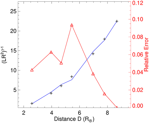
Figure 5. The variations in (L^R²)γ−1 from the measurements (black), the modeled result for this parameter (blue), and the relative error (red) in the model results are shown.

3.3. Thermodynamic Processes in a CME

We examine the evolution of several thermodynamic parameters using the FRIS model for the selected CME of 3 April 2010. The estimated polytropic index, cooling rate, rate of change of entropy, density, temperature, and various forces are shown in Figure 6. It is noted that we could only estimate the absolute value of the polytropic index and rate of change of entropy. The estimates of other parameters are relative values because they are scaled by factors listed in Table 1 and mentioned along the Y-axes of the various panels in the figure. From the top-left panel of the figure, it is found that although there is a small fluctuation in the value of the polytropic index, its value range between 1.7 and 1.9 as the CME is evolving from the inner to the outer corona. Thus, the value of the polytropic index is almost constant during the evolution of the CME. The estimated value of the polytropic index greater than 1.66 implies that CME is releasing the heat into the surrounding.

FIGURE 6

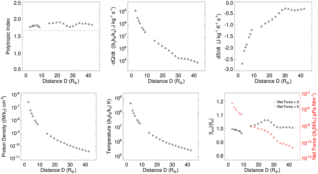
Figure 6. Top: The variation of the polytropic index (Γ), cooling rate (-dQ/dt), and rate of change of entropy (ds/dt) of the CME with the heliocentric distance of the CME's center (D) are shown in the left, central, and right panels, respectively. Bottom: The average proton number density ( $\bar{n_{p}}$ ) and Temperature ( $\bar{T}$ ) of the CME, and different forces acting on the CME with the heliocentric distance of its center (D) is shown in the left, central, and right panel, respectively. The bottom-right panel shows the ratio of absolute values of Lorentz and thermal force ( $| {\bar{f}}_{e m} | / | {\bar{f}}_{t h} |$ ) (on left Y-axis) and the net force (on right Y-axis) acting inside the CME.

The top-central panel of Figure 6 shows that the value of the cooling rate per unit mass (-dQ/dt) which is always positive for the CME of 3 April 2010. However, the value of cooling rate is decreasing continuously as the CME is moving away from D = 2.5 R_⊙ to D = 42 R_⊙. The positive value of cooling rate implies that thermal energy is being released out from the CME into the surrounding. The top-right panel of the figure shows the rate of change of entropy (ds/dt) per unit mass. The value of rate of change of entropy was about –2.7 J kg⁻¹ K⁻¹ s⁻¹ at the beginning of D = 2.5 R_⊙ and continuously increased to become –0.3 J kg⁻¹ K⁻¹ s⁻¹ at D = 42 R_⊙. This implies that the rate of loss of the entropy is getting smaller as the CME is moving away from the Sun. It is also noted that the release of entropy from the CME and its cooling rate are larger near the Sun (i.e, within D = 8.6 R_⊙) than those at larger distances from the Sun.

The bottom-left and bottom-central panels of Figure 6 shows the estimated variations in the average proton density and temperature of the CME with the heliocentric distance of its center, respectively. We note a decrease in average CME density and temperature with the distance which implies a decrease in thermal pressure inside the CME. This is expected as the CME is continuously expanding while moving away from the Sun. The decrease in the proton density and temperature is much faster when the CME is near the Sun (i.e, observed in COR2 within D = 8.6 R_⊙), and the rate of decrease becomes slower tending toward its asymptotic values as the CME moves away from the Sun. This is expected as the expansion acceleration (a_e) is positive (with increase in υ_e from 231 to 283 km s⁻¹) corresponding to COR2 observations and it has negative values (with decrease in υ_e from 293 to 250 km s⁻¹) corresponding to HI1 observed data points (Figure 4).

As described in section 3.2, the value of the coefficient c₁ is estimated to be zero from the fitting of Equation (1). c₁ is related to the poloidal motion of the plasma, and thus the centrifugal force is found to be absent for the CME of 3 April 2010. This is expected as there is no strong evidence of significant poloidal motion in CMEs near the Sun. However, recent works has suggested the presence of poloidal plasma motion inside the CMEs near 1 AU possibly due to local mechanisms rather than a global cause (Wang et al., 2015; Zhao et al., 2017a,b). In the present study, we found that the dynamics of the selected CME is governed by the Lorentz force ( ${\bar{f}}_{e m}$ ) and thermal pressure force ( ${\bar{f}}_{t h}$ ). The evolution of the ratio of the absolute value of average Lorentz to thermal forces and the net force ( $\bar{f}$ ) inside the CME is shown in the bottom-right panel of Figure 6. From the figure, it can be noted that the ratio of the two forces is slightly smaller than unity near the Sun (i.e, within D = 8.6 R_⊙) while it becomes slightly larger than unity at larger distances from the Sun in HI1 field of view. Thus, the magnitude of the thermal force is larger than the Lorentz force near the Sun. The net force inside the CME (i.e., Lorentz force + thermal pressure force) is found to be positive near the Sun, within D = 8.6 R_⊙, after which the net force is negative at a larger distance. This implies that the directions of the two forces are opposite. Further, it is noted from Figure 4 that the expansion acceleration is positive (i.e., a_e = 3–11 m s⁻²) below D = 8.6 R_⊙ and beyond this distance its value becomes negative (i.e., a_e = −2.3 to −0.2 m s⁻²). Thus, we find that the Lorentz force ( ${\bar{f}}_{e m}$ ) acting toward the center of the CME prohibits it from free expansion. The thermal pressure force ( ${\bar{f}}_{t h}$ ) acting away from the center of the CME is the actual internal cause of the CME expansion. It is evident that the absolute values of both the ${\bar{f}}_{e m}$ and ${\bar{f}}_{t h}$ forces are getting very close to each other at the last few data points where the expansion acceleration is also close to zero.

4. Extrapolation of CME Internal State Up to 1 AU

4.1. Estimation of CME Kinematics

The internal thermodynamic parameters of the CME can be estimated up to 1 AU if the measured propagation and expansion speed profiles of the CME to be used as inputs in the FRIS model (Mishra and Wang, 2018) could be measured up to 1 AU. However, we could not unambiguously identify CME flux rope using GCS forward fitting model (Thernisien et al., 2009) beyond D = 42 R_⊙, as explained in section 3.1. To derive the CME speed from the distances beyond D = 42 R_⊙ to near the Earth at L1, we implemented the drag based model (DBM) (Vršnak et al., 2013). The DBM assumes that beyond a distance of 20R_⊙, the acceleration of a CME is governed by the interaction between the CME and the ambient solar wind via aerodynamic drag (Cargill, 2004). The quadratic form of the instantaneous drag acceleration is, a_d = −K_d (v−w) |(v−w)|, where v, w, and K_d are the instantaneous speed of the CME, ambient solar wind speed, and the drag parameter, respectively. The analytical solution to the equation of motion of a CME under the drag acceleration with the approximation of K_d(r) = constant and w(r) = constant, can be written as Equation (2). In the equation, the sign ± depends on deceleration/acceleration regime, i.e., it is plus for υ₀ > w, and minus for υ₀ < w.

\begin{array}{l} r (t) = \pm \frac{1}{K_{d}} ln [1 \pm K_{d} (υ_{0} - w) t] + w t + r_{0} & (2) \end{array}

From Equation (2), we can find the time taken by a CME to travel from an initial radial distance (i.e., r₀ at t= t₀) to a final distance (i.e., r at t) for a given initial take-off speed of υ₀. The estimation of the drag parameter (K_d) for an individual CME depends on the cross-sectional areas of CME, solar wind density and CME mass. The large uncertainties in the estimation of the CME mass using coronagraphic observations from single and multiple viewpoints has been discussed in earlier studies (Vourlidas et al., 2000; Colaninno and Vourlidas, 2009; Mishra et al., 2014). Because of the limited accuracy in the estimation of variables on which the drag parameter depends, we take its value from a statistical study of a large number of events in Vršnak et al. (2013).

The study of Vršnak et al. (2013) shows that the drag parameter (K_d) often lies in the range 0.2 × 10⁻⁷ to 2.0 × 10⁻⁷ km⁻¹. They also showed that the ambient solar wind speed should be chosen to lie between 300 and 400 km s⁻¹ for a slow solar wind environment, and between 500 and 600 km s⁻¹ for fast solar wind environment created by a coronal hole in the vicinity of the source region of the CME. We note that the study of Vršnak et al. (2013) represents the drag parameter with the symbol γ while we have reserved this symbol for the adiabatic index. The selected CME is propagating at least partly through a high-speed solar wind stream as confirmed in earlier studies (Möstl et al., 2010; Liu et al., 2011; Rollett et al., 2012). For such cases, it is suggested in Vršnak et al. (2013) that a higher value of the solar-wind speed should be combined with a lower value of drag parameter. In this way, we took a straightforward option to choose the drag parameter and extrapolate the CME kinematics beyond the HI field-of-view where the CME could not be tracked unambiguously.

The Earth was found to be immersed in high-speed solar wind from a coronal hole located at a geoeffective location on the Sun during the arrival of this CME at 1 AU. It is most likely that high-speed wind has partly influenced the kinematics of this fast CME. Several studies have established the moderate deceleration of a CME during its journey from the Sun to 1 AU because of aerodynamic drag by the ambient high-speed (Möstl et al., 2010; Liu et al., 2011; Rollett et al., 2012; Mishra and Srivastava, 2013). In such a case, we extrapolated the obtained kinematics of the CME from GCS fitting (Figure 4) up to 1 AU by implementing the DBM (Vršnak et al., 2013). Using the last data point from GCS fitting, we find the heliocentric distance of the leading edge (i.e., h = D + R) of the CME at 60.5 R_⊙ with the speed (i.e., propagation speed + expansion speed) of 830 km s⁻¹ at 22:10 UT on 3 April 2010. These characteristics of the CME leading edge such as radial distance, speed and time are used as initial inputs in Equation (2). Further, we used a high value of w= 550 km s⁻¹ combined with a low value of K_d = 0.2 × 10⁻⁷ as the high-speed solar wind is characterized by low density and high speed. Once the time variations of h is estimated, we derived other kinematic parameters up of the CME up to 1 AU (Figure 7) to be used in the FRIS model. To estimate the values of R corresponding to h, it is assumed that the aspect ratio (a) of the CME flux rope remains the same as derived from the GCS model using COR2 observations. The validity of the assumption of constant aspect ratio is discussed in section 5.

FIGURE 7

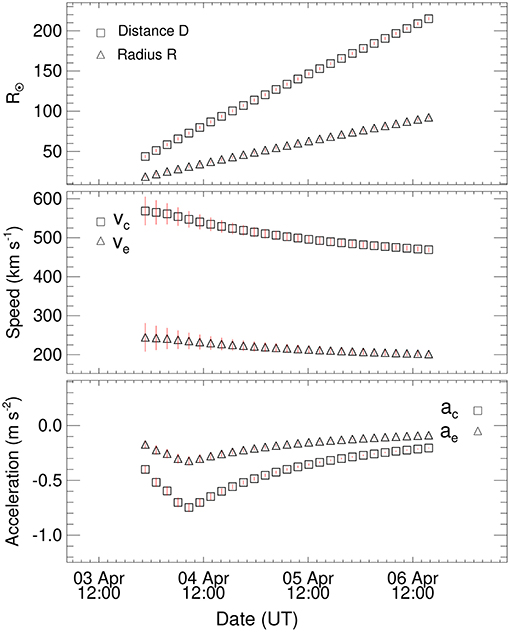
Figure 7. The kinematics of 3 April 2010 CME as obtained by using the drag based model (DBM) is shown. Top panel shows the estimated heliocentric distances (D) of the center of flux rope CME and its radius (R). The first-order derivative of D and R as the propagation speed (v_c) and expansion speed (v_e), respectively, are shown in the middle panel. The bottom panel shows the propagation acceleration (a_c) and expansion acceleration (a_e) as the first-order derivative of v_c and v_e, respectively. The vertical lines at each data point show the error bars. The errors are derived from the arbitrary assumption of the uncertainties of 2 R_⊙ in the estimates of D.

The estimates of kinematics for the CME using the DBM from D = 44 R_⊙ to 1 AU is shown in Figure 7. From the figure, it can be seen the estimated arrival time of the center of the CME flux rope at L1 at about 15:30 UT on 6 April with a transit speed (υ_c) of 470 km s⁻¹. At this distance, the radius of the flux rope is 90 R_⊙ having an expansion speed (υ_e) of 200 km s⁻¹. From the obtained latitude and longitude of the CME using GCS model in section 3.1, the CME is found to be heading toward the Earth, and an interplanetary counterpart of the CME should be observed by the spacecraft near the Earth. Using the in situ observations taken by WIND spacecraft (Ogilvie et al., 1995), Figure 14 in Mishra and Srivastava (2013) shows the arrival of a CME at the L1 point as a magnetic cloud (Klein and Burlaga, 1982; Lepping et al., 1990). Since the magnetic cloud is known to be a flux rope structure, the observed properties of the magnetic cloud can be compared with the properties of the flux rope estimated from the DBM as it will be explained in section 5. Once we could estimate the propagation and expansion characteristics of the CME up to 1 AU, they can be used as inputs in the FRIS model to extrapolate the CME thermodynamic parameters.

4.2. Estimation of CME Thermodynamics

We used the expressions from Table 1 and derived the CME thermodynamic parameters which are shown in Figure 8. It is noted that the value of the fitted coefficients (i.e., c₁₋₅) as used with COR2 and HI observed CME parameters are assumed to represent the evolution of the CME estimated from the DBM. From the top-left panel of Figure 8, it is seen that the polytropic index of the CME plasma remains constant at about 1.9 up to the moment the center of the CME reached 1 AU. The value of the polytropic index implies that the CME is continuously releasing heat into its surrounding during its heliospheric journey up to near the Earth. From the top-central panel of the figure, it is clear that the cooling rate (i.e, heat release out from the CME) is much faster at a smaller distance and becomes slower at the distances larger than D = 80 R_⊙. The top-right panel shows that there is a loss of entropy (i.e., the release of entropy) from the CME throughout its heliospheric journey. However, the rate of loss of entropy became smaller beyond the distance D = 80 R_⊙.

FIGURE 8

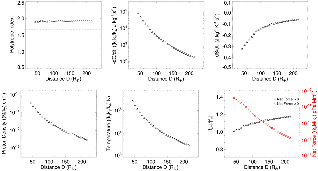
Figure 8. Top: The variation of the polytropic index (Γ), cooling rate (-dQ/dt), and rate of change of entropy (ds/dt) of the CME with the heliocentric distance of the CME's center (D) is shown in the left, central, and right panels, respectively. Bottom: The average proton number density ( $\bar{n_{p}}$ ) and Temperature ( $\bar{T}$ ) of the CME, and different forces acting on the CME with the heliocentric distance of its center (D) is shown in the left, central, and right panel, respectively. The bottom-right panel shows the ratio of absolute values of Lorentz and thermal force ( $| {\bar{f}}_{e m} | / | {\bar{f}}_{t h} |$ ) (on left Y-axis) and the net force (on right Y-axis) acting inside the CME.

The bottom-left panel of Figure 8 shows the decrease in the average proton density of the CME implying its continuous expansion up to 1 AU. The expansion is seen from the middle panel of Figure 7. The bottom-central panel of Figure 8 shows a decrease in the average temperature of the CME implying the work done by the CME in the process of expansion. The result suggests that the CME originated from hotter source region on the Sun and cools down during its expanding propagation. Looking Figures 6, 8 together, we note that the decrease of density and temperature of the CME is faster at lower distances and tends toward its asymptotic values. Our analysis suggests that the expansion of the CME has not been sufficient before the CME reaches the Earth and, therefore, the CME is found to release heat and entropy into the surrounding.

The bottom-right panel of Figure 8 shows the ratio of absolute values of the Lorentz ( $| {\bar{f}}_{e m} |$ ) to thermal pressure forces ( $| {\bar{f}}_{t h} |$ ) and the net force acting inside the CME. From the figure, we note that the value of $| {\bar{f}}_{e m} | / | {\bar{f}}_{t h} |$ is around 1.01 in the beginning at D= 44 R_⊙ and increases slowly to become around 1.17 at D= 1 AU. We also note that the net force which is the vector sum of Lorentz and thermal pressure force is always negative from D= 44 R_⊙ to 1 AU. It implies that the Lorentz force is larger in magnitude than the thermal pressure force, and the direction of both the forces are opposite to each other. The Lorentz force prohibiting the free expansion of the CME leads to the expected negative net force which also corresponds to the negative expansion acceleration of the CME as shown in the bottom panel of Figure 7.

4.3. Comparison of Model Results With in situ Observations at 1 AU

The selected CME in our study is found to arrive at Earth and its identification in the in situ observations at the L1 point has been made in earlier studies (Möstl et al., 2010; Mishra and Srivastava, 2013). Using the FRIS model, in the present study, we could estimate the absolute value of the rate of change of entropy (ds/dt). The absolute value of heating rate per unit mass of the CME plasma can be written as, dQ/dt= ds/dt × T, where T is the average temperature of the CME plasma. Thus, the absolute value of the heating rate per unit mass of the CME plasma can also be estimated if the real temperature was known. Figure 14 in Mishra and Srivastava (2013) shows that the selected CME is identified as a magnetic cloud near the Earth and its average temperature [i.e., (T_p+T_e)/2] is noted as 4 × 10⁴ K. The value of rate of change of entropy obtained from FRIS model at D= 1 AU is −5.8 × 10⁻² J kg⁻¹ K⁻¹ s⁻¹. Therefore, the absolute value of heating rate of the CME plasma at D= 1 AU is estimated as −2.3 × 10³ J kg⁻¹ s⁻¹. The negative value of heating rate implies the cooling, i.e., the release of heat from the CME. The release of thermal energy from the CME is also confirmed from the value of the polytropic index which is about 1.9 at D= 1 AU.

Using the FRIS model, the average temperature of the CME at 1 AU is estimated as 3.17 × 10³ K with a scale factor of k₂k₈/k₄. From the in situ observations, the average temperature of the CME near 1 AU is noted as 4 × 10⁴ K. On comparing the model-derived temperature with in situ observed temperature, the value of the factor k₂k₈/k₄ is estimated as 12.6. The value of the factor depends on the coefficients c₁₋₅ fitted from the model which is assumed to be the same during the entire journey of the CME. Therefore, if the value of the factor k₂k₈/k₄ is assumed to be the same near the Sun as at 1 AU, the temperature of the CME would be 10⁹ K at the distance of a few solar radii from the Sun. Clearly, the FRIS model overestimates the temperature near the Sun while underestimated its value near the Earth.

Further, it is evident from Table 1 that if the absolute value of the proton number density is obtained by other means independent of the model, one can derive the unknown factor M/k₇. In this factor, M is the mass of the CME and k₇ is an important proportionality constant between the axial length (l) of the flux rope and the distance of the center of the flux rope from the solar surface, i.e., l = k₇ L, as derived in Mishra and Wang (2018). The model derived the proton number density of the CME at 1 AU is 3.09 × 10⁻¹³ × M/k₇ cm⁻³ while the in situ observed proton density of the magnetic cloud is 2 cm⁻³. On comparing the model derived and observed density, the value of the factor M/k₇ is found as 6.4 × 10¹² kg. The value of true mass (M) for the CME of 3 April 2010 is estimated as 3.16 × 10¹² kg in an earlier study of Bein et al. (2013). This mass is estimated using the method developed by Colaninno and Vourlidas (2009) where they use the two viewpoints of STEREO. From the mass estimates, the value of k₇ is estimated as around 0.5 which is too small to be realistic. In fact, the value of k₇ is found to be around 2.57 in earlier studies (Wang et al., 2015, 2016).

The small value of k₇ suggests the underestimation of the proton number density from the FRIS model near 1 AU and/or underestimation of CME mass. The underestimation of CME mass by a factor of two is noted in the mass estimation method which assumes the CME propagating in the plane of sky of the observer (Vourlidas et al., 2000). In the mass estimation method using coronagraph observations from multiple viewpoints of STEREO (Colaninno and Vourlidas, 2009), one can find the 3D direction of CME improving on the plane of sky assumption but still, the true width of the CME along the line of sight remains unknown. This unknown width of the CME and assumption that CME mass lies in a plane can lead to an underestimation of CME mass by up to 15% (Vourlidas et al., 2000). We also note that while comparing the model results with the observations at 1 AU, we used the mass estimates from near-Sun coronagraph observations. However, far from the Sun, the measured CME mass is found to increase due to piled-up mass of solar wind plasma around the CME, called the snow plough effect (Tappin, 2006; DeForest et al., 2013). We think that the extrapolation of CME thermodynamic parameters up to a large distance from the Sun, i.e., 1 AU have larger uncertainties due to limited accuracy in the input parameters of the model. Further insight can be made if the in situ observations of CME density and temperature are derived at other closer distances from the Sun. Further, we can see from Table 1 that if the constant k₂ can be obtained, the absolute value of forces acting inside the CME can be estimated. The present study did not discuss each constant but rather focused on demonstrating the potential of the FRIS model for estimating the thermodynamic parameters of the CME from the Sun to 1 AU.

5. Results and Discussion

Our present study estimates the thermodynamic parameters of the 3 April 2010 CME from near the Sun to the Earth using the Flux rope internal state (FRIS) model. Thus the model is efficient in probing the CME internal state at distances often inaccessible by the in situ spacecraft which usually provide the information on CME thermodynamics. The input for the model is the estimated kinematics of the CME which is derived using the SOHO/LASCO and STEREO/COR white-light observations in combination with the drag based model (DBM). The white-light observations enabled the identification of the CME flux rope to be fitted from the GCS model from D = 2.5 to 42 R_⊙, and thereafter the DBM is used up to D = 1 AU. The estimated thermodynamic parameters of the CME is shown in Figures 6, 8. From both figures, we note that the polytropic index of the CME plasma ranged between 1.7 and 1.9 up to D = 42 R_⊙, and beyond this distance, the value of polytropic index remains constant as 1.9 up to D = 1 AU. A value of the polytropic index greater than 1.66 suggests that there is a release of heat out from the CME throughout its journey from near the Sun to Earth.

The obtained value of the polytropic index is not in agreement with earlier studies of Liu et al. (2006a) where they have reported a value of the polytropic index ranging between 1.1 and 1.3. However, they used in situ observations of ICMEs between 0.3 AND 20 AU and derived their result statistically. In a recent study, using the FRIS model, Mishra and Wang (2018) shows that the polytropic index for a CME (12 December 2008 event) decreases from 1.8 to 1.3 between D = 6 and 15 R_⊙. We, in the present study, find no systematic variation in the polytropic index despite tracking the CME up to much larger distances. It means that the CME of 3 April 2010 is always in heat releasing state unlike the CME shown in Mishra and Wang (2018) that was initially releasing heat before reaching an adiabatic state and then started acquiring heat from the ambient medium. We note that the CME of 12 December 2008 was having a slower speed while the CME selected for the present study is a fast CME showing only a moderate deceleration from the Sun to 1 AU. The moderate deceleration of the CME is expected as it is being pushed from the back by the high-speed wind which contributed to the CME's propagation speed but prohibited the CME from expansion. It has been shown that an interaction between the high-speed stream and the preceding magnetic cloud can compress the preceding structure (Fenrich and Luhmann, 1998; Gopalswamy et al., 2009). Thus, the insufficient expansion might not have allowed the CME to be cool enough to depart from the heat releasing state to an adiabatic state with the ambient surrounding.

It is expected that the heating of plasma in the open magnetic field configuration of the solar wind and in the closed magnetic field configuration of CMEs would be different. Thus, it is interesting to compare the magnitude of the estimated polytropic index of the selected CME with that of the solar wind plasma. The estimation of the polytropic index for the solar wind has been the subject of many studies (Parker, 1960; Feldman et al., 1978; Sittler and Scudder, 1980; Totten et al., 1995; Nicolaou et al., 2014). In the polytropic solar wind theory of Parker (1960), the polytropic index is suggested to be smaller than 1.5 to obtain an accelerated wind solution. This implies that the solar wind acceleration would become negative for the value of the polytropic index larger than 1.5, and no real wind-type solution exists. In Feldman et al. (1978) study, the value of electron polytropic index was determined to be 1.45 while Sittler and Scudder (1980) obtained its empirical value to be as 1.18. Further, Totten et al. (1995) empirically estimated the proton polytropic index and found its value to be 1.46. Recently, Nicolaou et al. (2014) determined that the average value of proton polytropic index to be around 1.8. Thus, there are mutually differing results on the behavior of solar wind whether it is more like that of an isothermal gas than an adiabatic one. In our study, the polytropic index of the ICME is around 1.8 which is clearly larger than the value for solar wind reported in most of the earlier studies. However, we expect that the selected Earth-directed CME of 3 April 2010 to be a unique case which is continuously being pushed by the high-speed stream emanating from a coronal hole located at a geoeffective location on the Sun (Möstl et al., 2010; Liu et al., 2011).

From the ratio of Lorentz and thermal pressure forces and the resultant direction of the net force as shown in Figures 6, 8, it is evident that the Lorentz force is acting toward the center of the CME flux rope while the thermal pressure force is acting away from the center. The magnitude of both forces decreases as the CMEs moves out away from the Sun, however, the decrease in thermal pressure force is faster than the Lorentz force. This is evident as the net force is acting outward from the CME center in the beginning before D = 8.6 R_⊙ and beyond this distance, the net force is found to have the direction toward the center of the CME. Further, the expansion acceleration has the positive value (a_e > 0) before D = 8.6 R_⊙ and after its value becomes negative (a_e < 0). The consistency in the direction of the net force and expansion acceleration suggests that the thermal pressure drives the expansion of the CME while the Lorentz force prohibits the CME from expansion. The direction of the Lorentz force is decided by the distribution of the B_z in the cross-section of the CME flux rope as described in Mishra and Wang (2018). The ratio of the magnitude of the Lorentz to thermal force is ranging between 0.99 and 0.96 before D = 8.6 R_⊙, and beyond this distance it ranges between 1.01 and 1.17. This clearly shows that even a small difference between these two forces can change the expansion acceleration by a few m s⁻². Surprisingly, the CME is found to be in heat releasing state throughout its journey irrespective of the sign of the expansion acceleration and the net force.

In the process of heat release from the CME, we note a loss of entropy during the propagation of the CME from the Sun to Earth. The rate of loss of entropy is −2.7 J kg⁻¹ K⁻¹ s⁻¹ at D = 2.5 R_⊙ which reduced to be −0.58 J kg⁻¹ K⁻¹ s⁻¹ at D = 1 AU. The rate of loss of the entropy is much faster before D = 8.6 R_⊙ when the expansion acceleration and the net force are found to be positive. The cooling rate of the CME is consistent with the rate of loss of entropy throughout the CME journey. This is possible if the CME has higher heat content than the surrounding medium due to its compression by the high-speed wind stream from behind. We would like to point out that because of simplicity, the polytropic law has been employed in several studies. However, the polytropic approximation is a gross simplification of the real energy transport equation. There are various processes such as turbulence, magnetic field dissipation, conduction of heat from solar atmosphere, heat exchange with ambient medium, etc. which can lead to heating/cooling of the CMEs. Thus, using the FRIS model, the identification of the process responsible for the reported cooling of the CME remains unsolved, and further studies are required in this direction.

Interestingly, the CME is identified as a magnetic cloud in in situ observations at L1. The center of the magnetic cloud arrived at 02:50 UT on 6 April 2010 preceded by the arrival of a shock at 8:28 UT on 5 April 2010. The magnetic cloud, from its leading to trailing edge, took around 26.4 hr to cross the L1 point. The average propagation speed (υ_c) of the cloud is observed as 650 km s⁻¹ while its expansion speed (υ_e) as 115 km s⁻¹ at L1. From the in situ observed speeds at L1, the aspect ratio of the CME is measured to be around 0.20 which is around half of the aspect ratio derived from the GCS model on COR2 and HI-1 observations. It is clear that our assumption of constant aspect ratio for the CME, beyond the HI-1 observed last data point, breaks down before its arrival at L1. It is expected that the assumption would be broken gradually as the CME propagates away from the Sun in the radially expanding solar wind. Because of this, the estimates of radius, expansion speed, and expansion acceleration, determined using the combination of aspect ratio and heights of the CME obtained from DBM, would also have uncertainties. A correction factor to the aspect ratio of the CME, based on the near-Sun and near-Earth observations of the CME, may be introduced for examining its time variation. In another study, we plan to estimate the uncertainties in the thermodynamic parameters derived from the FRIS model due to uncertainties in the expansion characteristics which is used as inputs in the model.

From the in situ observations at L1, the radius of the cloud is measured to be around 89 R_⊙. The observed arrival time of the center of the cloud at L1 is around 12.6 hr early than estimated from DBM in section 4.1. Although the estimates of the radius of the cloud from the DBM and in situ observations are almost equal, the DBM estimates of propagation and expansion speed are 180 km s⁻¹ smaller and 90 km s⁻¹ larger, respectively, than the observed values. The underestimation of the propagation speed of the CME flux rope (i.e., magnetic cloud) from the DBM is consistent with the estimation of its delayed arrival near the 1 AU. However, the overestimation of expansion speed from the DBM may arise because of neglecting the flattening of the CME's front (i.e., constant aspect ratio assumption), the interaction of the CME with the high-speed wind, and/or trajectory of in situ spacecraft through the flank of the magnetic cloud (Möstl et al., 2010). It appears that when compressing a CME by high-speed wind from its back, the radial extent of the CME may not decrease but its expansion may slow down. This is most likely if the compression happens for a certain duration after which the CME may overexpand to return to its expected size.

It is also noted that the drag-based model assumes that the CME is propagating into an isotropic ambient solar wind. However, the CME has a 3D structure spanning over different longitudes and latitudes. Therefore, it is possible that parts of the CME at different latitudes and longitudes are influenced by solar wind of different speeds. It is expected that the high-speed wind from coronal holes may strongly affect the part of the CME at higher latitudes than that at lower latitudes (Heinemann et al., 2019). The CME can also experience solar wind of different speeds during the different segments of its heliospheric journey (Temmer et al., 2012; Mishra et al., 2014). However, the drag-based model employed in our study using a typical value for solar wind speed has been validated (Vršnak et al., 2013) to estimate the CME arrival time with typical errors of only around 0.5 day which can be further reduced by improving the drawbacks of the simplified drag-based model. Thus,the effect of several assumptions in the DBM (Vršnak et al., 2013), FRIS model (Mishra and Wang, 2018), and the observational path of the in situ spacecraft is not evaluated in the present study.

The cooling rate of the CME is found to change by an order of 10⁶ during its propagation from near the Sun to 1 AU. We also note that the density and temperature of the CME changed by an order of 10⁵ from near the Sun to 1 AU. It seems that the FRIS model overestimates the value of temperature near the Sun while underestimates near the Earth. This may arise if the measured expansion acceleration is overestimated near the Sun and underestimated at far distances. The values obtained from the FRIS model need further verification from the observations at different distances from the Sun. We expect that the in situ observations from Parker Solar Probe (PSP) and upcoming Solar Orbiter (SolO) would help to understand CMEs parameters at various distances by repeatedly probing the region closer to the Sun. The measurements of CME electron density at various distances from the Sun using polarimetric remote sensing observations can help to validate the model results. Thus, a comparison of results from independent methods has the potential to better interpret the evolution of the CME thermodynamics. We also emphasize that some of the unknown constants in the FRIS model can be constrained to a reasonable value if some properties (e.g., density, temperature, etc.) of the CMEs are measured independently at different distances from the Sun.

We note that there have been observations that proton temperature in a direction perpendicular (T_⊥p) to the magnetic field is larger than that parallel (T_∥p) to the field in the region of ICMEs sheath, solar wind, and planetary magnetosheath (Marsch et al., 1982; Fuselier et al., 1994; Liu et al., 2006b). Such a temperature anisotropy, i.e., T_⊥p/T_∥p > 1, is found to be a direct consequence of the magnetic field line draping and plasma depletion in planetary magnetosheaths and around a fast ICMEs driving a shock (Crooker and Siscoe, 1977; Gosling and McComas, 1987). The anisotropic ion distributions exceeding certain thresholds for instabilities may induce proton cyclotron waves and mirror mode waves in ICMEs sheath, but unlikely inside the ICMEs characterized by low plasma beta (Gary, 1992; Liu et al., 2006b; Ala-Lahti et al., 2018). The heating effects of these waves are not investigated in our study, rather we assumed an average plasma temperature and pressure for describing the CME thermodynamic evolution.

Furthermore, since the FRIS model incorporates the total pressure from electron and proton populations in terms of expansion speed of the flux rope, it is worth comparing the polytropic index from FRIS model to the estimates of proton and electron polytropic index from in situ observations at a specific distance from the Sun. The electron polytropic index is often reported to be smaller than unity (Γ~0.5) while the proton polytropic index is larger than unity (Γ~1.2) in CMEs (Osherovich et al., 1993; Sittler and Burlaga, 1998). This implies that energy transport for the electrons and protons can be approximated by two different polytropes. However, it is complex to understand the electron polytropic index because of the core and halo components and their anisotropy. The solar wind electron characteristics inside and outside CMEs have been investigated in earlier studies (Sittler and Burlaga, 1998; Skoug et al., 2000). Future studies in this direction would be relevant as the energy transport (thermal equilibrium and evolution) for the electrons from the Sun may be more effective than that of the protons for the same temperature.

The mass of the CME is an input parameter in the FRIS model as the expressions for thermodynamic parameters (e.g., density, forces, etc.) have scaling factors involving the CME mass and other unknown constants (Table 1). The mass of the CME also partly contributes to the value of the drag parameter used in the drag-based model of CME propagation. Thus, the CME's mass, the estimation of which involves large uncertainties (Vourlidas et al., 2000; Colaninno and Vourlidas, 2009), can influence the thermodynamic and kinetic evolution of the CME. However, in our study, we showed the trend of variation in the derived thermodynamic parameters instead of deriving their absolute magnitudes. Further, we did not estimate a specific value of drag parameter for the selected CME rather we used its value as suggested by Vršnak et al. (2013) based on a statistical sample of events. Therefore, we did not require the exact magnitude of CME mass in our study to find the trend of variations in the density and forces as shown in Figures 6, 8 with scaling factors.

It is known that CMEs interacts with the solar wind during its heliospheric propagation. Such interaction leads to momentum exchange between the CME and solar wind due to drag force (Cargill et al., 1996), restricts the free expansion of the CME due to solar wind pressure (Klein and Burlaga, 1982), and causes flattening or pancaking of the CME due to solar wind stretching effect (Riley and Crooker, 2004). The FRIS model indirectly includes solar wind drag force and restricting effect on expansion by indirectly measuring the distance of CME flux rope (L) and the radius (R) of its cross-section. However, the solar wind stretching effect by radially expanding solar wind which distorts the circular cross-section of the flux rope is not taken into account in our model. This implies that in our study radius and expansion speed of the CME is overestimated while the distance of CME flux rope from the Sun and propagation speed is underestimated. Since these kinematic parameters of the flux rope are used as inputs in the model, we admit that the model results are affected by the assumptions on the flux rope structure. The extent of underestimation and overestimation would be increasingly larger at distances away from the Sun as the distortion of the CME flux rope is less severe at smaller distances. The effect of this as an underestimation of thermal pressure and Lorentz force is discussed in earlier studies (Wang et al., 2009; Mishra and Wang, 2018). Further, the FRIS model has not considered the curvature of the axis of the flux rope and thus an additional component of Lorentz force driving the CME is neglected. This would further cause an underestimation of the Lorentz force from the model.

Also, the FRIS model assumes a self-similar expansion for the CME during its propagation. This assumption breaks gradually as the CME moves away from the Sun and its obvious evidence is flattening of CME due to solar wind stretching effect (Riley and Crooker, 2004). However, it has been suggested that the self-similar expansion of CMEs remains a valid approximation when the CME is nearly force-free and within tens of solar radii from the Sun (Low, 1982; Chen et al., 1997; Démoulin and Dasso, 2009; Subramanian et al., 2014). Thus, we emphasize that the uncertainties in model thermodynamic parameters may come from the assumptions in the FRIS model and also from the uncertainties in the CME measurements. The extent of such uncertainties would be different at different distances from the Sun and their evaluation require a separate in-depth study. The present study focused on extrapolating the thermodynamic parameters of 3 April 2010 CME from near the Sun to 1 AU, and shows the potential of FRIS model. The findings from the present study regarding the evolution of CME internal state is in contrast to earlier studies (Liu et al., 2006a; Mishra and Wang, 2018). Therefore, using the FRIS model, it is worth examining several cases of CMEs having different kinematic characteristics to better understand the physical processes responsible for the thermodynamic evolution of the CMEs.

We finally note that the kinematics of the CME derived from the methods such as the GCS forward fitting model (Thernisien et al., 2009) and drag-based model (DBM) (Vršnak et al., 2013) would also have some uncertainties. This is possible because of an ideal assumption of graduated cylindrical shell geometry for flux rope structure in the GCS fitting model and negligence of Lorentz force in the DBM. The uncertainties in the kinematics would lead to further uncertainties in the thermodynamic parameters derived from the FRIS model, even if all the assumptions in the FRIS model is found to be perfectly valid. To assess the effect of these uncertainties, it would require to re-run the FRIS model corresponding to new kinematic profiles accounting for the error bars therein. The re-run of the FRIS model means the estimation of a new set of fitting coefficients introduced in the model by fitting the observations with the model derived expressions. Based on our attempts, we find that the new fitting coefficients would be completely different due to the highly non-linear and sensitive fitting equation involved in the FRIS model. Since the model derived thermodynamic parameters are scaled by the fitting coefficients, the estimated thermodynamic parameters using completely different sets of coefficients cannot be directly compared with each other. However, we plan to tackle this issue and perform a separate in-depth analysis assessing the effects of the uncertainties in CME kinematics on the thermodynamic evolution of the CME.

Data Availability Statement

The datasets generated for this study are available on request to the corresponding author.

Author Contributions

WM and YW contributed to the initial conception of the paper. WM wrote the main draft having discussion on analysis with LT, JZ, and YC. All of the authors have read the paper and approved its final version.

Funding

YW is supported by the National Natural Science Foundation of China (NSFC) grant nos. 41574165, 41774178, and 41761134088.

Conflict of Interest

The authors declare that the research was conducted in the absence of any commercial or financial relationships that could be construed as a potential conflict of interest.

Acknowledgments

We acknowledge the UK Solar System Data Center (UKSSDC) for providing the STEREO/COR2 and HI data.

References

Akmal, A., Raymond, J. C., Vourlidas, A., Thompson, B., Ciaravella, A., Ko, Y.-K., et al. (2001). SOHO observations of a coronal mass ejection. Astrophys. J. 553, 922–934. doi: 10.1086/320971