 Robert A. Marshall
 Wei Xu
 Antti Kero2
 Ennio Sanchez
94% of researchers rate our articles as excellent or good
Learn more about the work of our research integrity team to safeguard the quality of each article we publish.
Find out more
ORIGINAL RESEARCH article
Front. Astron. Space Sci., 19 February 2019
Sec. Space Physics
Volume 6 - 2019 | https://doi.org/10.3389/fspas.2019.00006
This article is part of the Research TopicActive Experiments in Space: Past, Present, and FutureView all 21 articles
We present numerical simulations and analysis of atmospheric effects of a beam of 1 MeV electrons precipitating in the upper atmosphere from above. Beam parameters of 100 J or 1 kJ injected in 100 ms or 1 s were chosen to reflect the current design requirements for a realistic mission. We calculate ionization signatures and optical emissions in the atmosphere, and estimate the detectability of optical signatures using photometers and cameras on the ground. Results show that both instruments should be able to detect the beam spot. Chemical simulations show that the production of odd nitrogen and odd hydrogen are minimal. We use electrostatic field simulations to show that the beam-induced electron density column can enhance thunderstorm electric fields at high altitudes enough to facilitate sprite triggering. Finally, we calculate signatures that would be observed by incoherent scatter radar (ISR) and subionospheric VLF remote sensing techniques, although the latter is hindered by the limitations of 2D simulations.
Electron guns firing artificial beams of electrons with energies in the tens of keV have been used since the 1970s to probe magnetospheric and auroral physics (e.g., Winckler, 1980; Neupert et al., 1982; Burch et al., 1993; Stone and Bonifazi, 1998). In the late 1980s, the idea of using a relativistic beam of electrons took hold (e.g., Banks et al., 1987, 1990); a comprehensive review of research into relativistic beam experiments up to 1992 was provided by Neubert and Banks (1992). Relativistic (MeV) beams have a variety of advantages over keV beams, including beam stability and reduced spacecraft charging effects (Neubert and Gilchrist, 2002), and faster propagation along magnetic field lines (Delzanno et al., 2016; Dors et al., 2017). Krause (1998) performed detailed calculations of the atmospheric response to a relativistic electron beam, including calculations of beam dynamics and stability, and ionization and X-ray production in the atmosphere. Further calculations were made by Neubert et al. (1996) on the propagation of the electron beam in the magnetosphere and the atmospheric response.
In recent years we have begun exploring a number of potential applications of space-based, artificial relativistic beam injection, including magnetic field line mapping, studies of wave-particle interactions, and studies of the atmospheric effects of precipitation, that should be enabled by the present state of technology in particle accelerators. However, any such experiment relies on the ability to detect and measure the beam, either in-situ by directly observing the electron beam, or by remote sensing from the ground, by observing the atmospheric signatures of the beam precipitating in the atmosphere. For the latter, we need to assess the diagnostic signatures of the beam in the atmosphere.
Marshall et al. (2014) expanded on the work of Krause (1998) to calculate optical emissions observable from the ground, X-ray production and propagation and detectability from satellites and balloons, and backscattered electrons that could be observed from Low Earth Orbit (LEO). That study showed that optical signatures are likely detectable; indeed, the SEPAC experiments (Neubert et al., 1995) observed optical emissions of ~1–5 kR in the 4,278 Å emission from an 1.2 A injected beam of 6.25 keV electrons, about a factor of 7.5 higher energy flux than our proposed 1 MeV beam. X-ray fluxes were likely to be far too low to be detectable from either LEO or balloon altitudes; and ionization could likely be measured form the ground using incoherent scatter radar. However, that study investigated a pulse of electrons with only 0.05–1 Joules of total energy. Recent accelerator design efforts are targeting a beam total energy of 100–1,000 J, prompting a revisit to the calculations of Marshall et al. (2014).
In this paper, we expand on the Marshall et al. (2014) study by increasing our simulated beam energy, and by investigating further atmospheric effects and diagnostic signatures of the relativistic electron beam injection. In particular, here we update our optical emissions and ionization calculations for a specific set of beam parameters; we calculate the chemical response of the atmosphere in terms of odd nitrogen and odd hydrogen production; we study the electrodynamic response of the atmosphere in the presence of thunderstorm electric fields; and we investigate subionospheric VLF remote sensing as a potential diagnostic of the electron density disturbance in the atmosphere. Together with Marshall et al. (2014), these results form a complete picture of the atmospheric response to an artificial beam injection, and calculate the expected response in all possible diagnostic methods.
In Marshall et al. (2014), we considered the beam-atmosphere interaction over a range of beam energies, but primarily focused on an electron energy of 5 MeV. In this paper, we focus on a single electron energy of 1 MeV. Accelerator design efforts and science goals of the beam injection experiment have converged on 1 MeV as the target electron energy. In the sections that follow we discuss how the modeled affects are expected to vary with electron energy, but we do not provide those simulation results in this paper.
We simulate an accelerator design that outputs a pulse of 1 MeV electrons that total 5 J of energy (3.1 × 10¹³ electrons), and outputs pulses every 5 ms. Neubert and Gilchrist (2002) noted that high currents are required for MeV beams (>100 A) to become unstable; our beam current is only ~1 mA. In this work we consider two scenarios: a sequence of 20 pulses spanning 100 ms and totaling 100 J, and a sequence of 200 pulses spanning 1 s and totaling 1 kJ. In each section that follows, we discuss the effects of increasing or decreasing the total beam energy, or changing the time sequence of pulses. Note that in this paper the “electron energy” refers to the individual electrons (i.e., 1 MeV), while the “pulse energy” or “beam energy” refers to that of the electron pulse (5 J) or sequence of pulses (100 J).
A beam of 1 MeV electrons injected from a distance of 10 Re in a dipole field was simulated by Porazik et al. (2014), who then calculated the spatial, energy, and pitch angle distributions of this beam as it reached 300 km altitude. Those distributions, shown in Figure 1, are used as the input distributions to our Monte Carlo modeling. A 2D histogram of the particle positions shows that the beam is distributed approximately as a Gaussian with a 1-sigma radius of 311 m at 300 km altitude. This beam size, together with the pulse energy of 5 J in 5 ms or 1 kJ/s, yields an average flux of about 3 × 10⁵ electrons/cm2/s/str, comparable to outer radiation belt fluxes at these energies. The beam is extremely field-aligned, with a divergence of < 1 degree, due to the careful choice of the firing direction as described in Porazik et al. (2014). However, simulations show that as long as the beam is inside the loss cone, the pitch angle distribution plays only a small role in the atmospheric signatures. For example, a beam with all electrons at 60 degree pitch angle at 300 km altitude, just inside the loss cone, will have a similar energy deposition profile, but raised in altitude by 4 km.
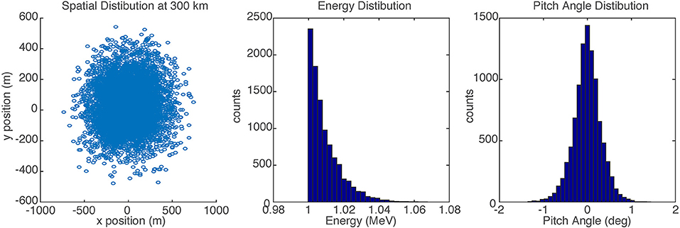
Figure 1. Input spatial, energy, and pitch angle distributions at 300 km altitude for the 1 MeV electron beam, based on simulations from Porazik et al. (2014).
Although ionization, optical, and X-ray signatures scale linearly with the beam energy (for the same electron energy), the choice of electron energy affects these signatures differently. Optical emissions and secondary ionization (leading to electron density disturbances) are nearly proportional to the total energy deposition, as described in section 3. However, X-ray emissions change considerably with electron energy, as the efficiency of bremsstrahlung production increases rapidly at higher energies. As a rule of thumb, approximately 0.2% of the beam energy is converted to X-rays for an electron energy of 1 MeV, while 2% is converted to X-rays for 5 MeV (Krause, 1998).
Ionization production is proportional to the beam energy; we use the rule-of-thumb from Rees (1963) that every 35 eV of energy deposited produces one electron-ion pair. This relationship was validated in Krause (1998). The ionization pair production is then used as a driving source in mesospheric chemistry models, including the Glukhov-Pasko-Inan (GPI) chemistry model (Glukhov et al., 1992; Lehtinen and Inan, 2009) and the Sodankylä Ion and Neutral Chemistry (SIC) model (Verronen et al., 2005; Turunen et al., 2009) to calculate electron density disturbances in the mesosphere and D-region ionosphere, along with the chemical response described in section 4. Here, the response is very strongly dependent on the electron energy. Due to higher electron-neutral collisions at lower altitudes, recombination rates are much higher, and so the electron density perturbation is suppressed. Because higher electron energies deposit energy at lower altitudes, they have a much weaker effect on the electron density disturbance for the same total energy.
In this section we revisit the ionization and optical signatures that were calculated in Marshall et al. (2014). Here, we use an electron energy of 1 MeV, and beam energies of 100 J or 1 kJ. These beams are actually divided into “pulses” every 5 ms and “subpulses” of 0.5 ms; however, most of the signatures we describe in this paper are not sensitive to the details of the pulse shape on times scales faster than 100 ms. Figure 2 shows the energy deposition profile for these two beams, along with the optical emission profiles for the 100 J beam. The ionization profile follows that of the energy deposition, under the approximation that every 35 eV deposited creates one electron-ion pair.
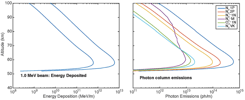
Figure 2. Left: Energy deposition profiles for 100 J and 1 kJ injections, integrated over the area and duration of the beam sequence. Right: Optical emission profiles for the 100 J injection. Both energy deposition and optical emissions scale linearly with the beam total energy.
We observe from Figure 2 that the energy deposition scales linearly with the beam energy. The optical emissions are dominated by N2 first positive (1P) and second positive (2P) emissions, both of which are spread over a large range of wavelengths; as such, detection above the background is much more difficult. The next highest intensity is the N first negative (1N) band system, which is heavily concentrated in two bandheads at 3,914 and 4,278 Å. Note that the N Meinel (M) band system has a relatively long lifetime (~6 μs) and a relatively high collisional quenching rate with N2, and so is quenched below ~90 km altitude where there is appreciable N2.
From our calculations of optical emissions, we can generate an energy partitioning that describes the fraction of the total injected energy that is emitted in each of a number of important lines and bands. The results, shown in Table 1, show the energy emitted as photons, after accounting for quenching and cascading. This partitioning is consistent with that of typical auroral emissions (Vallance Jones, 1974).
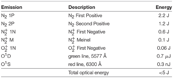
Table 1. Energy emitted in different optical bands from 100 J injected.
We focus on the N2 1P emissions, where we can zero-in on narrow emission lines (either 3,914 or 4,278 Å), reducing the background signal. We observe that about 2.2% of the total injected energy is converted to N2 1P emissions, and 0.6% is converted to 1N emissions. The atomic oxygen green and red line emissions are extremely weak, because the oxygen density is very low at 60 km altitude, and these emissions are rapidly quenched, with 0.7 and 110 s lifetimes.
Using this partitioning table, it is straightforward to make a back-of-the-envelope validation calculation of the expected signal seen by a detector on the ground. We consider an instrument designed to measure the 3,914 Å bandhead of the 1N system. A filter spanning 3,800–3,920 Å will capture 27% of the total 0.6 J emission; assuming a wavelength of 3900 Å, this fraction totals 3.2 × 10¹⁷ photons emitted in our band of interest. For simplicity we assume that all photons are emitted from 60 km altitude, and that they are emitted isotropically; and based on MODTRAN (Berk et al., 1987) simulations of the atmospheric transmission, we assume ~40% of the emission reaches the ground, while the rest is scattered or absorbed in the atmosphere. From these values we expect 1.7 × 10⁶ photons/m2 over the duration of the beam to reach the ground in our band of interest.
As an approximate instrument response, we consider an optical aperture of 50 mm diameter (a typical camera lens) with a field-of-view that is larger than the emitting region; then we can expect 3.3 × 10³ photons to be collected by the instrument. If the instrument is PMT-based, we can consider a window transmission efficiency of 90% and a PMT quantum efficiency (QE) of 28%. We consider instrument dark noise of 2 mA and background airglow of 2 Rayleighs per Ångstrom (R/Å) at 3,900 Å(Broadfoot and Kendall, 1968). With these noise sources together with shot noise, we calculate an expected signal-to-noise ratio in this PMT instrument of SNR ≃ 25 when sampled at 100 Hz.
Instead of a PMT-based system, we also consider measuring the beam spot with a wide field-of-view camera system. In this case, we start from the same 3.3 × 10³ photons to be collected by the instrument, assuming the same 50 mm diameter lens. The camera may have the same window transmission of 90%, but a higher QE of 60%, dark current of 0.0003 electrons/pixel/sec, and ~1 electron read noise. For such a system averaging frames to 5 fps, we expect an SNR ≃ 3.6, assuming the entire beam is contained in a single camera pixel. If instead the beam is spread over a few pixels, the SNR will be reduced from this value.
These calculations show that the optical signature from a 100 J beam should be detectable by either PMT or camera systems. The PMT system has the advantage of time resolution, valuable if the pulsing sequence is rapid and contains sub-pulses (but only if the subpulses maintain their separate during the beam propagation). The camera system has the advantage of simple spot detection in a sequence of images, as well as measurement of the spot location, invaluable for field-line tracing applications.
It is well-known that precipitation of relativistic electrons into the mesosphere can affect the chemistry of this region of the atmosphere. In particular, radiation belt precipitation leads to enhancement of odd nitrogen (NOx; Rusch et al., 1981) and odd hydrogen (HOx; Solomon et al., 1982), which ultimately affect ozone concentrations. In this section, we wish to investigate the possible chemical impact of our relativistic electron beam on the upper atmosphere.
The GPI model is a five-species model that includes electrons, heavy and light positive ions, and heavy and light negative ions; as such it cannot calculate the response of individual constituents of interest, such as NO, NO2, and so forth. Instead, we use the SIC model to calculate the response of these species. Described in detail in Verronen et al. (2016), SIC includes forcing from solar UV and soft X-rays, electron and proton precipitation, and galactic cosmic rays. The model solves for the densities of electrons and 70 ions, of which 41 are positive and 29 negative, and 34 neutral species, including O and O3; N, NO, NO2, NO3, and other species cumulatively referred to as NOx; and H, OH, HO2, and H2O2, cumulatively referred to as HOx.
In Figure 3, we compare these two models directly, using a 1 kJ beam injection over 100 pulses spaced every 5 ms. The two models use the same initial, background electron density, and then calculate the time response of the electron density profile. The two models compare favorably, though the SIC model predicts a 55% higher peak electron density, at an altitude 1 km lower than the GPI model. Considering the simplifications made in the GPI model to limit it to five species, this comparison shows that the GPI model provides a reasonably accurate estimate of the electron density response.
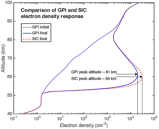
Figure 3. Electron density response of a 1,000 J beam injection over 0.5 s. The SIC model predicts a 50% larger peak electron density compared to the GPI model, with a peak response ~1 km lower in altitude.
Figure 4 shows the time-resolved electron density evolution along the beam axis for the 100 J (20 pulses in 100 ms) or 1 kJ (200 pulses in 1 s) beams, including the electron density profiles after each pulse. In both cases we observe that the electron density begins to saturate at the lower altitudes, due to the rapid recombination at these lower altitudes. After 20 pulses, the peak electron density of 3.9 × 109 cm−3 occurs at an altitude of 59 km. After 200 pulses, the peak electron density is 1.2 × 1010 cm−3 at 63 km altitude.
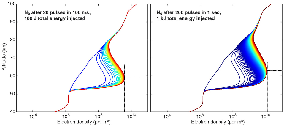
Figure 4. Electron density vs. altitude for a 100 J beam injection (left) and a 1 kJ beam injection (right). Blue to red colors show the electron density after each pulse. Dashed lines mark the peak density and altitude.
To determine the chemical response of the atmosphere, and in particular the NOx, HOx, and ozone signatures, we use the SIC model. Figure 5 shows the relative disturbances along the beam axis to each of these species after the 1 kJ injection over 0.5 s. The NOx density increases by only 0.5% from its background density, with a peak near 70 km altitude. The HOx density increases by about 0.4%, with the peak at 58 km. The ozone signature is negligible. Therefore, none of the beam applications under consideration should produce any deleterious side effects on the atmosphere.
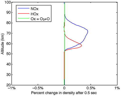
Figure 5. NOx, HOx, and Ox response following a 1 kJ injection over 0.5 s.
This small chemical response is encouraging, as it shows that this artificial beam injection will not have a significant, lasting effect on the atmosphere. Energetic electron precipitation is known to produce enhancements in NOx and HOx and the former can destroy ozone in the stratosphere. The ionization signature of our electron beam exceeds that of a typical radiation belt electron precipitation event; however, because the spatial extent is very small, but more importantly because the time duration of this precipitation is so short, the effect on atmospheric chemistry is negligible.
The chemical response shown in Figure 5 is for a single beam pulse, injecting 1 kJ of energy in 0.5 s. While the chemical response of this pulse is very small, it is possible that a sequence of pulses in the same region of the atmosphere could have a cumulative effect that is more pronounced. Seppälä et al. (2018) modeled the chemical response to a series of microbursts, with comparable time duration and density to our beam pulses, and showed a significant cumulative effect of enhanced NOx and HOx. However, their results considered a series of microbursts over a 6-h duration. Microbursts and microburst regions are also likely to cover a much larger spatial scale than our < 1 km electron beam (Blake and O'Brien, 2016; Crew et al., 2016); as such the beam experiment is unlikely to be able to produce a significant number of pulses in the same region of the atmosphere.
Some of the first work on artificial relativistic beam injection was conducted by Banks et al. (1987), Banks et al. (1990), Neubert and Banks (1992), and Neubert et al. (1996). Soon after, in the early 2000s, research into upper atmospheric discharges known as sprites was reaching maturity (e.g., Neubert et al., 2005; Inan et al., 2010). Neubert and Gilchrist (2004) went on to investigate the beam effects in the atmosphere, and suggested the possibility that the relativistic electron beam, upon its interaction with the atmosphere, could modify the conductivity enough to enhance the triggering of sprites at their typical triggering altitude of ~75 km (Stenbaek-Nielsen et al., 2010; Pasko et al., 2012). Here, we quantitatively assess that possibility using electrostatic field simulations.
We simulate the electron density disturbance in the upper atmosphere as described above and shown in Figure 4. This disturbance is three-dimensional in nature, based on the beam spreading calculated in the Monte Carlo model, and is approximately Gaussian with a radius of ~300 m. Next, we insert this electron density disturbance into the 2D, cylindrically-symmetric quasi-electrostatic (QES) field model of Kabirzadeh et al. (2015, 2017) and calculate the resulting electric fields. The model is quasi-electrostatic because it solves for dynamically-changing electric fields as time-changing driving sources (charge and current densities) are included.
By default, the QES model uses a uniform grid with either 500 or 1,000 m spatial resolution; however this resolution is clearly insufficient to resolve our 300 m radius disturbance. In order to avoid an excessively large simulation space, the model was modified to use a non-uniform grid; the horizontal resolution is ~70 cm at the beam axis, and smoothly increases non-linearly to the maximum grid size of ~350 m at a distance of 100 km. The grid is uniform with 250 m resolution in altitude, extending to a maximum altitude of 100 km.
The simulation uses the same background and perturbed ionosphere profile as in Figure 4. The electron-neutral collision frequency profile is determined using the method described by Marshall (2014). We wish to determine how the beam injection will change the electric field structure above a thunderstorm. To this end, we calculate the electric fields following the removal of 50 C of charge in a cloud-to-ground lightning discharge. Initially, a −50 C charge is placed at 5 km altitude, and a +50 C charge is placed at 10 km altitude. The uppermost charge is removed from the cloud (a 500 C-km charge moment change), causing the electrostatic fields to reconfigure.
The QES model solves for the time-resolved electric fields, but Figure 6 shows the fields after they have settled; the simulation does not account for charge reconfiguration in the cloud after the discharge. The top row shows the fields without a beam injection, while the bottom row shows the fields after the 1 kJ beam injection. The first two panels in each row show the horizontal (Er) and vertical (Ez) field components. The rightmost panel shows the reduced electric field E/Ek, i.e., the field magnitude normalized by the breakdown field, which scales with atmospheric pressure. For a sprite to initiate, we are looking for E/Ek ≥ 1, or log10(E/Ek) ≥ 0.
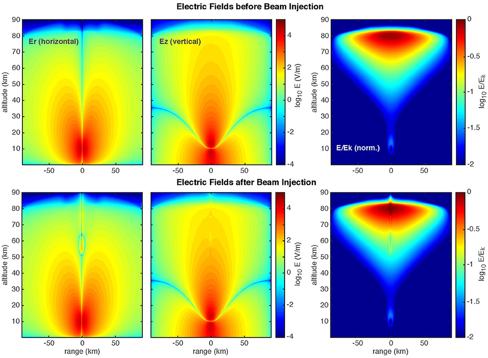
Figure 6. Electrostatic fields (top) before and (bottom) after beam injection. Rightmost panels show the normalized field E/Ek on a log10 scale.
Note that in this scenario, the beam is injected directly above the lightning discharge, where E/Ek is maximum, and that the beam is injected immediately following the lightning discharge, so that the beam modifies the post-discharge field configuration.
Figure 7 shows 1D slices of the reduced electric field (E/Ek) along the beam axis and at ranges from one to 50 km. These are the electric fields immediately after the discharge described above; these fields will recover back to the ambient fields in tens of seconds (e.g., Inan et al., 1996). Following the beam injection we observe significant variation in the field structure, especially on the beam axis at ~55 km and between 75 and 85 km. At 55 km the field is perturbed around the bottom of the electron density column. At the higher altitudes, as shown in the zoomed-in panel, we see that E>Ek within 1 km of the beam axis, while E < Ek before the beam injection. These results show that such an experiment could be made to increase the high-altitude electric fields and potentially trigger sprites, but only with very careful timing and fortuitous location.
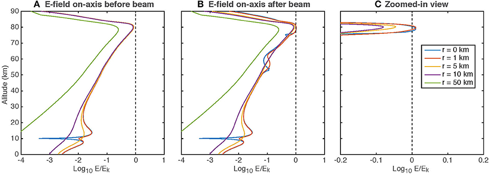
Figure 7. Normalized electric field log10(E/Ek) in 1D slices along the beam axis and at different radii. Left: Before the beam injection; middle: after beam injection; Right: zoomed-in view after beam injection.
These results provide an indication that the electron beam may be able to enhance the electrostatic field at sprite altitudes enough to trigger a discharge. However, we have not included the effect of the Earth's magnetic field, which at mid-latitudes, where lightning occurs, is strongly inclined. The magnetic field will push the ionization profile to slightly higher altitudes, and in turn affect this discharge triggering.
Similar to section 4 above, ionization production in pairs/m3/s are used as an input to chemistry models to determine the expected response of the mesosphere. We use both the SIC model described in section 4 as well as the GPI chemistry model. The latter is a four-species (Glukhov et al., 1992) or five-species (Lehtinen and Inan, 2009) simplified 1D model of mesospheric chemistry that considers electrons, light and heavy positive ions, and light and heavy negative ions. The set of ordinary differential equations relating the densities of these five species are presented in Lehtinen and Inan (2009). The modified electron density profile is used in this section to determine the expected radar and VLF scattering signatures, if any, that could be observed using these techniques.
Using our ionization profiles in section 3, we calculate the time-resolved electron density response in the mesosphere to determine the peak electron density expected as well as the recovery time of this signature. Figure 8 shows the resulting electron density disturbance and its evolution with time, for the 1 s duration of the pulse sequence (total energy of 1 kJ) and 1 s of its recovery. The background ionosphere density profile is calculated by the SIC model simulations; however the electron density disturbance is so large that the choice of background profile is not important. As in Marshall et al. (2014), the electron density disturbance recovers back to the background profile over timescales from tens of ms to many seconds, depending on altitude.
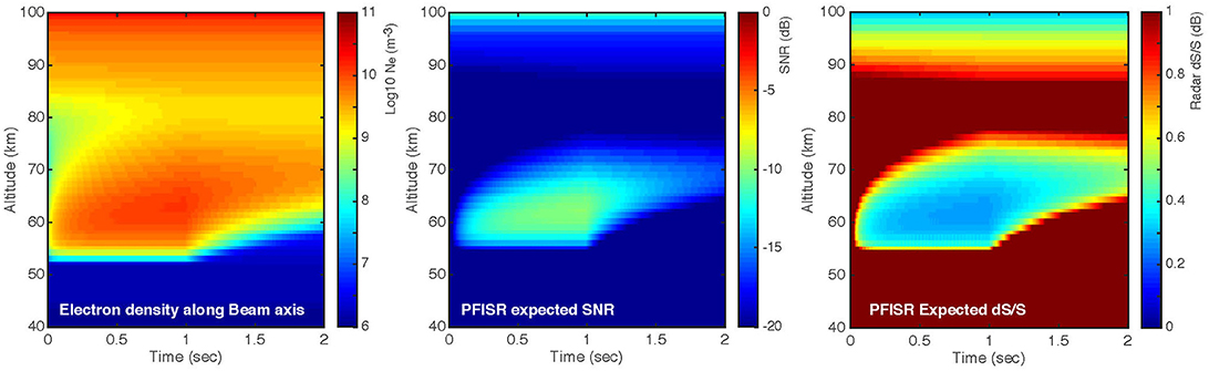
Figure 8. Left: Time-resolved electron density response for 1 s beam injection and 1 s recovery. Middle: expected SNR using PFISR radar parameters. Right: expected relative error, dS/S, again using PFISR radar parameters and pulse averaging as described in the text.
We consider the Poker Flat Incoherent Scatter Radar (PFISR) for our detectability estimate. We convert the electron density profile into an expected radar signal-to-noise ratio (SNR) using the relationship:
where ne is electron density, r0 = 100 km, r is range (or altitude if the radar beam is pointed toward the zenith), k = 4 π f/c is the Bragg wavenumber for the radar, is the electron Debye length in the plasma, and Tr = Te/Ti is the ratio of electron and ion temperatures. Thus the radar SNR is a function of the electron density and both the electron and ion temperatures. For our forward calculations of SNR, we assume Tr = 1 in the lower D-region, as electrons and ions are well-thermalized to the neutral temperature through the high collision frequency. At high electron density, kλD ≪ 1 and the equation simplifies to ; however the full relationship is required below ~80 km where kλD>1. The relationship in Equation (1) was derived for a PFISR experiment using 130 μs, 13-baud Barker codes; the expected SNR will change for different pulse lengths and radar performance.
A radar SNR < 1 does not mean the signal cannot be detected; by averaging pulses coherently and incoherently, we can dramatically improve the detectability, which is estimated as follows. We can combine N consecutive radar pulses using coherent averaging, up to the correlation time, which is about 200 ms at 65 km altitude. For a Lorentzian radar spectrum, the coherent processing gain is given by
where ω is the spectral width in Hz (about 5 Hz at 65 km altitude), and t is the inter-pulse period, taken to be 2 ms for this experiment. (Note that the radar “pulses” here, every 2 ms, are not the same as the beam “pulses” transmitted every 5 ms.) With N = 100 radar pulses in 200 ms, we calculated a coherent processing gain of G = 27. Finally, the relative error in the ISR power estimate is found by incoherently averaging K sets of coherent averages (e.g., Farley, 1969):
where K is the number of incoherent averages, in this case K = 5 to represent the five 200 ms periods. This relative error is plotted in the right panel of Figure 8. A relative error of dS/S = 1 indicates that the signal is 1σ above zero SNR; dS/S = 0.5 indicates 2σ above zero SNR; dS/S = 0.33 indicates 3σ above zero SNR, and so forth. We observe that the maximum SNR in these results is about −10 dB, corresponding to a minimum dS/S = 0.27. This shows that the electron beam pulse sequence of 1 kJ injected over 1 s should be marginally detectable by an incoherent scatter radar such as PFISR, when it is running Barker-type emission codes. Newer codes that increase the coherent gain combined with longer integration times will decrease dS/S and thus improve detectability. For example, a 50% increase in the averaging intervals would decrease dS/S to 0.22. Similarly, the electron beam signatures will likely be observable by the upcoming EISCAT 3D radar (Turunen, 2009).
Note that the radar signal is not sensitive to the background state of the ionosphere below 80 km; PFISR sees only noise below these altitudes under typical conditions, irrespective of the background D-region ionosphere state. The exception only occurs under very intense radiation belt precipitation, which can be detectable by PFISR below 70 km, and which may interfere with our beam detection.
Next, we consider whether or not the electron density disturbance from the beam would be observable through scattering of subionospheric very-low-frequency (VLF) transmitter signals. Powerful ground-based transmitters operated by the US Navy radiate VLF waves into the Earth-ionosphere waveguide, and the amplitude and phase of the signals observed by a distant receiver are particularly sensitive to the D-region ionosphere. At night, these waves reflect from altitudes ~80–85 km and are modified by electron density disturbances below the reflection height.
We test the possibility that the beam will perturb the VLF signal by simulating the propagation of VLF transmitter signals in the Earth-ionosphere waveguide, and comparing the amplitude and phase at a distant receiver before and after the beam pulse. We use the Finite-Difference Time Domain (FDTD) propagation model of Marshall (2012) and Marshall et al. (2017), which allows calculation of amplitude and phase for any frequency at any distance, and allows for small-scale ionospheric disturbances with ~500 m resolution or better.
The simulations shown here use a grid resolution of 500 m; as such, the electron density disturbance created by the beam only spans a few grid cells. We simulate a scenario shown in Figure 9, using the NLK transmitter. The pulse is injected above Poker Flat, AK, and a receiver is located 500 km further along the great-circle-path (GCP) connecting NLK and Poker Flat. To reduce the simulation time, we use a virtual transmitter 1,000 km away from Poker Flat instead of simulating the entire path. Figure 9 also shows the final electron density along the simulation path, with the beam injection shown at 1,000 km from the transmitter.
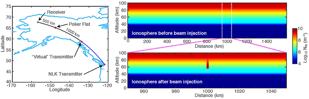
Figure 9. VLF scattering setup. To simulate the NLK transmitter we use a virtual transmitter 1,000 km from Poker Flat along the same great-circle-path. The receiver is 500 km past Poker Flat. Right: electron density profile along the path, showing the beam disturbance at 1000 km range from the transmitter.
To estimate the expected amplitude and phase perturbations to the VLF signal, we run two simulations: one without the beam-induced disturbance, and one with the disturbance. Figure 10 shows the amplitude and phase along the ground for both cases; the rightmost panels are zoomed-in views of the last 500 km. We see that the VLF signal is significantly perturbed, with up to 1 dB of amplitude change and ~10 degrees of phase change. For reference, in comparable VLF data, a minimum detectable perturbation is about 0.1 dB and 1 degree. Note that the ringing at the end of both simulations is a numerical artifact, due to the simulation being stopped before the highest-order modes have equilibrated.
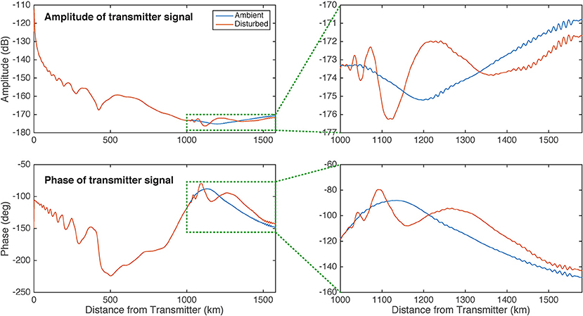
Figure 10. VLF amplitude and phase along the ground with and without the beam injection. A VLF receiver at 1,500 km would be expected to measure an amplitude change of ~1 dB and a phase change of ~10 degrees.
The natural variation in the D-region ionosphere will lead to variation in the received VLF signal amplitude and phase, as well as the received perturbation. The D-region variations can lead to amplitude variations at night of ~±5 dB, and phase variations of ~±50 degrees, varying on time scales of minutes to hours. A more comprehensive study, left to future work, is needed to assess the expected VLF perturbation under changing D-region conditions.
It is tempting to conclude that these results show that the subionospheric VLF method may be able to detect the beam-induced electron density disturbance, but we cannot yet make this conclusion. These simulations are 2D only, in range and altitude. As such, the disturbance imposed is effectively infinite in the third dimension; rather than a column of electron density, we have imposed a “wall” extending in and out of the page. This configuration is likely to produce a larger scattered signature than a single 300 m radius column. To better quantify the expected amplitude and phase perturbation, a full 3D simulation is needed. Such a simulation is extremely computationally expensive, and a single model to make this estimate does not currently exist. Nonetheless, these preliminary 2D simulations do not rule out the possibility that the subionospheric VLF method may be able to detect the beam-induced disturbance.
A relativistic beam of electrons injected from high altitudes has great potential for field line mapping, wave-particle interaction studies, and atmospheric studies (e.g., Delzanno et al., 2016), but most studies will require detection of the beam in the atmosphere. In this paper, we have provided results of simulations of the interaction of a beam of 1 MeV electrons with the upper atmosphere in order to assess its detectability via numerous diagnostic techniques. We have further explored the effects of the electron beam on the atmosphere, in terms of the chemical and electrodynamic response of the region. For the latter, we show that the beam injection into the atmosphere may aid in the triggering of sprites at high-altitude, though the inclination of the Earth's magnetic field must be taken into account.
We simulate a beam of 1 MeV electrons totaling 100 J or 1 kJ of energy. Monte Carlo simulations provide an estimate of the ionization produced by these beams and the altitude distribution and horizontal distribution of this ionization. Optical emissions are then calculated from the ionization production, and we determine the photon production taking into account quenching and cascading in a suite of N2, , and O emission band systems. We estimate the expected signal-to-noise ratios in a photomultiplier tube (PMT)-based detection system, and in an all-sky camera. These two systems have different advantages. The PMT system has the speed (1 kHz) necessary to detect individual sub-pulses in the beam pattern, but does not have any spatial information; the all-sky camera system lacks time resolution but can locate the beam spot in the sky with high accuracy, a critical requirement for many of the science applications of the electron beam.
Both systems should have sufficiently high SNR to detect the spot in the upper atmosphere. However the SNR values calculated in section 3 depend on a number of parameters which will vary for different systems. In particular, the PMT system depends on the choice of PMT and its wavelength response, noise characteristics, and the instrument sampling rate, in addition to optical design parameters. The camera system similarly depends on parameters of the camera chosen and the optical system, including filter transmission and passband. As such, the expected SNR will vary for different systems, and the system must be carefully designed to be optimized for the expected signatures. However, our calculations of the SNR and detectability are validated by the SEPAC experiments (Neubert et al., 1995) who observed optical emissions of 1–5 kR with a factor of 7.5 higher energy flux than our proposed experiments.
Similarly, the radar signatures presented in section 6.1 must be considered for a particular experiment design. The SNR calculated by Equation (1) will change for different radar pulse parameters and for different ISRs. What's more, the detectability in ISR appears to be marginal with standard radar beam pulse codes. New beam schemes and longer integration times will be required to ensure detectability.
One important characteristic of ISRs that must not be overlooked is that these instruments can provide detection of the electron beam in dayside conditions, where optical detection methods are not possible. An entire class of magnetospheric phenomena, such as plasma entry through the dayside boundary layer between the solar wind and the magnetosphere, still have several fundamental outstanding questions that can be answered with the appropriate match between magnetospheric in-situ measurements and the unambiguous identification of the ionospheric foot-point.
Subionospheric remote sensing has its own set of difficulties for detection. The receiver needs to be downstream of the ionization patch relative to the transmitter, although some deviation is likely acceptable; the forward scattering of the ~300 m radius patch will have some angular distribution. However, it is unclear at this point how strong the scattering will be in a full, three-dimensional scattering scenario. We require a full 3D scattering model to fully assess the VLF scattering. However, such a 3D model will be computationally expensive, since it requires ~100 m resolution around the ionization patch, but a transmission distance of thousands of kilometers.
In summary, in this paper we have presented a range of signatures of the 1 MeV beam interaction with the upper atmosphere, and quantified the expected signatures in different diagnostics. Optical detection of the beam spot remains the most promising method, and a combination of PMT and camera detection would allow both time resolution and spatial location of the spot. Radar and VLF detection of the ionization patch are likely marginal, though the latter requires further study.
The simulation outputs used in the analysis and results herein are available for download from Github at https://github.com/ram80unit/FrontiersBeamPaper.
RM conducted GPI chemistry simulations and VLF propagation simulations, analyzed simulation outputs, created figures, and wrote the manuscript text. WX conducted Monte Carlo simulations of electron precipitation in the atmosphere. AK conducted SIC model simulations of the atmospheric response. RK developed the 3D QES model and conducted simulations using that model. ES is the project PI and contributed to the analysis of radar signatures.
This work was supported by NSF INSPIRE award 1344303 and NSF MAG award 1732359. AK was supported by the Tenure Track Project in Radio Science at Sodankylä Geophysical Observatory.
RK was employed by company Zoox, Inc. The remaining authors declare that the research was conducted in the absence of any commercial or financial relationships that could be construed as a potential conflict of interest.
We thank Dr. Roger Varney for invaluable help in assessing the radar signatures of the beam. The authors thank Drs. Joe Borovsky, Geoff Reeves, and Gian Luca Delzanno for valuable discussions and their tireless pursuit of the CONNEX mission. We also thank Dr. Esa Turunen for his contributions with the SIC model.
Banks, P. M., Fraser-Smith, A. C., and Gilchrist, B. E. (1990). “Ionospheric modification using relativistic electron beams,” in AGARD Conference Proceedings (Stanford, CA).
Banks, P. M., Fraser-Smith, A. C., Gilchrist, B. E., Harker, K. J., Storey, L. R. O., and Williamson, P. R. (1987). New Concepts in Ionospheric Modification. Final Report AFGL-TR-88-0133, Stanford University.
Berk, A., Bernstein, L. S., and Robertson, D. C. (1987). MODTRAN: A Moderate Resolution Model for LOWTRAN. Technical report. Spectral Sciences Inc., Burlington, MA.
Blake, J., and O'Brien, T. (2016). Observations of small-scale latitudinal structure in energetic electron precipitation. J. Geophys. Res. Space Phys. 121, 3031–3035. doi: 10.1002/2015JA021815
Broadfoot, A. L., and Kendall, K. R. (1968). The airglow spectrum, 3100–10,000a. J. Geophys. Res. 73, 426–428.
Burch, J. L., Mende, S. B., Kawashima, N., Roberts, W. T., Taylor, W. W. L., Neubert, T., et al. (1993). Artificial auroras in the upper atmosphere 1. electron beam injections. Geophys. Res. Lett. 20, 491–494.
Crew, A. B., Spence, H. E., Blake, J. B., Klumpar, D. M., Larsen, B. A., O'Brien, T. P., et al. (2016). First multipoint in situ observations of electron microbursts: Initial results from the NSF firebird II mission. J. Geophys. Res. Space Phys. 121, 5272–5283. doi: 10.1002/2016JA022485
Delzanno, G. L., Borovsky, J. E., Thomsen, M. F., Gilchrist, B. E., and Sanchez, E. (2016). Can an electron gun solve the outstanding problem of magnetosphere-ionosphere connectivity? J. Geophys. Res. Space Phys. 121, 6769–6773. doi: 10.1002/2016JA022728
Dors, E. E., MacDonald, E. A., Kepko, E. L., Borovsky, J. E., Reeves, G. D., Delzanno, G. L., et al. (2017). CONNEX: Concept to Connect Magnetospheric Physical Processes to Ionospheric Phenomena. Technical report. Los Alamos National Lab (LANL), Los Alamos, NM.
Farley, D. (1969). Incoherent scatter power measurements; a comparison of various techniques. Radio Sci. 4, 139–142.
Glukhov, V. S., Pasko, V. P., and Inan, U. S. (1992). Relaxation of transient lower ionospheric disturbances caused by lightning-whister-induced electron precipitation bursts. J. Geophys. Res. 97, 16971–16979.
Inan, U. S., Cummer, S. A., and Marshall, R. A. (2010). A survey of ELF and VLF research on lightning-ionosphere interactions and causative discharges. J. Geophys Res. 115, A00E36. doi: 10.1029/2009JA014775
Inan, U. S., Pasko, V. P., and Bell, T. F. (1996). Sustained heating of the ionosphere above thunderstorms as evidenced in “early/fast” VLF events. Geophys. Res. Lett. 23, 1067–1070.
Kabirzadeh, R., Lehtinen, N., and Inan, U. S. (2015). Latitudinal dependence of static mesospheric e-fields above thunderstorms. Geophys. Res. Lett. 42, 4208–4215. doi: 10.1002/2015GL064042
Kabirzadeh, R., Marshall, R. A., and Inan, U. S. (2017). Early/fast VLF events produced by the quiescent heating of the lower ionosphere by thunderstorms. J. Geophys. Res. Atmospheres 122, 6217–6230. doi: 10.1002/2017JD026528
Krause, L. H. (1998). The Interaction of Relativistic Electron Beams with the Near-Earth Space Environment. Ph.D. thesis, University of Michigan.
Lehtinen, N. G., and Inan, U. S. (2009). Full-wave modeling of transionospheric propagation of VLF waves. Geophys. Res. Lett. 36:L03104. doi: 10.1029/2008GL036535
Marshall, R. A. (2012). An improved model of the lightning electromagnetic field interaction with the D-region ionosphere. J. Geophys. Res. 117:A3. doi: 10.1029/2011JA017408
Marshall, R. A. (2014). Effect of self-absorption on attenuation of lightning and transmitter signals in the lower ionosphere. J. Geophys. Res. Space Physics, 119, 4062–4076. doi: 10.1002/2014JA019921
Marshall, R. A., Nicolls, M. J., Sanchez, E., Lehtinen, N. G., and Neilson, J. (2014). Diagnostics of an artifical relativistic electron beam interacting with the atmosphere. J. Geophys. Res. 119, 8560–8577. doi: 10.1002/2014JA020427
Marshall, R. A., Wallace, T., and Turbe, M. (2017). Finite-difference modeling of very-low-frequency propagation in the earth-ionosphere waveguide. IEEE Trans. Ant. Prop. 65, 7185–7197. doi: 10.1109/TAP.2017.2758392
Neubert, T., Allin, T. H., Blanc, E., Farges, T., Haldoupis, C., Mika, A., et al. (2005). Co-ordinated observations of transient luminous events during the EuroSprite2003 campaign. J. Atmos. Solar Terr. Phys. 67, 807–820. doi: 10.1016/j.jastp.2005.02.004
Neubert, T., and Banks, P. M. (1992). Recent results from studies of electron beam phenomena in space plasmas. Planet. Space Sci. 40, 153–183.
Neubert, T., Burch, J. L., and Mende, S. B. (1995). The SEPAC artificial aurora. Geophys. Res. Lett. 22, 2469–2472,
Neubert, T., Gilchrist, B., Wilderman, S., Habash, L., and Wang, H. J. (1996). Relativistic electron beam propagation in the earth's atmosphere: modeling results. Geophys. Res. Lett. 23, 1009–1012.
Neubert, T., and Gilchrist, B. E. (2002). Particle simulations of relativistic electron beam injection from spacecraft. J. Geophys. Res. 107:1167. doi: 10.1029/2001JA900102
Neubert, T., and Gilchrist, B. E. (2004). Relativistic electron beam injection from spacecraft: performance and applications. Adv. Space Res. 34, 2409–2412. doi: 10.1016/j.asr.2003.08.081
Neupert, W. M., Banks, P. M., Brueckner, G. E., Chipman, E. G., Cowles, J., McDonnell, J. A. M., et al. (1982). Science on the space shuttle. Nature 296, 193–197.
Pasko, V. P., Yair, Y., and Kuo, C.-L. (2012). Lightning related transient luminous events at high altitude in the earth's atmosphere: Phenomenology, mechanisms and effects. Space Sci. Rev. 168, 475–516. doi: 10.1007/s11214-011-9813-9
Porazik, P., Johnson, J. R., Kaganovich, I., and Sanchez, E. (2014). Modification of the loss cone for energetic particles. Geophys. Res. Lett. 41, 8107–8113. doi: 10.1002/2014GL061869
Rees, M. H. (1963). Auroral ionization and excitation by incident energetic electrons. Planet. Space Sci. 11, 1209–1218.
Rusch, D., Gérard, J.-C., Solomon, S., Crutzen, P., and Reid, G. (1981). The effect of particle precipitation events on the neutral and ion chemistry of the middle atmosphere–I. odd nitrogen. Planet. Space Sci. 29, 767–774. doi: 10.1016/0032-0633(81)90048-9
Seppälä, A., Douma, E., Rodger, C., Verronen, P., Clilverd, M. A., and Bortnik, J. (2018). Relativistic electron microburst events: modeling the atmospheric impact. Geophys. Res. Lett. 45, 1141–1147. doi: 10.1002/2017GL075949
Solomon, S., Reid, G. C., Roble, R. G., and Crutzen, P. J. (1982). Photochemical coupling between the thermosphere and the lower atmosphere: 2. D region ion chemistry and the winter anomaly. J. Geophys. Res. 87, 7221–7227.
Stenbaek-Nielsen, H. C., Haaland, R., McHarg, M. G., Hensley, B. A., and Kanmae, T. (2010). Sprite initiation altitude measured by triangulation. J. Geophys. Res. 115:A00E12. doi: 10.1029/2009JA014543
Stone, N. H. and Bonifazi, C. (1998). The TSS-1R mission: Overview and scientific context. Geophys. Res. Lett. 25, 409–412
Turunen, E. (2009). “Eiscat 3d-the next generation european incoherent scatter radar system,” in EGU General Assembly Conference Abstracts (Vienna), 11032.
Turunen, E., Verronen, P. T., Seppälä, A., Rodger, C. J., Clilverd, M. A., Tamminen, J., et al. (2009). Impact of different energies of precipitating particles on nox generation in the middle and upper atmosphere during geomagnetic storms. J. Atmos. Solar Terres. Phys. 71, 1176–1189. doi: 10.1016/j.jastp.2008.07.005
Verronen, P. T., Andersson, M. E., Marsh, D. R., Kovacs, T., and Plane, J. M. C. (2016). WACCM-D—whole atmosphere community climate model with d-region ion chemistry. J. Adv. Modeling Earth Sys. 8, 945–975. doi: 10.1002/2015MS000592
Verronen, P. T., Seppälä, A., Clilverd, M. A., Rodger, C. J., Kyrölä, E., Enell, C.-F., et al. (2005). Diurnal variation of ozone depletion during the October–November 2003 solar proton events. J. Geophys. Res. 110:A09S32. doi: 10.1029/2004JA010932
Keywords: radiation belts, atmosphere, electron beam, chemistry, sprites, subionospheric VLF
Citation: Marshall RA, Xu W, Kero A, Kabirzadeh R and Sanchez E (2019) Atmospheric Effects of a Relativistic Electron Beam Injected From Above: Chemistry, Electrodynamics, and Radio Scattering. Front. Astron. Space Sci. 6:6. doi: 10.3389/fspas.2019.00006
Received: 30 October 2018; Accepted: 29 January 2019;
Published: 19 February 2019.
Edited by:
Joseph Eric Borovsky, Space Science Institute, United StatesReviewed by:
Torsten Neubert, Technical University of Denmark, DenmarkCopyright © 2019 Marshall, Xu, Kero, Kabirzadeh and Sanchez. This is an open-access article distributed under the terms of the Creative Commons Attribution License (CC BY). The use, distribution or reproduction in other forums is permitted, provided the original author(s) and the copyright owner(s) are credited and that the original publication in this journal is cited, in accordance with accepted academic practice. No use, distribution or reproduction is permitted which does not comply with these terms.
*Correspondence: Robert A. Marshall, cm9iZXJ0Lm1hcnNoYWxsQGNvbG9yYWRvLmVkdQ==
Disclaimer: All claims expressed in this article are solely those of the authors and do not necessarily represent those of their affiliated organizations, or those of the publisher, the editors and the reviewers. Any product that may be evaluated in this article or claim that may be made by its manufacturer is not guaranteed or endorsed by the publisher.
Research integrity at Frontiers
Learn more about the work of our research integrity team to safeguard the quality of each article we publish.