 Utku Boz
 Raman Goyal
 Robert E. Skelton2*
95% of researchers rate our articles as excellent or good
Learn more about the work of our research integrity team to safeguard the quality of each article we publish.
Find out more
ORIGINAL RESEARCH article
Front. Astron. Space Sci. , 13 December 2018
Sec. Space Robotics
Volume 5 - 2018 | https://doi.org/10.3389/fspas.2018.00041
This article is part of the Research Topic Imagining the Future of Astronomy and Space Science View all 10 articles
Tensegrity offers lightweight deployable structures for use in many engineering disciplines. Among all of the available tensegrity forms, D-Bar has a potential for combined applications of sensing, actuation, and structural support. In this paper, we enhance the minimal mass formulation of the D-Bar by including yielding of the compressive members as a design constraint in contrast to the previous assumption which considers buckling as the sole failure mechanism. In addition, we analyze the length and force gains of a D-bar system analytically by considering the minimal mass D-bar as the design constraint. Furthermore, we calculate the stiffness of the D-Bar and when appropriate use as design constraints as well. To enhance the minimal mass properties of the D-Bar, we combine T-bar and D-bar systems. The analysis shows that these structures are the basis for effective force transducers, force-controlled actuators, and efficient deployable compressive structures.
We consider tensegrity as any network of axially-loaded prestressable members (Skelton and de Oliveira, 2009). Tensegrity structures are proven to be minimum mass for various loading conditions (Skelton and de Oliveira, 2009). It is important to minimize the mass of structure for space applications. Therefore, tensegrity can be used to provide solutions to many structural problems in space, such as artificial gravity space habitats (Skelton and Longman, 2014; Goyal et al., 2017), minimum mass structures for space (Skelton and de Oliveira, 2010; Nagase and Skelton, 2014), and impact lander for planetary explorations (SunSpiral et al., 2013; Rimoli, 2016).
Tensegrity structures offer various functions such as load-bearing, sensing, actuation, and morphing capabilities (Skelton and de Oliveira, 2009). Moreover, by selecting different material for each member of the network or using various combinations of materials, it is possible to create structures with special electrical, acoustic or mechanical properties. Early tensegrity contributors include (Snelson, 1965; Fuller et al., 1975; Pugh, 1976; Calladine, 1978; Pellegrino, 1986; Murakami and Nishimura, 2001; Sultan and Skelton, 2004; Motro, 2011). Efficient models for tensegrity dynamics are proposed in Skelton (2005) and Goyal and Skelton (2018) representing the dynamics of tensegrity structures with a new matrix form and shape-changing control strategies.
Beyond minimal mass properties, there are studies showing the suitability of tensegrity structures for sensing and actuation. Sultan and Skelton used an icosahedron tensegrity structure to develop a 6 d.o.f sensor structure (Sultan and Skelton, 2004). They employed tendons of the tensegrity structure as sensing members and showed that the tensegrity structure is capable of measuring the forces and torques in all directions. Furthermore, they proved that a tensegrity structure offers fault-tolerant, redundant architecture for more precise measurement of the environmental loading conditions. Hagiwara and Oda (2010) used the tendons of the tensegrity prism as actuators to transform a structure between different configurations. They numerically and experimentally evaluated the capabilities of a tensegrity prism for form-finding applications and showed its promising structural concept for robotic applications. A recent study by Koizumi et al. (2012) demonstrates a tensegrity robot that is driven by soft actuators. They employed pneumatic actuators to experimentally demonstrate the capability of the tensegrity mechanism to perform the requested motion path on a flat surface.
The D-bar tensegrity topology introduced in Skelton and de Oliveira (2009) is investigated here further for its use in sensing and actuating functions. First, the minimal mass design for the D-Bar is extended to include the yielding as a possible failure mechanism as the number of complexity is increased. Then, using the minimal mass configuration, an analytical framework is developed to utilize the D-Bar as a sensor or actuator for either length or force under compressive configuration using structural parameter relations. Later, as an essential element to any sensor or actuator, formulation to evaluate the stiffness of the structure is derived for compressive performance. Finally, a novel structure configuration combining T-Bar and D-Bar is proposed and a brief overview of its minimal mass properties and parametric relations as well as its stiffness properties are presented. For each step of derivation, detailed examples are provided to illustrate the potential use of the proposed structural paradigm based on tensegrity D-Bar.
The paper is organized as follows. Section 2 describes the D-Bar, the concept of self-similarity, and reviews the minimal mass properties of the tensegrity D-Bar under buckling constraints. sections 3 derives the analytical relations between structural parameters of D-bar as sensors and actuators for planar and 3D D-Bar networks. Section 4 presents the stiffness formulation for the planar and 3D D-Bar and section 5 determines the minimum mass to satisfy a given stiffness requirement in the planar configuration. Section 6 describes the novel configuration combining the planar T-Bar and D-Bar. Section 7 gives an example to design minimal mass loaded platform to deploy to a specified shape. Finally, section 8 provides some conclusions.
Figure 1 illustrates a D-bar structure of complexity 1. There are 4 compressive members (bars) and 1 tensile member (string) in the structure, where L is the length of the D-Bar, lb is the bar length and s is the string length. It has been shown Skelton and de Oliveira (2009) that, for complexity q = 1, and any given applied force F, the normalized mass ratio (μ) under buckling constraints is given by:
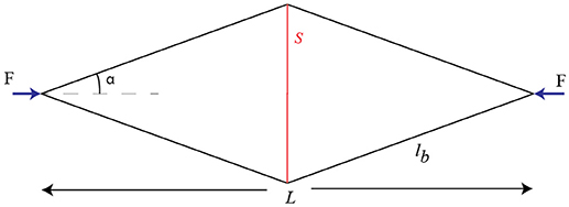
Figure 1. Configuration of the planar D-bar (Complexity q = 1).
where μ is the ratio of the mass of the D-bar system and the minimal mass of a solid bar that could take the same external load. The term ϵ includes the material properties, the magnitude of the compressive force, and overall length of the structure and is defined as:
where ρs and ρb are mass densities of the string and bar materials, respectively. Eb is the elastic modulus of the bar material, σs is the yield stress of the string material and L is the length of the D-Bar. When μ < 1, the D-bar system has less mass than a single bar that could take the same load. The necessary condition for mass ratio to be less than 1 is or equivalently α < 29.477°. Therefore, for μ < 1, one can replace any bar in a structure with this D-bar, where, each bar is replaced with yet another D-bar. This procedure is called self-similar iteration. A structure obtained after q self-similar iterations is called a D-bar system of complexity q.
Figure 2 shows a D-bar system of complexity q = 2, where a different α is used for 2nd iteration. The strings of the D-Bar fail due to yielding, but the bars may fail due to either yielding or buckling. For a complexity q planar D-bar, with different choices for α at each self-similar iteration, the normalized mass at the buckling constraint is given in Skelton and de Oliveira (2009) as:
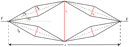
Figure 2. Planar D-Bar (Complexity q = 2. tq and sq are the tension and the length of the strings at level q. lb represents bar length).
Figure 3 shows a special case of the D-Bar structures where angles are equal on each complexity level (∀αi = α). Note that to ensure the same angle for each self-similar iteration during the application, the duplicate members can be combined into a single member.
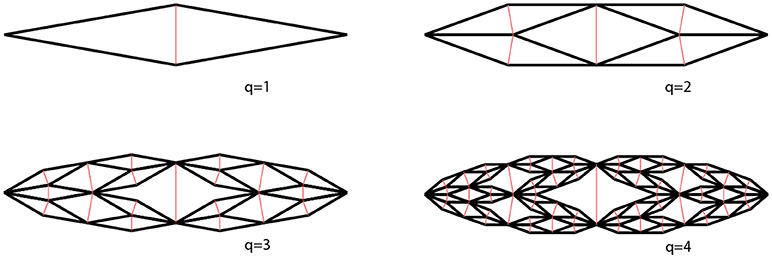
Figure 3. Configurations of the planar D-Bar Self-Similar structure with constant α = 10°.
When the same angle α is used for self-similarity, the normalized mass from Equation (3) for any complexity q reduces to:
For the three dimensional (3D) D-Bar shown in Figure 4, for the special case ∀αi = α, Equation (4) is modified as follows:
where subscript is used to represent the 3D configuration. The term N appearing in Equation (5) stands for maximum number of bars connected to the same point when q = 1. For example, N = 3 for the D-Bar configuration shown in Figure 4.
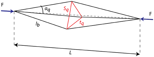
Figure 4. 3D D-Bar Under Compressive Load F (Complexity q = 1).
As previously stated, the mode of failure in the bars can be yielding or buckling depending on the configuration or the force applied. For any D-Bar system of complexity q, yielding becomes the mode of failure if the following inequality is satisfied as shown in the Skelton and de Oliveira (2009):
For the 3D D-Bar, following the same procedure for the derivation of Equation (6) as described in Skelton and de Oliveira (2009) the same condition changes to:
Clearly, these equations show that yielding becomes the mode of failure if complexity q is large enough.
Example 1: Consider the material properties given in Table 1 for bars and strings (Aluminum for bars and Ultra High Molecular Weight Polyethylene (UHMWPE) for strings). Figures 5A,B show the limit values of for planar and 3D D-Bars, respectively, by considering 3 different angular configurations α = 10°, 15° and 20°. The shaded region indicates the area satisfying the inequalities (6) and (7). The primary mode of failure changes from buckling to yielding when the is greater than value of the line specific to each angular configuration.

Table 1. Material properties.
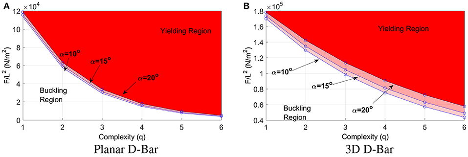
Figure 5. Buckling and yielding regions with α = 10°, 15°, and 20°. The ordinate shows and the abscissa shows complexity q. (A) Planar D-Bar. (B) 3D D-Bar.
Planar D-Bar changes its primary mode of failure for lower values of than the 3D D-Bar. On the other hand, the higher the angle, the higher the value of before the mode of failure changes from buckling to yielding.
This section provides the relationship between the structural parameters of the D-Bar. For the remainder of the paper, it is assumed that bars are rigid, strings are elastic, and the mass of the joints is negligible. Figures 2, 4 shows the general form of the D-bar under compressive loading.
The length of the D-Bar is specified by the configuration of its structural members. Given that the overall length L of the D-Bar changes with the compression, it is possible to quantify the overall length change by tracking the length change over the strings of the D-Bar. The strings of the D-Bar undergo the same length change in the same complexity level. Since there are more than one strings when the complexity level is bigger than 1, it is possible to measure the same quantity using multiple structural members.This property of the D-Bar makes it suitable displacement sensor with many equivalent outputs. Therefore, the sensor configuration is robust because it is possible to measure the displacement even when one or more sensor structural members fail. Furthermore, the versatility of the D-Bar ensures the actuation performance governed by exactly the same relations for displacement.
Theorem 1: The Gain G1(q), defined as the ratio of change in length of the D-bar to change in length of the shortest string at complexity q, is given by:
where , , αi0 is the initial angle at complexity level i and αi is the final angle at complexity level i after the D-Bar is statically balanced. The extension of the same relation to the 3D D-Bar, is given as:
where the superscript 3D indicates that the relations are derived for the three dimensional case.
Proof: Recalling the rigid bar assumption, we can formulate the geometrical relations between the bar length lb, initial length of the D-bar L0, final length of the D-bar L and angles αi, αi0 as:
which leads to . The change in the length of the D-Bar can be written as:
The relation between ΔSq and lb can be written as:
Substituting from Equations (11) and (12) into , we get back Equation (8). The same approach is followed to get Equation (9) for the geometrical relations of the 3D D-Bar.□
Example 2: Consider a D-bar structure where ∀αi = α, substituting α to αi in Equation (8), we get:
where h = α−α0. Taking the limit as h approaches zero, Equation (13) yields:
Similarly, for N = 3, can be written as:
Note that the − sign in Equations (14) and (15) suggests that if length of the D-bar reduces, length of the string at complexity level q increases. Figure 6 shows the magnitude of the gain G1(q) and for various angle and complexity configurations. The angle α is evaluated for the values of 5°, 10°, and 15°. From Figure 6, it is clear that the increasing complexity and increasing angle lead to higher ratios of ΔL and ΔSq. To summarize, if the structure is employed for length related parametric modifications, the angle and complexity should be selected as high as possible to relate the higher level of displacements to a smaller amount of length change for the strings at level q. This observation is valid for both planar and 3D versions with values of the being greater than the G1(q).
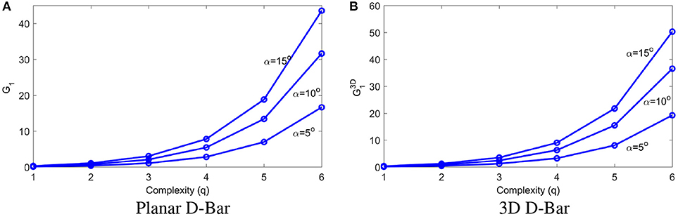
Figure 6. Gains G1(Equation 14) and (Equation 15) for complexity q and angle α combinations. (A) Planar D-Bar. (B) 3D D-Bar.
By tracking the tension over the strings of the D-Bar at higher complexities, it is possible to estimate the compressive force F. Therefore, it is possible to create a configuration with inherent force sensing properties. Furthermore, similar to the configuration for length gain, the sensing capability is robust to the structural failures within the D-Bar itself due to the presence of multiple members with the same contribution to the load-bearing configuration. In other words, the presence of multiple strings leads to a successful force sensor even when one or more strings malfunction. In addition, similar to the length gain, it is also possible to use the D-Bar as actuator governed by the same relations observed for the sensor.
Theorem 2: The Gain G2(q), defined as the ratio of the external force applied to the tension in the shortest string at complexity q level, is given by:
Extension of the planar relation to the 3D yields:
Proof: We can write the equation of static balance by looking at the node in Figure 7 as:
where fb is force on the bar. The bar force is related to the compressive force F as:
Combining Equations (18) and (19), Equation (16) is found. Adopting the same method, it is straightforward to derive the relation given in Equation (17).□
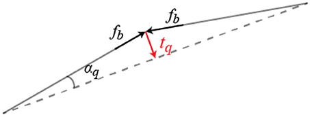
Figure 7. The bar-string connection at complexity level q.
Example 3: In this example consider the special case of the D-Bar for both planar and 3D versions introduced in example 2. Substituting α to αi in Equation (16) leads to the gain relation as:
For 3D configuration, the gain becomes:
Figure 8 shows the relation between the F and the tq for both planar and 3D versions. From Figure 8, it is concluded that the value of the G2(q) increases with the increasing number of complexity q and decreases with the increasing angle of the D-bar angle α. It is also worth stating that the gains G1(q) and G2(q) show opposite behavior with respect to the D-bar angle α.
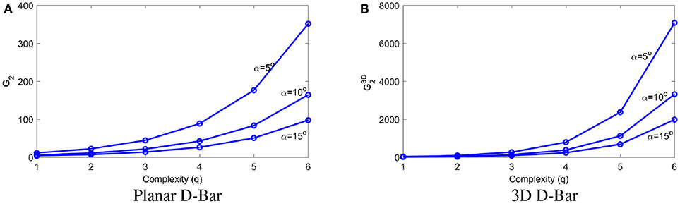
Figure 8. Gains G2(q) (Equation 20) and (Equation 21) for complexity q and angle α combinations. (A) Planar D-Bar. (B) 3D D-Bar.
Using the Hooke's law and the length changes over the strings of the D-Bar at higher complexities, it is possible to estimate the compressive force F. Therefore, it is possible to track the force change using the length changes over the strings of the sensor. Similar to the configuration for length gain and force gain, the sensor configuration is also robust to the structural failures.
Lemma 1: Let the extensional stiffness kq be given. The Force to Length Gain G3(q), defined as the ratio of the applied force to the change in length of the shortest string in a D-bar system of complexity q, is given by:
The extension of the expression given in Equation (22) yields:
Proof: Using the assumption 2 and replacing the tq with the expression tq = kqΔSq in Equation (16), it is straightforward to see the relation in Equation (22). The gain G3(q) is related to the gain G2(q) by the linear relationship G3(q) = kqG2(q). The relations between the and are exactly the same as explained for the planar configuration.
Example 4: This example presents a minimal mass sensor design. Consider the minimal mass formulation of the planar and 3D versions of D-Bar when ∀αi = α as given in Equations (4) and (6) where i denotes the each self-similar iteration such that i = 1q. The materials are selected as given in Table 1. Given the data: L = 0.25m, α = 10°, F = 1000N, we find ϵ = 0.0039. The normalized mass of the structure vs. complexity q is shown in Figure 9.
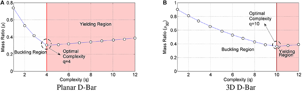
Figure 9. Mass ratio (Equation 4) and Mass ratio (Equation 5) for parameters given in Example 4. (A) Planar D-Bar. (B) 3D D-Bar.
Using the relation shown in Equation (6), it is possible to find the complexity at which yielding becomes the mode of failure. In this example, if the complexity q is greater than 3 for the planar configuration, yielding becomes the mode of failure. On the other hand, for the 3D configuration, the mode of failure becomes yielding when q is greater than 9. Such a difference is due to the fact that the 3D D-bar shares the compressive load with more members. In order to find the optimal complexity of the D-bar for the minimal mass configuration, the bar masses should be incorporated for yielding conditions after the corresponding complexity levels. The mass ratios given in Equations (4) and (5) are no longer valid if the yielding is the mode of failure. The modified versions of the μ and for yielding are given by:
where τ is similar to ϵ and is given by:
where σb is the yield stress of the bar material.
Figures 9A,B show the normalized mass of the planar and 3D configurations. Optimal complexity in terms of minimal mass is achieved when q = 4 for the planar D-Bar and q = 10 for the 3D D-Bar. For those complexities normalized mass ratios μ and μ3D become 0.30 and 0.36, corresponding to a mass savings of 70% and 64%, respectively. For the selected α and the complexities of the two configurations the gain G1(q) becomes G1(4) = −5. Evaluation of the G2(q) yields the value of G2(4) = 43. If the gains for the 3D version are evaluated the resultant value of the gains become and . For G3(q) we need to have the string stiffness kq at the complexity level q. The length of the string at the complexity level i for a planar D-Bar is given by:
The stiffness of the string on complexity level i can be calculated as:
where Es is the elastic modulus of the strings at complexity level i, and Ai is the cross sectional area of the string. Substituting for and leads to:
Equation (28) indicates that the minimal mass planar D-Bar has the same string stiffness for every complexity level i. Then, the G3(q) can be written as:
Now for the evaluation of the gain , the string stiffness for the complexity q must be known. The string stiffness of the 3D D-Bar when , and the string length for any complexity q becomes:
Recalling the relation and replacing the as:
the cross sectional area of the string becomes:
Combining all of those expressions give the stiffness of a string at the complexity level i as:
Using the definition of the and N = 3, we get .
It is useful to quantify stiffness of a structure for a given configuration. For this purpose, the compressive stiffness of the D-bar is calculated. We will define stiffness as the second partial derivative of the potential energy stored in the structure with respect to its length, that is:
The number of strings in complexity i for a planar D-Bar is given by . As bars are rigid, strings are the only elements of the structure which can store energy. The length of a string at complexity level i is given as (Skelton and de Oliveira, 2009) :
the PE can be written as the sum of energy stored in individual strings as:
Substituting for ns and si from above gives the equation for PE as:
Lemma 2: If all of the D-bar angles α for any given complexity q are equal, (∀αi = α), then the stiffness formulation becomes:
where α is the angle of the D-bar, α0 is the angle of the D-bar when there is no application of the force, ki is the stiffness of the individual strings at complexity level i.
Proof: If we recall Equation (37) and replace all of the αi with α, the potential energy equation becomes:
Using the relation between L and bar length lb, we get:
and then substituting for cos α and sin α as:
we get:
Notice that PE is a function of the structural parameter L. If we take the second partial derivative of the potential energy with respect to L and substitute the relations and back to the final expression, we get Equation (38).□
It is possible to approximate Equation (38) by assuming that the D-bar operates around α ≈ α0. For this we replace α0 = α − h. Then, Equation (38) becomes:
The stiffness of the structure K, as h approaches zero, becomes:
Choosing the stiffness value of the strings at each complexity i as equal (minimal mass case, as proved above) yields the stiffness as:
It is straightforward to extend the stiffness calculation to the 3D D-Bar version. The number of strings in a 3D D-bar for each complexity level i are . The length of a string at complexity level i for a 3D D-Bar is given as (Skelton and de Oliveira, 2009) :
the PE can be written as the sum of energy stored in individual strings as:
Substituting for and from above gives the equation for PE3D as:
Substituting for s0i in Equation (48) leads to:
The potential energy stored on complexity level i can be written as:
Adding potential energies on all complexity levels, we get:
Selecting all angles of the D-Bar to be equal and adopt the method presented for planar D-Bar, the relation presented in Equation (51) reduces to:
Example 5: In this example, the stiffness of the planar and 3D tensegrity D-Bar configurations are evaluated for various angle and complexity combinations. Assuming that all the strings have unit stiffness ki = 1 and N = 3, the variation in the stiffness of the structure is shown in Figure 10.
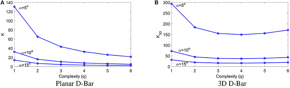
Figure 10. Stiffness of the planar and 3D versions of the D-Bar. (A) Planar D-Bar. (B) 3D D-Bar.
From Figure 10A, it can be seen that the stiffness of the planar D-Bar increases as the complexity, q, and angle α decreases. This is reasonable since as the angle and complexity decreases, the bars participate more and more in the load bearing. Thus the rigidity of the bars increases the stiffness of the structure in the horizontal direction.
From Figure 10B, similar to the planar D-Bar, the stiffness of the 3D configuration increases as angle α decreases. However, in contrast to the planar D-bar, the stiffness K of the structure decreases for the first few self-similar iterations then starts to increase again. Such behavior difference is due to the number of the strings added to the structure. In contrast to the planar tensegrity structure, the number of the strings in the 3D case increases as times more for each iteration step compared to the planar D-Bar.
Example 6: In this example, we calculate the stiffness values of the planar and 3D D-Bar structures presented in example 4. The stiffness of a string is given by Equation (28). If all the parameters given in example 4 are substituted back to Equation (28), the stiffness of one string is found as k = 177N/mm. Given the minimal mass design q = 4 and α = 10° with μ = 0.30, the value of the K is found as 1366N/mm. Evaluation of the K3D is also similar to the planar configuration. The string stiffnesses for the 3D D-Bar are calculated by substituting i instead of q for each complexity level i and substituting ki in Equation (52), we get:
Substituting for the force F = 1000N, α = 10°, L = 0.25m, and minimal mass complexity q = 10 where μ3D = 0.36, the resultant stiffness becomes K = 501N/mm. The minimal mass planar D-Bar has 3 times the stiffness of the minimal mass 3D D-Bar.
Lemma 3: Let angle α and complexity q be equal for planar and 3D D-Bar. The minimum mass design of the planar and 3D D-Bars lead to same global stiffnesses K and K3D formulated as:
Proof: Equation (53) gives the global stiffness K3D of the 3D D-Bar. Recalling the global stiffness formula given in Equation (45) and substituting the individual string stiffness k with the minimal string stiffness given in Equation (28) expression presented in Equation (54) is found. This concludes the proof.
In this section, mass calculation of the planar D-bar subject to stiffness requirement, when ∀αi = α and ∀ki = k, is presented. The mass of a string at complexity level i is given by:
where cross sectional area and Es is the elastic modulus of the string material. From Equation (45), we can write:
Thus, total string mass mst can be written as:
The bar masses should be calculated by checking the primary mode of failure. Inequality (6) is used to evaluate if buckling or yielding is the primary mode of failure. Equations (58) and (59) present mass of the bars for buckling condition and yielding condition, respectively.
The total mass of the structure is given as m = mbar + mst.
Example 7: This example shows a procedure to design a minimal mass planar D-Bar for a fixed global stiffness K = 500N/mm. The materials, force, and size are picked exactly as given in example 4.
Equation (28) gives the minimum stiffness, kmin of strings to avoid yielding. To find the minimal mass solution to satisfy the required K value a search algorithm is summarized below.
We start with complexity one and search for all the α values in small increment till α = 29.477°. We choose the angle to get closest possible k ≥ kmin to get the string mass and check for the failure mode for bars and design them accordingly. We repeat the procedure for the higher complexities till we get the minimum possible mass.
Table 2 gives the complexity, corresponding angle, mode of failure and the mass of the D-Bar which satisfies the desired global stiffness value K = 500N/mm. We observe that the primary mode of failure changes from buckling to yielding after complexity q = 4. The minimum mass design is complexity q = 5 with an angle of α = 14.12°.
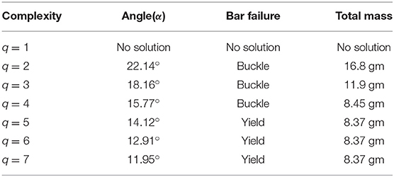
Table 2. Mass of the D-Bar satisfying K = 500N/mm.
Applications of the D-Bar can be extended by combining the D-Bar with other tensegrity structures such as T-Bar. T-Bar offers better mass efficiency than the D-Bar (Skelton and de Oliveira, 2009) and D-bar provides deployability. Hence by combining the D-Bar and T-Bar, it is possible to generate a tensegrity configuration where T-Bar contributes to the mass efficiency and D-Bar contributes to deployability. Figure 11 shows a T-bar under compressive load. This structure has proven to be more mass efficient than D-bar (Skelton and de Oliveira, 2009). The strings in T-bar structure are prestressed to avoid global buckling.
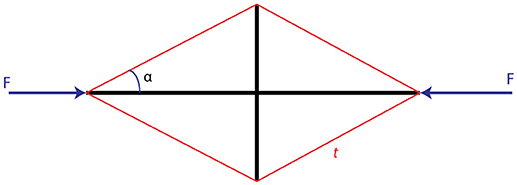
Figure 11. T-bar configuration.
Self-similarity can also be used for T-bars to minimize the mass. If the self-similarity approach is implemented n times, and at the nth iteration instead of the T-Bar, a D-bar unit is used for the self-similar step, the new structure would have complexity q = n + 1 with n level of T-bar units and 1 level of D-bar unit. We name such structure as TnD1 Bar which combines the mass efficiency of T-Bar with the deployability of D-Bar. Figure 12 shows the structural configuration for complexity 4, T3D1 Bar structure with T-Bar angle of αti for each complexity level of i = 1 to n and the D-Bar angle of the αd.
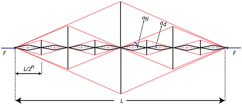
Figure 12. TD-bar configuration.
For the TnD1 Bar, the serially connected D-Bars are the structural members which resist the compressive loading and the strings inherited from the T-Bar iterations provide global stiffness to the structure.
The structure under the compressive loading is, in fact, nothing but a 2n complexity 1 D-Bar units connected in series and the vertical bars of the T-Bar fractals support the connection between two serially connected D-Bars. Following the approach presented in Skelton and de Oliveira (2009), the minimal mass formulation of the TnD1 bar under the buckling condition becomes:
where ϵ is defined in Equation (2) and if ∀αti = αt, then Equation (60) gives:
As explained in section 2, the primary mode of the failure for the minimal mass design should be checked as the number of self-similar iterations increase. With a simple modification of Equation (6), the condition from buckling to yielding failure for the D-Bars of the TnD1 is found as:
The same condition for the vertical bars of TnD1 configuration at the ith complexity level is given as:
If the failure mode of the bars become yielding, the normalized mass ratio (μTD) given in Equations (60) and (61) are no longer valid. Let iy represent the complexity level of the T−Bar fractals for which vertical bars yield and let qy represent the complexity where bars of the D-Bars yield. For a given complexity q, if q < qy but q ≥ iy + 1, the mass ratio becomes:
In addition, if q > qy, the normalized mass ratio becomes:
Similarly, ∀αti = αt, Equations (64) and (65) give:
Practical design of the 3D TD-Bar requires delicate handling of the angles of self-similar T-Bar and D-Bar components due to the possibility of entanglement. This can be avoided by setting the angles at each self-similar level strictly less or equal to that of the previous self-similar iterations at the cost of minimum mass.
Example 8: Consider a TnD1 bar which has a length of L = 10m, angles of and a compressive load of F = 1000N. The materials are selected as given in Table 1. Figure 13 shows the mass ratio of the configuration as the complexity of the structure increases.
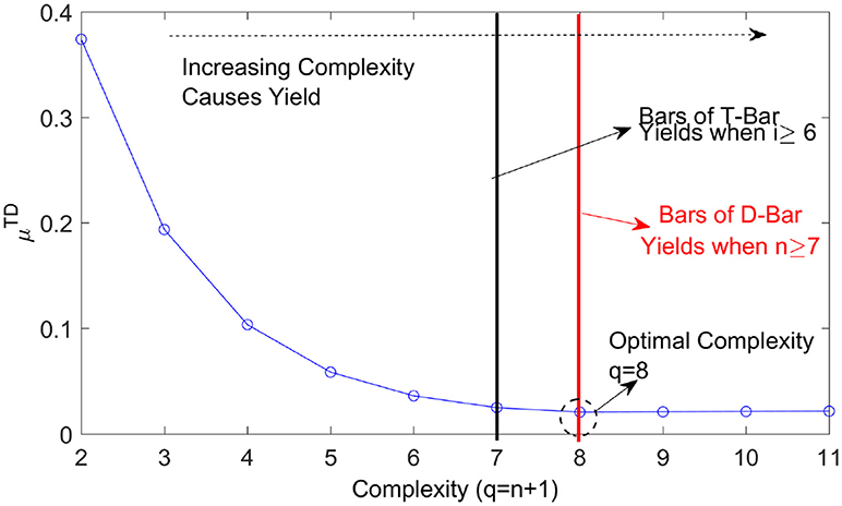
Figure 13. Mass ratio of the configuration vs. the complexity of the structure.
Two vertical lines in the graph represent the change in the primary mode of failure from buckling to yielding. As shown in the figure above T7D1 turned out to be the optimum mass configuration for the given load and length of the structure.
Besides the normalized mass ratio, the gain relations described in section 2 are modified for TnD1 bar as:
Furthermore, the stiffness of the TnD1 bar is also given as
Equation (71) is the equivalent stiffness of the 2n serially connected D-Bars with the approximated stiffness formulation derived in Equation (45).
It is possible to simplify further if αd ≈ αd0. Using the procedure described in section 4 for αd = αd0 + h, the reduces to
Example 9: For the TnD1 bar designed in example 8, the gains are and is 5.6. For the calculation the stiffness of the string, kd must be known. Adopting the similar approach as presented for the derivation of Equation (28), kd is given by:
and for this example, it takes the value of kd = 569N/mm leading to . Stiffness of the TnD1 bar is also calculated as KTD = 143N/mm.
Consider a deployable support structure composed of D-Bars to orient a host with 4 different segments, S1, S2, S3, and S4 as depicted in Figure 14. In this example, there are 5 discrete segments and 5 D-Bars are used to support and orient them. Each segment has a mass of m = 100kg and a length of Ls = 0.25m. The initial length l0 of all D-Bars are equal to 0.25m as shown in Figure 14. The materials selected are as given in Table 1.
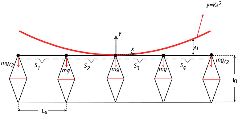
Figure 14. Problem Description for the deployable support structure.
When the final configuration is achieved by deploying all the D-Bars to their desired positions, the angle α of all D-Bars are 10°. When deployed, edges of each segment are required to trace the curve y = Kx2. The origin of the coordinate system is chosen as the symmetry axis of the parabolic surface function and the weights of each segment are shared by D-Bars attached to their edges. The purpose is to minimize the masses of the all D-Bars considering the weight of the platform and design them to generate enough ΔL to satisfy the final shape requirement.
Section 2 shows the mass ratio μ for the minimal mass D-Bar for buckling condition. In this example, each D-Bar would have their own optimal configuration in terms of mass efficiency to satisfy the extension requirement ΔL. Thus, the complexities and angles of each D-Bar may be different. The symmetry of the structure allows to focus on the design of D-Bars for one half and extend the analysis to cover the whole. Thus, by defining a queue number i where i is 1 at the center and goes to i = 3 at the corner, minimal mass of a D-Bar satisfying buckling constraint is given by:
If the bar lengths get small and yielding becomes the primary mode of failure, then the mass of D-Bar becomes:
where angle α0i is the initial angle of the ith D-Bar. Using the geometrical relations, it is possible to relate cos α0i to final desired configuration angle α as:
The ΔLi in Equation (76) is the length change requirement on the ith D-Bar and is a function of the corresponding xi coordinate. Since the length Ls should be conserved, the xi of the ith D-Bar becomes the real positive root of the following polynomial satisfying the inequality xi > xi−1:
After the xi for the ith D-Bar is substituted to the parabolic shape equation y = Kx2, the ΔLi of the ith D-Bar becomes . Substituting Equation (76) back to Equations (74) and (75), we get:
Total mass of all the D-Bars is found as
Substituting for K = 0.35 and i = 1, 2, and 3, the masses of each individual D-Bar are evaluated for the complexity span between q = 1⋯10. Figure 15 shows the variation in mass of each individual D-Bar with increasing complexity.
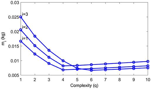
Figure 15. Mass of ith D-Bar changing with complexity.
From Figure 15, the optimal complexities for the 1st and 2nd D-Bars are same whereas the optimal complexity of the 3rd D-Bar is higher. Please note that the mass values are not same for the same complexity D-Bars because of the different α0i. The optimal complexities, angles and the masses of each D-Bar are shown in the Table 3.
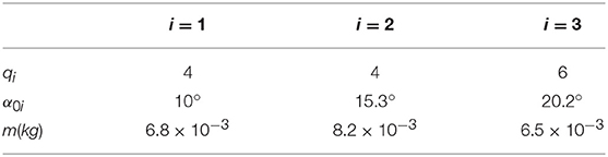
Table 3. Optimal Complexities (qi), angles(α0i), and masses(mi) of ith D-Bar.
Note that as the D-Bar is located toward the edge, the angles of the initial position becomes higher and higher. This is due to the fact that, as previously described in the theorem 1, the longer length changes require higher values of initial angles. The total mass using the formula given in Equation (79) becomes 36.2 grams. Figure 16 shows the final configuration of the structure after the D-Bars generate ΔL.
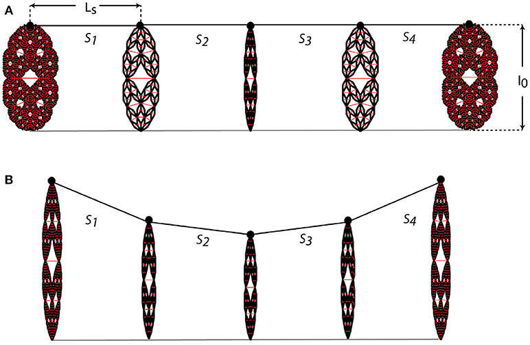
Figure 16. Deployable support structure. (A) Initial configuration, (B) Deployed configuration.
The gain and stiffness values of the D-Bars supporting the structure are calculated for the angle and complexity information given in Table 3. Table 4 shows those values for the initial and final configurations of ith D-Bar.
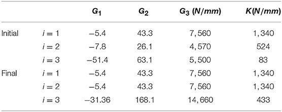
Table 4. Values of the gains and stiffness of the D-Bars for initial and final configurations.
It should be noticed from Table 4 that since there is no deformation on the D-Bar at the center, it will keep its gain relations and stiffness constant. The gain and stiffness change between initial and final configurations gets higher as the D-Bar gets closer to the edges. This is due to increasing angular change during deployment. As explained before, the gains and stiffness values are nonlinear functions of the complexity and angles. Thus, during the design phase, if gains and stiffness values should have a specific value or range, careful evaluation of the problem to satisfy such requirements is necessary.
This paper designs tensegrity D-Bar systems that can serve either of these functions: (i) sensors to measure displacements, (ii) sensors to measure force, (iii) actuators to control displacement, (iv) actuators to control force applied, (v) minimal mass compressive structures subject to a stiffness requirement, and (vi) deployable structures that are efficient in compressive loads. To facilitate such designs, new analytical formulas are derived to give the system a specified displacement gain or force gain, or stiffness requirement.
First, an approach is developed to use the D-Bar for sensing applications. In this case, three different gain relations between the environment and the structural parameters are defined. It is shown that by using the self-similarity approach, it is possible to increase the gain value of the structure leading to the lower tensions and displacements on the strings. Furthermore, by changing the angle of the D-Bar, it is possible to increase or decrease the magnitude of the gains for the D-Bar. It is also shown that for displacement measurement, the angle α should be high whereas the force measurement case requires lower angle α for the higher magnitude of the gain.
Second, the stiffness analysis for the planar and 3D D-Bar systems are analyzed separately for their global stiffness under compressive loading condition. It is shown that as the angle α decreases, the stiffness increases for any complexity. This observation is valid for both the planar and 3D configurations. However, the stiffness behavior of the 3D D-bar system differs from the planar case for the increasing complexity. The increase in the number of the strings for 3D configuration dominates the stiffness formulation after a few self-similar steps and the stiffness tends to increase with the complexity in contrast to the planar configuration. Third, the mass of the planar D-Bar is derived subject to global stiffness requirements. However, checking the stiffness is not enough for this case. The yield condition for the strings should also be considered for the mass calculation of the strings.
Finally, a structure combining the D-Bar and the T-Bar is presented. The aim of such combination is to utilize both the minimal mass property of the T-Bar and the deployable property of the D-bar. The overall analysis showed that the TnD1 system can be employed as a deployable structure functioning as a sensor, actuator or both while satisfying a stiffness requirement and providing an optimum mass solution. Using these results, the paper shows how to design loaded platforms that can deploy to a specified shape while guaranteeing a specified stiffness and minimizing mass.
UB contributed to analytical calculations, generation of the examples and critical reading. RG contributed to generation of examples, critical reading and proofreading of the analytical expressions. RES contributed to development of the sensor/actuator concept and critical reading.
The authors declare that the research was conducted in the absence of any commercial or financial relationships that could be construed as a potential conflict of interest.
Calladine, C. R. (1978). Buckminster Fuller's tensegrity structures and Clerk Maxwell's rules for the construction of stiff frames. Int. J. Solids Struct. 14, 161–172. doi: 10.1016/0020-7683(78)90052-5
Fuller, R., Applewhite, E., and Loeb, A. (1975). Synergetics; Explorations in the Geometry of Thinking. London: Macmillan.
Goyal, R., Bryant, T., Majji, M., Skelton, R., and Longman, A. (2017). “Design and control of growth adaptable artificial gravity space habitats,” in AIAA SPACE and Astronautics Forum and Exposition (Orlando, FL), 5141. doi: 10.2514/6.2017-5141
Goyal, R., and Skelton, R. E. (2018). “Dynamics of class 1 tensegrity systems including cable mass,” in 16th Biennial ASCE International Conference on Engineering, Science, Construction and Operations in Challenging Environments (Cleveland, OH), 868–876. doi: 10.1061/9780784481899.082
Hagiwara, Y., and Oda, M. (2010). “Transformation experiment of a tensegrity structure using wires as actuators,” in Mechatronics and Automation (ICMA), 2010 International Conference on (Xi An), 985–990.
Koizumi, Y., Shibata, M., and Hirai, S. (2012). “Rolling tensegrity driven by pneumatic soft actuators,” in Robotics and Automation (ICRA), 2012 IEEE International Conference on 1988–1993. doi: 10.1109/ICRA.2012.6224834
Motro, R. (2011). Structural morphology of tensegrity systems. Meccanica 46, 27–40. doi: 10.1007/s11012-010-9379-8
Murakami, H., and Nishimura, Y. (2001). Static and dynamic characterization of regular truncated icosahedral and dodecahedral tensegrity modules. Int. J. Solids Struct. 38, 9359–9381. doi: 10.1016/S0020-7683(01)00030-0
Pellegrino, S. (1986). Mechanics of Kinematically Indeterminate Structures. PhD thesis, University of Cambridge.
Rimoli, J. J. (2016). “On the impact tolerance of tensegrity-based planetary landers,” in 57th AIAA/ASCE/AHS/ASC Structures, Structural Dynamics, and Materials Conference (San Diego, CA), 1511.
Skelton, R. (2005). “Dynamics and control of tensegrity systems,” in IUTAM Symposium on Vibration Control of Nonlinear Mechanisms and Structures (Munich: Springer), 309–318.
Skelton, R., and Longman, A. (2014). “Growth capable tensegrity structures as an enabler of space colonization,” in AIAA Space 2014 Conference and Exposition (San Diego, CA), 4370.
Skelton, R. E., and de Oliveira, M. C. (2010). Optimal tensegrity structures in bending: the discrete michell truss. J. Franklin Inst. 347, 257–283. doi: 10.1016/j.jfranklin.2009.10.009
Snelson, K. D. (1965). Continuous tension, discontinuous compression structures. US Patent 3,169,611.
Sultan, C., and Skelton, R. (2004). A force and torque tensegrity sensor. Sens. Actuat. 112, 220–231. doi: 10.1016/j.sna.2004.01.039
Keywords: tensegrity, D-bar systems, stiffness, actuators, sensors
Citation: Boz U, Goyal R and Skelton RE (2018) Actuators and Sensors Based on Tensegrity D-bar Structures. Front. Astron. Space Sci. 5:41. doi: 10.3389/fspas.2018.00041
Received: 08 May 2018; Accepted: 26 November 2018;
Published: 13 December 2018.
Edited by:
Behcet Acikmese, University of Washington, United StatesReviewed by:
Shu Yang, Northwestern Polytechnical University, ChinaCopyright © 2018 Boz, Goyal and Skelton. This is an open-access article distributed under the terms of the Creative Commons Attribution License (CC BY). The use, distribution or reproduction in other forums is permitted, provided the original author(s) and the copyright owner(s) are credited and that the original publication in this journal is cited, in accordance with accepted academic practice. No use, distribution or reproduction is permitted which does not comply with these terms.
*Correspondence: Robert E. Skelton, Ym9ic2tlbHRvbkB0YW11LmVkdQ==
Disclaimer: All claims expressed in this article are solely those of the authors and do not necessarily represent those of their affiliated organizations, or those of the publisher, the editors and the reviewers. Any product that may be evaluated in this article or claim that may be made by its manufacturer is not guaranteed or endorsed by the publisher.
Research integrity at Frontiers
Learn more about the work of our research integrity team to safeguard the quality of each article we publish.