 Alexey G. Butkevich
- Department of Fundamental Astronomy, Pulkovo Observatory (RAS), Saint Petersburg, Russia
High-precision observations require accurate modeling of secular changes in the orbital elements in order to extrapolate measurements over long time intervals, and to detect deviation from pure Keplerian motion caused, for example, by other bodies or relativistic effects. We consider the evolution of the Keplerian elements resulting from the gradual change of the apparent orbit orientation due to proper motion. We present rigorous formulae for the transformation of the orbit inclination, longitude of the ascending node and argument of the pericenter from one epoch to another, assuming uniform stellar motion and taking radial velocity into account. An approximate treatment, accurate to the second-order terms in time, is also given. The proper motion effects may be significant for long-period transiting planets. These theoretical results are applicable to the modeling of planetary transits and precise Doppler measurements as well as analysis of pulsar and eclipsing binary timing observations.
1. Introduction
Keplerian orbits are among the most important concepts in astronomy. Variations of the parameters of a Keplerian orbit lead to various phenomena in observational data. Observed orbit characteristics can vary due to physical or geometrical effects. In the classical two-body problem, when two isolated bodies, possessing centrally symmetric distribution of mass, attract each other according to the Newtonian law, the bodies move about the common center of mass in elliptical orbits. The orbits preserve their form and orientation until the underlying assumptions of the classical problem hold. If any of these prerequisites is violated, the orbit parameters become variable. It happens, for example, when internal mass distribution of any body deviates from spherical symmetry, or the bodies undergo an action of an external (gravitational or non-gravitational) force, or the effects of general relativity come into play.
The impact of asphericity of the central body on motion of an orbiting low-mass body is considered by Iorio (2011) for stellar motions around the rotating black hole in Sgr A*, and by Renzetti (2013, 2014) for the satellite orbital precession. Kaula (2000) gives a detailed exposition of the perturbations in the Keplerian orbital elements due to the geopotential. Moreover, perturbations of the orbital elements of artificial satellite provide powerful tools for experimental testing of various relativistic effects, such as the Lense-Thirring precession (Iorio, 2012a) and post-Newtonian effects due to the oblateness of the central body (Iorio, 2015).
The generalization of the Keplerian orbital elements in general relativity is comprehensively explained in the textbooks by Kopeikin et al. (2011) and Poisson and Will (2014). The additional quantities, needed to describe deviations from a pure Keplerian motion, are referred to as the post-Keplerian parameters and used in modeling binary pulsar observations (Lorimer and Kramer, 2012) and stellar orbits around massive black holes (Iorio and Zhang, 2017).
It is also worth mentioning that, besides the Newtonian and general-relativistic frameworks, the Keplerian orbital elements are explored in the alternative theories of gravitation. For instance, Adkins and McDonnell (2007) and Chashchina and Silagadze (2008) calculated orbital precession due to perturbations of arbitrary central force. Iorio (2005) studied orbital motion in the framework of the braneworld gravity model. Considering Lorentz-violating standard model extension, Iorio (2012b) demonstrated that the Keplerian parameters undergo secular variation due to the gravitomagnetic acceleration. Furthermore, analysis of the precession of the solar system planets provided constraints on the parameters of the preferred-frame parameters (Iorio, 2014).
The perturbations of the Keplerian orbital elements are widely used for analytical calculation of subtle measurable effects in various fields ranging from geodesy to high-energy astrophysics. For example, they are employed in studying geodetic inter-satellite tracking (Cheng, 2002), in developing relationship between the perturbation of the conventional orbital elements and the perturbations of position and velocity (Casotto, 1993). They also provide a theoretical basis for analytical calculation of the post-Keplerian effect in the radial velocity of binary systems (Iorio, 2017a) and the orbital time shift in binary pulsars (Iorio, 2017b) as well as the effect of the Lense-Thirring precession on BepiColombo mission (Iorio, 2018).
The aim of the present work is to consider the effects of proper motion on the orbital elements due to changing orbit orientation with respect to the line of sight. To study the effects in their purest form, we assume that no other body perturbs the orbit and ignore the effects of general relativity. Moreover, our treatment is based on the assumption that the center of mass moves uniformly at a constant velocity. It is worth noting that this approach was pioneered by van den Bos (1926), who, among other things, derived expressions for the variations in the Keplerian elements due to the proper motion. The effects of the change in orbit orientation due to proper motion have been studied for different classes of astronomical objects and various observation techniques. Kopeikin (1996), who considered the case of a binary pulsar, derived equation governing the variation of the projected semimajor axis and the longitude of the periastron due to proper motion and demonstrated that effect of proper motion on pulsar timing may be significantly larger than the effects from gravitational waves. The theoretical study of proper motion effect on Doppler measurements of binary orbits has been undertaken by Kopeikin and Ozernoy (1999). Rafikov (2009) studied the effects of proper motion on timing of planetary transits. Results of this study indicate that for stars with proper motion at the level 10–100 mas yr−1 the rate of variation of transit duration is comparable or exceeds effects from general relativity or stellar oblateness. However, these works consider only linear, first-order in time, terms of the orbital parameters variation.
In the present paper, we first derive rigorous expressions governing the evolution of the Keplerian parameters and then expand them to second-order terms. We consider an isolated system of two bodies with its center of mass moving at constant velocity. The assumption that the center of mass preserves its velocity (both in value and direction) is referred to as the uniform rectilinear model in what follows. The gradual change of orientation of the orbital ellipses with respect to the line of sight results in secular variation of the relevant Keplerian parameters. It should be mentioned that these variation generally depends not only on the conventional proper motion, i.e., transversal velocity, but also on the radial velocity. The model of the uniform motion enables us to easily include the effect of the radial velocity and other non-linear effects. This paper concerns with binary stars and exoplanetary systems.
The paper is organized as follows. We discuss the orbit specification in section 2. Section 3 presents a uniform rectilinear model of stellar motion and related questions. Section 4 contains an analytical treatment of the time-dependence of the Keplerian parameters. Results and conclusions are summarized in sections 5 and 6.
2. Orbit Specification
The equatorial coordinate system is used throughout this paper, with all relevant quantities referring to the solar system barycenter (SSB). The position of an object on the celestial sphere is conventionally specified by right ascension α and declination δ. In what follows, we use the unit vector from SSB toward δ = +90°; in fact, it represents the polar axis of the equatorial system. Let the unit vector determine the barycentric direction to the object, i.e., the direction along the line-of-sight as seen by an observer at the SSB. The coordinates of the vector are
At any position on the celestial sphere, the local directions of increasing α and δ are specified by the unit vectors and , respectively. The vector is parallel to the celestial equator and, accordingly, normal to the vector , while points to the north celestial pole. These vectors can be equivalently found by means of geometric or differential calculations:
where the angular brackets denote vector normalization, 〈x〉 = x/|x|. The three orthogonal unit vectors constitute the so-called normal triad relative to the equatorial system. The vectors and span the tangent plane at the position . Any direction in the tangent plane is specified by the position angle reckoned from north to east, i.e., counterclockwise from to .
The general consideration of the Keplerian orbits can be found in many books (e.g., Heintz, 1978; Kopeikin et al., 2011; Perryman, 2011). Orbits are conventionally parameterized by means of the six Keplerian elements. The five of these elements, semi-major axis a, eccentricity e, inclination i, longitude of the ascending node Ω, and argument of the pericenter ω, specify the geometry of the orbit. The remaining sixth element, which defines position of the body on the orbit at a specified epoch, is usually represented by the mean anomaly at an initial epoch or, equivalently, by the time of the pericenter passage. The three angles i, Ω, ω describing the orbit orientation with respect to the line of sight are illustrated in Figure 1. The inclination is the angle between the orbital plane and the tangent plane. The orbital motion is prograde, i.e., the apparent motion is in the direction of increasing position angle, if i < π/2, and retrograde (clockwise) if i > π/2. Thus, i = 0 and π correspond to face-on orbits with apparent counterclockwise and clockwise motion, with the orbital angular momentum being antiparallel and parallel to the line of sight, respectively. The orbital and tangent plane intersect along the line of nodes. The point where the star recedes from the observer when it crosses the tangent plane is called the ascending node, whose position angle gives Ω. The argument of the pericenter ω is the angle between the ascending node and the pericenter measured in the direction of the star orbital motion.
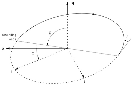
Figure 1. An elliptical orbit as seen by an observer at the solar system barycenter, with the plane of the plot tangent to the celestial sphere. The unit vectors and specify the local directions of increasing equatorial coordinates α and δ. The arrow indicates direction of the orbital motion. i is the inclination of the orbit. The orbit crosses the tangent plane in the two nodes. The ascending node is the node where the object recedes from the observer. The position angle of the ascending node Ω is reckoned counterclockwise from in the tangent plane. The argument of the pericenter ω is the angle between the ascending node and the pericenter measured in the direction of the orbital motion. The orthogonal unit vectors and , with pointing to the pericenter, define the Cartesian coordinates.
To study the effect of proper motion on the orbital parameters, it is convenient to make use of a reference system aligned with the orbit. This system is represented by three orthogonal unit vectors , , , with being parallel to the orbital angular momentum, directed along the semi-major axis from the orbit center to its pericenter, and . The transformation between the right-handed vector triads and is done by the matrix of the direction cosines
This matrix is closely related to the Thiele-Innes elements, another tool for specify orbit orientation (Heintz, 1978; Perryman, 2011). We, however, do not use this formalism in the present paper.
The description by means of the Keplerian elements is equally applicable to all kinds of elliptic orbits. Depending on masses of the bodies, two different cases may be distinguished: objects of comparable masses, such as components of a binary system, or an object revolving around a massive central body, for example, an exoplanet orbiting its host star1. We further address these cases in sections 5.1 and 5.2, respectively.
3. The Uniform Rectilinear Model of Stellar Motion and Transformation of the Normal Triad
A basic assumption of the uniform rectilinear model is that an object moves with constant velocity relative to the SSB. According to this model, the barycentric position of the star at the epoch T is given by the path equation
where b0 is the barycentric position at the initial epoch T0 and v the constant space velocity. For simplicity, we shall subsequently use t = T − T0 as the time argument in all expressions instead of T. Moreover, we use the subscript 0 to denote quantities at t = 0 and omit the time argument in what follows.
The velocity is usually represented as a sum of radial and tangential components
where b0 is the barycentric distance and μ is the proper motion vector:
The asterisk in the notation μα* means that the proper motion in the right ascension contains the factor cosδ: μα* = μαcosδ≡(dα/dt)cosδ. Introducing the radial proper motion, μr = vr/b0, we can write the velocity in the form
Substituting it in Equation (5) and representing the barycentric position as , we obtain the direction vector at the time t:
where fD is the distance factor:
Transformation from one epoch to another is generally referred to as the epoch propagation of astrometric data. For the following, we need the propagations of the two other constituents of the normal triad. To find the vector at the epoch t, we make use of the relation, . After simple, though lengthy, calculations, we find
The normalization factor fP is determined by the condition p2 = 1:
It should be noted that here the proper motion μα does not include the factor cosδ. Finally, substitution of Equations (9) and (11) into the relation gives the propagation of the vector :
These formulae give the complete solution to the problem: they determine the vectors , , and at any instant in terms of their initial values and astrometric parameters. It can be easily seen that the vectors preserve their geometrical properties under this transformation: is always parallel to the celestial equator and always points toward the north celestial pole.
4. Transformation of the Keplerian Elements
4.1. Rigorous Treatment
Equations (11), (13), and (9) describe the time dependence of the normal triad. Combined with the direction cosine matrix given by Equation (4), the latter, in turn, determines propagation of the orbital elements. The resulting equations involve the dot products of the triad constituents and proper motion vector. It is instructive to explicitly write down these products:
The Keplerian elements are conveniently expressed in terms of the direction cosine matrix items. The orbit inclination can be found from
Making use of Equation (9) and substituting the dot products and from Equations (4) and (16), respectively, we find the propagation of the inclination
The argument of pericenter and longitude of the ascending node range from 0 to 2π, therefore both sine and cosine should be known to specify them uniquely. For ω, we take the following two relations
Similarly, substituting from Equation (9), we get the propagation of the argument of the pericenter
Finally, Ω is specified by the relations
Using the vectors and from Equations (11) and (13), we obtain the propagation of the longitude of the ascending node
The above formulae describe the complete transformation of (i0, ω0, Ω0) at epoch T0 into (i, ω, Ω) at the arbitrary epoch T = T0 + t, based on the model of uniform rectilinear stellar motion. It is useful to point out that a reverse transformation from T to T0 is rigorously reversible, i.e., recovers the original parameters, only if the astrometric parameters are propagated to the epoch T (Butkevich and Lindegren, 2014).
4.2. Approximate Formulae
In this section, we derive approximate formulae for the time dependence of the orbital elements to the second order in time. To concisely write the resulting equations, it is convenient to make use of the proper motion position angle ψ; the proper motion components are then
Expanding Equation (18) in a Taylor series in time and keeping the second-order terms, we find the variation of the orbital inclination
Substitution of the propagated inclination from Equation (18) into Equations (21) and (22) and expansion of the results in a series in time gives the change in the argument of the pericenter
Similarly, we obtain the variation of the longitude of the ascending node from Equations (25) and (26). We, however, omit the second order terms because they are very complicated
Here we keep only the linear term for ΔΩ to avoid too length expression. However, the second-order terms of ΔΩ can be easily calculated numerically from the general expressions given by Equations (25) and (26).
The linear terms of the above expressions are derived and discussed in various textbooks and papers (Heintz, 1978; Kopeikin, 1996; Kopeikin and Ozernoy, 1999; Rafikov, 2009). The linear term in Δi and Δω agree with those obtained in other works. However, the situation with ΔΩ is different. The formula for ΔΩ is given only in the book by Heintz (1978) where it was adopted from the pioneering work of van den Bos (1926). Equation (30) contains a term μt cos ψ sin Ω0 cos Ω0 tan δ, which is absent in there. Comparison of our calculation with that work shows that only formula for sin Ω has been used in that paper and the omission of the formula for cos Ω was the reason why the above mentioned term was missing.
Making use of the proper motion position angle ψ enables us to make qualitative conclusions on the evolution of the Keplerian elements. Equation (28) shows that, if the proper motion is along the line of nodes (ψ = Ω0 or ψ = Ω ± π), the linear term in Δi vanishes and the inclination depends on time as ~μ2t2. For the argument of the pericenter, the situation is more interesting: if the proper motion is normal the line of nodes (ψ = Ω0 ± π/2), both the first- and second-order terms are zero and ω becomes independent of time. Moreover, it can be demonstrated that, in such a configuration, ω does not depend on time at all. The linear term of the longitude of the ascending node vanishes only under very special conditions. For example, one may infer from Equation (30) that ΔΩ = 0 when δ = 0 and cos (ψ − Ω0) = 0, i.e., for a star on the celestial equator with proper motion normal to the line of nodes.
The second-order terms of all the orbital elements include the radial proper motion μr. Thus, an accurate treatment of the evolution of the Keplerian parameters needs to take radial velocity as well as the tangential proper motion into account.
4.3. Face-on Orbits
For face-on orbits, the orbit and tangent planes are parallel and the line of nodes cannot be defined, therefore there is an ambiguity in the choice of the angles Ω and ω. Whatever choice is made, these quantities change discontinuously when the orbit plane becomes normal to the line of sight. Mathematically this corresponds to the fact that Equations (29) and (30) have singularities if i = 0. The inclination remains the only Keplerian angle which changes smoothly when the alignment geometry passes through a face-on configuration. However, propagation formulae need some modification for such cases. Substituting i = 0 and π in Equation (18), we find the propagation of the inclination for a face-on orbit
The upper sign applies for prograde motion and the lower sign for retrograde motion. Expansion to the quadratic terms gives
The absolute value in this formulae is related to the fact that the sign of Δi should not change under time reversal, as can be seen from straightforward geometrical arguments.
5. Discussion
In the following, we discuss some practical implications of the analytical results obtained in the preceding sections. Since the first-order proper-motion effects have already been studied in the context of various object type (e.g., Kopeikin, 1996; Rafikov, 2009), we mainly concern the second-order effects. We consider first the impact of the proper motion on the radial velocity amplitude of a binary star component. As a second example, we examine how it affects the duration of exoplanetary transit time.
5.1. Effect on Radial Velocity of Binary Component
Radial velocity amplitudes of components of a binary system depend on the orbit inclination. Let the masses of the components be M1 and M2, then it follows from Kepler's third law that for a circular orbit the radial velocity semi-amplitude of the first component is
where G is the gravity constant and P is the orbital period. Moreover, we introduced to designate the velocity amplitude the star had if the system would be seen edge-on. Making use of the variation of the orbit inclination given by Equation (28), we find the variation of the velocity amplitude
To estimate the size of the effect, we ignore the trigonometric factors and note that both μ and μr are of the order of v/d, the ratio of the space velocity to the barycentric distance. Then the first- and second-order terms can be approximated by and , respectively. Assuming for simplicity that the components are of the same mass M, we find the following estimates for the first-order term
and for the second-order term
These equations vary in the units of the orbital period to emphasize the very large difference between the effects. The linear effect, which may amount to about m s−1 for high-velocity nearby stars, should be taken into account in interpretation of precise Doppler measurements. In contrast, the second-order effect, being at the level of mm s−1 per century even for short-period close binaries, is truly negligible in practice.
5.2. Effect on Timing of Planetary Transits
The effects of proper motion on the timing of planetary transits are studied by Rafikov (2009) in the linear approximation. In what follows, we complement this study by considering the second-order effects. Duration of planetary transit is the time interval during which a planet moves in front of its host star. We consider here the simplest case of a circular orbit and ignore small effects due to planet radius. The transit geometry is conveniently described in terms of the so-called impact parameter, the distance between the center of stellar disc and the projection of the planetary orbit onto it, expressed in units of the stellar radius:
where R is the radius of the host star and a is the radius of the planetary orbit. Variation of the duration due to a change in the orbit inclination lends itself to a straightforward geometrical interpretation. Any increase or decrease of the angle between the line of sight and the orbital plane makes the impact parameter larger or smaller. This, in turn, changes the length of the projection and the time the planet takes to pass through it. The effect of changing inclination on transit duration is evidently larger when the orbit projection lies not very close to the stellar center because small variations of the impact parameter then result is significant changes in the projection length due to the curvature of the stellar disc.
For a circular orbit, with the planetary radius ignored, the transit duration T depends on three parameters: the orbital period P, the ratio of the orbit and stellar radii a/R and the impact factor b (e.g., Perryman, 2011, Chapter 6):
The effect of changing orbit inclination on the transit duration is evidently more pronounced for long-period planets when a small change in inclination can result in a sizeable shift of the orbit projection on stellar disc. As explained above, this effect is especially large for systems with impact factors close to one when transit occurs close to the edge of the stellar disc. On the other hand, the proper motion effect are evidently significant for stars with high-proper motion. To compare the effects of proper motion and orbit period, we considered two opposite cases: a high-proper motion star hosting a short-period planet and a system with moderate proper motion and long-period planet. The first case is well exemplified by GJ 436b, a Neptune-mass planet with P = 2.644 day orbiting an M dwarf star with μ = 1, 210 mas yr−1 (Torres et al., 2008). To illustrate a long-period system, we considered a planet with P = 1 yr orbiting a Solar-type star with μ = 72 mas yr−1. Moreover, to demonstrate strong dependence of grazing transit on time, we assume that the impact factor is close to unity, b = 0.975. Parameters of these transiting systems are summarized in Table 1.
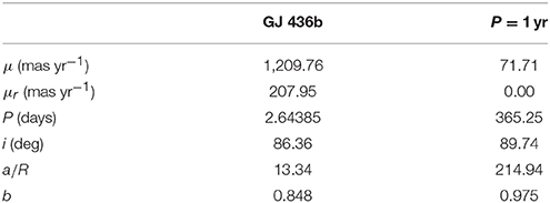
Table 1. Parameters of the transiting planets.
The evolution of transit duration was calculated for a time span of 25 years for both systems. The results of the numerical calculations are shown in Figures 2, 3. The plots also contain separate graphs showing the second-order effects. Practical significance of these effects is determined on the accuracy of transit timing, σT. Assuming σT = 10 s , we see that the linear effects are significant for time interval ≥15 yr, while the second-order effects are negligible for GJ 436b. In contrast, for a planet with P = 1 yr, the linear effects should be measurable in successive transits, whereas the the second-order effect are important for t ≃ 30 yr. However, the situation changes if higher timing is attainable. For example, the quadratic variation of the transit duration should be taken into account for t ≃ 22 yr if σT = 5 s and for t ≃ 10 yr if σT = 1 s. Thus, we may conclude that the linear effect may be significant for long-period planets, because variation of the transit duration between two subsequent transit events can be measured in practice for such systems. The second-order effect are important for grazing transits, provided that the timing accuracy is better than ≃ 10 s.
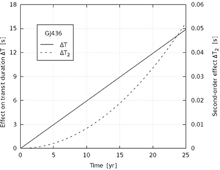
Figure 2. Effect of proper motion on the transit planet GJ 436b. The solid line and left axis show the difference in the duration of transit, while the dashed line and right axis show the second-order term.

Figure 3. As Figure 2, but for a system with μ = 71 mas yr−1, cosi = 89.°74 and P = 1 yr.
6. Conclusions
We have presented an analysis of the effect of proper motion on the Keplerian orbital elements. Change in the orbit orientation due to the star's space motion leads to variation of the three Keplerian elements, which specify the alignment geometry: inclination, longitude of the ascending node, and argument of the pericenter. The uniform rectilinear model of barycentric stellar motion provides the time-dependence of the normal triad. Resolving the unit vectors associated with the orbits along the triad constituents, we derived explicit and rigorous formulae for the secular variation of the three Keplerian parameters. It should be emphasized that the effects studied in this paper are purely kinematical with no post-Newtonian acceleration taken into account.
The analysis of the obtained results demonstrated that a consistent treatment of the evolution of the orbital parameters necessitates the accounting for all components of the star velocity. The conventional proper motion, i.e., the tangential velocity component, is sufficient only in the linear approximation. In the second-order terms in time, however, the radial velocity comes into play. The effect of the radial velocity on the Keplerian elements, , is equivalent to the secular, or perspective, acceleration, a well-known effect in classical astrometry. Numerical estimations indicate that the proper motion may provide significant effect on transit timing variations for long-period planets with grazing transit. The results of this study are applicable to modeling of planetary transits and precise Doppler measurements as well as analysis of pulsar and eclipsing binary timing observations.
Author Contributions
The author confirms being the sole contributor of this work and approved it for publication.
Conflict of Interest Statement
The author declares that the research was conducted in the absence of any commercial or financial relationships that could be construed as a potential conflict of interest.
Acknowledgments
The author is very much indebted to the reviewers for their valuable comments and suggestions that have greatly improved an initial version of the paper. This research has made use of the VizieR service and of the SIMBAD database, both operated at CDS, Strasbourg, France, as well as of NASA's Astrophysics Data System, the Exoplanet Orbit Database (Han et al., 2014) and the Exoplanet Data Explorer at exoplanets.org.
Footnotes
1. ^Rigorously speaking, both the host star and planet orbit the system's center of mass, but the amplitude of the stellar orbital motion is very small compared to that of the planet because of the significant difference in mass. It worth mentioning that analysis of the reflex motion of the host star is fundamental in astrometric detection of exoplanets and other unseen companions (Perryman, 2011; Butkevich, 2018).
References
Adkins, G. S., and McDonnell, J. (2007). Orbital precession due to central-force perturbations. Phys. Rev. D 75:082001. doi: 10.1103/PhysRevD.75.082001
Butkevich, A. G. (2018). Astrometric detectability of systems with unseen companions: effects of the earth orbital motion. Month. Not. R. Astron. Soc. 476, 5658–5668. doi: 10.1093/mnras/sty686
Butkevich, A. G., and Lindegren, L. (2014). Rigorous treatment of barycentric stellar motion. Astron. Astrophys. 570:A62. doi: 10.1051/0004-6361/201424483
Casotto, S. (1993). Position and velocity perturbations in the orbital frame in terms of classical element perturbations. Celestial Mech. Dyn. Astr. 55, 209–221. doi: 10.1007/BF00692510
Chashchina, O. I., and Silagadze, Z. (2008). Remark on orbital precession due to central-force perturbations. Phys. Rev. D 77:107502. doi: 10.1103/PhysRevD.77.107502
Cheng, M. (2002). Gravitational perturbation theory for intersatellite tracking. J. Geod. 76, 169–185. doi: 10.1007/s00190-001-0233-6
Han, E., Wang, S. X., Wright, J. T., Feng, Y. K., Zhao, M., Fakhouri, O., et al. (2014). Exoplanet orbit database. II. Updates to Exoplanets.org. PASP 126:827. doi: 10.1086/678447
Iorio, L. (2005). On the effects of Dvali-Gabadadze-Porrati braneworld gravity on the orbital motion of a test particle. Class. Quant. Gravit. 22, 5271. doi: 10.1088/0264-9381/22/24/005
Iorio, L. (2011). Perturbed stellar motions around the rotating black hole in Sgr A* for a generic orientation of its spin axis. Phys. Rev. D 84:124001. doi: 10.1103/PhysRevD.84.124001
Iorio, L. (2012a). General relativistic spin-orbit and spin–spin effects on the motion of rotating particles in an external gravitational field. Gen. Relat. Gravit. 44, 719–736. doi: 10.1007/s10714-011-1302-7
Iorio, L. (2012b). Orbital effects of Lorentz-violating standard model extension gravitomagnetism around a static body: a sensitivity analysis. Class. Quant. Gravit. 29:175007. doi: 10.1088/0264-9381/29/17/175007
Iorio, L. (2014). Constraining the preferred-frame α1, α2 parameters from solar system planetary precessions. Int. J. Mod. Phys. D 23:1450006. doi: 10.1142/S0218271814500060
Iorio, L. (2015). Post-newtonian direct and mixed orbital effects due to the oblateness of the central body. Int. J. Mod. Phys. D 24:1550067. doi: 10.1142/S0218271815500674
Iorio, L. (2017a). Post-Keplerian effects on radial velocity in binary systems and the possibility of measuring General Relativity with the star S2 in 2018. Month. Not. R. Astron. Soc. 472, 2249–2262. doi: 10.1093/mnras/stx2134
Iorio, L. (2017b). Post-Keplerian perturbations of the orbital time shift in binary pulsars: an analytical formulation with applications to the galactic center. Eur. Phys. J. C 77:439. doi: 10.1140/epjc/s10052-017-5008-1
Iorio, L. (2018). Analytically calculated post-Keplerian range and range-rate perturbations: the solar Lense-Thirring effect and BepiColombo. Month. Not. R. Astron. Soc. 476, 1811–1825. doi: 10.1093/mnras/sty351
Iorio, L., and Zhang, F. (2017). On the post-keplerian corrections to the orbital periods of a two-body system and their application to the galactic center. Astrophys. J. 839:3. doi: 10.3847/1538-4357/aa671b
Kaula, W. M. (2000). Theory of Satellite Geodesy: Applications of Satellites to Geodesy. New York, NY: Dover Publications.
Kopeikin, S., Efroimsky, M., and Kaplan, G. (2011). Relativistic Celestial Mechanics of the Solar System. Weinheim: Wiley-VCH.
Kopeikin, S. M. (1996). Proper motion of binary pulsars as a source of secular variations of orbital parameters. Astrophys. J. 467, L93–L95.
Kopeikin, S. M., and Ozernoy, L. M. (1999). Post-newtonian theory for precision Doppler measurements of binary star orbis. Astrophys. J. 523, 771–785.
Lorimer, D. R., and Kramer, M. (2012). Handbook of Pulsar Astronomy. Cambridge: Cambridge University Press.
Poisson, E., and Will, C. M. (2014). Gravity: Newtonian, Post-Newtonian, Relativistic. Cambridge: Cambridge University Press.
Rafikov, R. R. (2009). Stellar proper motion and the timing of planetary transits. Astrophys. J. 700, 965–970. doi: 10.1088/0004-637X/700/2/965
Renzetti, G. (2013). Satellite orbital precessions caused by the octupolar mass moment of a non-spherical body arbitrarily oriented in space. J. Astrophys. Astron. 34, 341–348. doi: 10.1007/s12036-013-9186-4
Renzetti, G. (2014). Satellite orbital precessions caused by the first odd zonal j3 multipole of a non-spherical body arbitrarily oriented in space. Astrophys. Space Sci. 352, 493–496. doi: 10.1007/s10509-014-1915-x
Torres, G., Winn, J. N., and Holman, M. J. (2008). Improved parameters for extrasolar transiting planets. Astrophys. J. 677:1324. doi: 10.1086/529429
Keywords: stellar kinematics, binary stars, analytical methods, pulsars, exoplanetary systems
Citation: Butkevich AG (2018) Proper Motion and Secular Variations of Keplerian Orbital Elements. Front. Astron. Space Sci. 5:18. doi: 10.3389/fspas.2018.00018
Received: 31 January 2018; Accepted: 30 April 2018;
Published: 23 May 2018.
Edited by:
Alessandra Celletti, Università degli Studi di Roma Tor Vergata, ItalyReviewed by:
Lorenzo Iorio, Ministry of Education, Universities and Research, ItalyBalint Erdi, Eötvös Lorànd University, Hungary
Catalin Bogdan Gales, Alexandru Ioan Cuza University, Romania
Copyright © 2018 Butkevich. This is an open-access article distributed under the terms of the Creative Commons Attribution License (CC BY). The use, distribution or reproduction in other forums is permitted, provided the original author(s) and the copyright owner are credited and that the original publication in this journal is cited, in accordance with accepted academic practice. No use, distribution or reproduction is permitted which does not comply with these terms.
*Correspondence: Alexey G. Butkevich, YWcuYnV0a2V2aWNoQGdtYWlsLmNvbQ==