Talbot-Lau devices: a reappraisal

The Talbot effect and the Lau effect have been usefully applied in optical interferometry, and for designing novel X-ray devices, as well as for implementing useful instruments for matter waves. In temporal optics, the above phenomena play a significant role for reconstructing modulated, optical short pulses that travel along a dispersive medium. We note that the Talbot-Lau devices can be spatial frequency tuned if one employs varifocal lenses as a nonmechanical technique. Thus, we identify a pertinent link between the Talbot-Lau sensors and the development of artificial muscle materials, for generating tunable lenses. Our discussion unifies seemly unrelated topics, for providing a global scope on the applications of the Talbot-Lau effect.

1 Introduction

The self-imaging phenomenon is a fundamental property of the diffraction patterns generated by periodic structures. In several ranges of the electromagnetic spectrum, as well as in matter waves, the self-imaging phenomenon has found a myriad of applications. We recognize that a reappraisal on the subject is not a simple task. Despite their importance, we decided to leave out the publications on X-rays, nonlinear optics, and quantum optics (Bachche et al., 2017; Bouffetier et al., 2020; Deng et al., 2020; Dennis et al., 2007; Morimoto et al., 2020; Nikkhah et al., 2018; Neuwirth et al., 2020; Hall et al., 2021; Gerlich et al., 2007; Wen et al., 2013). Here, we focus in the applications on the optical range, by noticing the usefulness of the self-imaging phenomena in optical interferometry (Lau, 1948; Yokozeki and Suzuki, 1971a; Yokozeki and Suzuki, 1971b; Lohmann and Silva, 1971; Lohmann and Silva, 1972; Bartelt and Jahns, 1979; Jahns and Lohmann, 1979; Bartelt and Li, 1983; Bolognini et al., 1985; Ojeda-Castañeda et al., 1988; Ibarra and Ojeda-Castañeda, 1993), for implementing novel optical sensors (Silva, 1971; Chavel and Strand, 1984; Nakano and Murata, 1985; Chang and Su, 1987; Bernardo and Soares, 1988; Su and Chang, 1990; Sriram et al., 1992; Gómez-Sarabia et al., 2019), and for setting theta demodulators (Andrés et al., 1986; Ojeda-Castañeda and Sicre, 1986; Chitralekha et al., 1989; Barreiro and Ojeda-Castañeda, 1993; Ojeda-Castañeda et al., 1998). The later type of optical setups leads to the implementation of a noncoherent version of the Abbe-Porter experiments (Ojeda-Castañeda et al., 1989a). We attempt to link the basic theory of unrelated topics, for providing a global scope on the applications of the Talbot-Lau effect. In Section 1, we emphasize the concept of noncoherent superimposition of interference patterns. In Section 2, we identify the similarities and the differences between the Talbot effect with the Lau effect, for discussing a noncoherent version of the Talbot effect (Ojeda-Castañeda et al., 1989b; Gómez-Sarabia and Ojeda-Castañeda, 2023a). In Section 3, we include the use of varifocal lenses, for governing the presence of tunable fractions of the Talbot effect, at a fixed detecting plane. In Section 4, we discuss the use of a linear combination of laterally displaced versions of the initial grating, for describing fractional Talbot images. In Section 5, we discuss briefly modal dispersion for describing the presence of self-images in optical fibers. In Section 6, we discuss a statistical model for relating the average of randomly located Talbot images, with certain optical sensors. In Section 7, for approaching the temporal aspects of the self-imaging phenomenon, we discuss chromatic dispersion in optical fibers.

2 Spatially noncoherent young fringes

We start by referring to the pioneering work of Rogers, who described the use spatially noncoherent light, for obtaining two beam interference patterns, with high visibility (Rogers, 1963). In Figure 1, we depict the principle of the optical setup, which was proposed by Rogers.

FIGURE 1

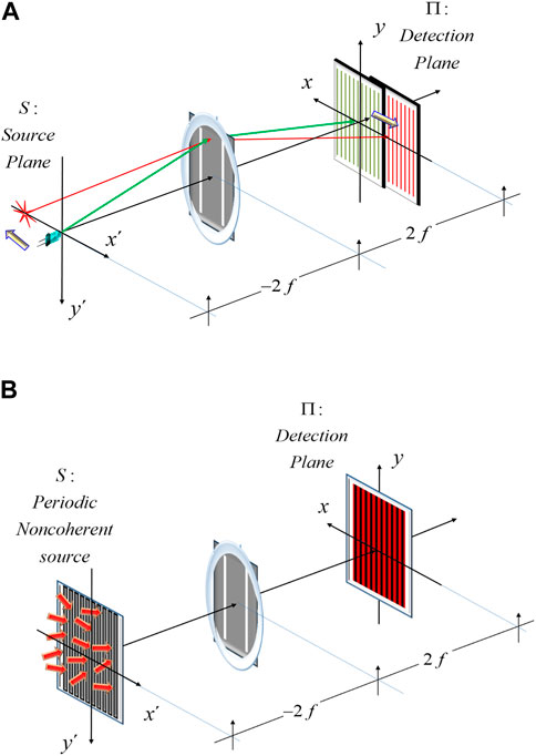
FIGURE 1. Noncoherent superposition of two independent (noncoherent) interference fringes, in the classical optical setup of the two-slit mask. In (A), two independent point sources are shown in distinct color, only to emphasize their contributions. In (B), the several noncoherent sources slits are periodically distributed along the horizontal axis.

As shown in Figure 1, one can superimpose several independent two-slit interferograms. To this end, one employs a spatially noncoherent, periodic source. The extended source has several slits. Each slit shifts laterally an independent interferogram. Here, it is convenient to define the term “in-register.” Each independent interferogram is a sinusoidal irradiance distribution. All the interferograms have the same period and the same modulation. Then, two interferograms are “in-register,” if one of the interferograms is laterally displaced by an integer number of their common period. And consequently, the overall pattern has high visibility. In mathematical terms, let us consider a 1-D model. For the two-slit interferometer with unit magnification, at the detection plane, Π, the irradiance distribution is

$I_{\mathrm{\Pi }}\left(x\right)=\left(\frac{1}{2}\right)\left[1+\cos \left(2\pi \frac{x}{d}\right)\right].(1)$

This irradiance distribution is the irradiance impulse response, of the optical setup in Figure 1. At the source plane, S, we consider a set of mutually noncoherent point sources. Then, the irradiance distribution, at the source plane, S, is

$I_S\left(x´\right)=\left(\frac{1}{2N+1}\right){\displaystyle \sum _{n=-N}^N}\delta \left(x´+np\right).(2)$

Since the optical system is under noncoherent illumination, the final irradiance distribution is

$I\left(x\right)=\underset{-\infty }{\overset{\infty }{{\displaystyle \int }}}{I}_S\left(x´\right)I_{\mathrm{\Pi }}\left(x-x´\right)dx´(3)$

By substituting Eqs. (1, 2) in Eq. (3), we obtain

$I\left(x\right)=\frac{1}{2}+\left(\frac{1}{2N+1}\right){\displaystyle \sum _{n=1}^N}\cos \left[2\pi \frac{x}{d}+2\pi \frac{p}{d}n\right].(4)$

It is apparent from Eq. (4) that for p = L d, where L is a positive integer number, there is an in-register condition. In other words, all the sinusoidal variations overlap at their maxima values.

Of course, the in-register condition is not restricted to the renown Young´s two-slits experiment. In Figure 2, we depict our proposal for achieving in-register interference patterns, when using polarization prisms. The polarizing prisms can generate sinusoidal irradiance distributions, as those described in Eq. (1). For example, for the Wollaston prism in Figure 2A, each element of the source is an illuminating slit, which is spatially noncoherent with any other slit. However, the whole source can have the same polarization state (say, linear polarization at 45°).

FIGURE 2

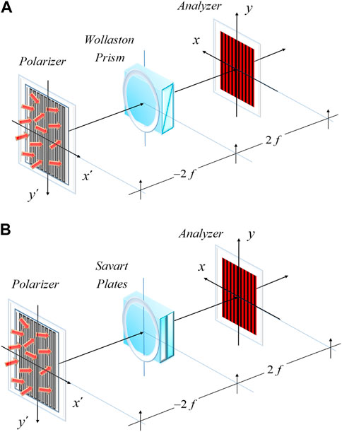
FIGURE 2. Proposed optical setups for superimposing several mutually noncoherent interferograms. However, instead of using the two-slit mask, we employ a polarization device. The noncoherent source is formed by a set of narrow periodic slits. Any two slits are spatially noncoherent. In (A) we use a Wollaston prism. In (B), we employ the Savart plates.

As depicted in Figure 2, let us consider a slit that is located off axis, say by a distance x´ on the source plane. After being collimated by a lens, this slit generates a tilted plane wave, which has linear polarization at 45°. By using the Jones matrix formalism (Shurcliff, 1968), just before impinging on the Wollaston prism, the complex amplitude distribution reads

$E_0\left(x;x´\right)=\left(\frac{\sqrt{2}}{2}\right)\left[\begin{array}{c}1\\ 1\end{array}\right]\exp \left(-i\pi \frac{x´}{\lambda f}x\right).(5)$

In Eq. (5) the lower case, Latin letter, f denotes the focal length of the lens in Figure 2. After crossing the Wollaston prism, the complex amplitude distribution is

$E_1\left(x;x´\right)=\left[\begin{array}{cc}\exp \left(i2\pi \frac{\alpha }{\lambda }x\right)& 0\\ 0& \exp \left(-i2\pi \frac{\alpha }{\lambda }x\right)\end{array}\right]E_0\left(x;x´\right).(6)$

In Eq. (6) the lower case, Greek letter, alpha denotes the wedge angle of the thin components forming the Wollaston prism. And just before the detection plane, a polarizer at an angle of 45° modifies the state of polarization, as follows

$E_2\left(x;x´\right)=\left(\frac{\sqrt{2}}{2}\right)\left[\begin{array}{cc}1& 1\\ 1& 1\end{array}\right]E_1\left(x;x´\right).(7)$

After performing straightforward matrix operations, Eq. (7) can be written as is expressed in Eq. (8)

$E_2\left(x;x´\right)=\left[\begin{array}{c}1\\ 1\end{array}\right]\cos \left(2\pi \frac{\alpha }{\lambda }x\right)\exp \left(-i\pi \frac{x´}{\lambda f}x\right).(8)$

Therefore, at the detection plane the non-normalized version of the irradiance distribution is

$I_2\left(x;x´\right)=2{\cos }^2\left(2\pi \frac{\alpha }{\lambda }x\right).(9)$

Equivalently, Eq. (9) can be written as the irradiance distribution that reads

$I_2\left(x;x´\right)=1+\cos \left(2\pi \frac{2\alpha }{\lambda }x\right).(10)$

We note that Eq. (10) is not normalized. For further details, the reader is kindly addressed to reference (Françon and Mallick, 1971; Gimeno-Gomez et al., 2023). Next, we substitute the irradiance impulse response in the form of sinusoidal fringes, by a binary irradiance impulse response.

3 The noncoherent Talbot effect

Under coherent illumination, the self imaging phenomenon is known as the Talbot effect. And under suitable forms of noncoherent illumination, one can obtain irradiance distributions that have analogous properties to those obtained in the Talbot effect. In the latter case, the self imaging phenomenon is known as the Lau effect. In what follows, we describe mathematically the similarities and the differences between these phenomena. To that end, let us consider as an input object a grating with a binary, amplitude transmittance. The grating is represented by its Fourier series

$g\left(x\right)={\displaystyle \sum _{m=-\infty }^{\infty }}{C}_m\exp \left(i2\pi \left(\frac{m}{d}\right)x\right).(11)$

Under the paraxial regime, it is well-known that at a distance z, the Fresnel diffraction pattern has the following complex amplitude distribution

$\psi \left(x,z\right)={\displaystyle \sum _{m=-\infty }^{\infty }}{C}_m\left[\exp \left(-i\pi \lambda {\left(\frac{m}{d}\right)}^{2}z\right)\right]\exp \left(i2\pi \frac{m}{d}x\right).(12)$

By neglecting the walk-off effect, Eq. (12) can be rewritten in terms of the Talbot distance, Z_T = 2 d²/λ, as follows

$\psi \left(x,z\right)={\displaystyle \sum _{m=-\infty }^{\infty }}{C}_m\left[\exp \left(-i2\pi \left(\frac{z}{Z_T}\right)m^2\right)\right]\exp \left(i2\pi \frac{m}{d}x\right).(13)$

It is apparent from Eq. (13) that if the distance z is an integer multiple of Z_T, the Fresnel diffraction is the self-image of the initial grating. In the following section, we consider that z is a fraction of Z_T. Here, we note that the binary grating reproduces itself. Then, its irradiance distribution is also a binary distribution. Therefore, the irradiance impulse response is

$I_{\mathrm{\Pi }}\left(x\right)={\displaystyle \sum _{m=-\infty }^{\infty }}{C}_m\exp \left(i2\pi \left(\frac{m}{d}\right)x\right).(14)$

Equation (14) is the irradiance distribution of a grating. As depicted in Figure 3, for achieving an in-register superposition, the separation between the point sources must be

$p=\left(\frac{f}{N{Z}_T}\right)d.(15)$

FIGURE 3

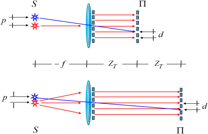
FIGURE 3. Schematics for relating the period, of the mutually noncoherent point sources, with the number N of Talbot self-images.

Equation (15) is the in-register condition. And consequently, Eq. (2) now reads

$I_S\left(x´\right)=\left(\frac{1}{2N+1}\right){\displaystyle \sum _{n=-N}^N}\delta \left(x´+n\left(\frac{f}{N{Z}_T}\right)d\right).(16)$

By substituting Eq. (16) in Eq. (3), we obtain the final irradiance distribution

$I\left(x\right)={\displaystyle \sum _{m=-\infty }^{\infty }}{C}_m\exp \left(i2\pi mn\left(\frac{f}{N{Z}_T}\right)\right)\exp \left(i2\pi \left(\frac{m}{d}\right)x\right).(17)$

From Eq. (17) we claim that the in-register condition leads to a relationship between the focal length, of the collimating lens, with the N-fold self-image

$f=\left(LN\right)Z_T.(18)$

In Eq. 18 the upper-case letter L is an integer number. As depicted in the upper part of Figure 3, the trivial case is obtained if L = 1, and N = 1.

4 Tunable fractional Talbot images

For adding flexibility to the use of self-images, and to the generation of Moiré patterns, Luxmoore proposed a simple technique for controlling the spatial frequency of a master grating (Luxmoore and Dickson, 1971). In Figure 4A, we show an optical setup that reproduces Luxmoore technique. The master grating, with fixed spatial frequency, is illuminated with a divergent beam, and it is displaced along the optical axis. In this manner, one can magnify the virtual Fourier spectrum, which is located at the same plane of the illuminating point source.

FIGURE 4

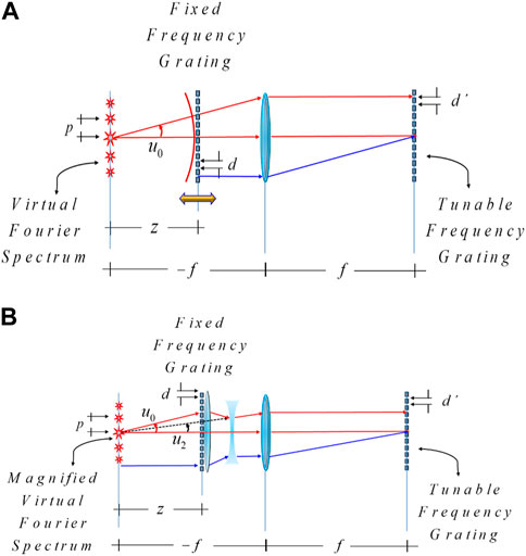
FIGURE 4. Optical setups for tuning the scale of the virtual Fourier spectrum, which consequently controls the generation of a grating with variable spatial frequency. In (A) the optical setup proposed by Luxmoore. In (B) a recently proposed optical setup, which employs two varifocal lenses for implementing a motionless technique.

For the next discussion, it is relevant to note the following. Here, we employ the Fresnel diffraction in the paraxial regime. As noted by Papoulis, the paraxial approximation is valid if the following condition is satisfied (Papoulis, 1968). Let us denote by theta, θ, the angle between the optical axis and the edge of the diffraction mask, which is located at the distance z. One is allowed to use the paraxial regime if

$\theta <{\left(\frac{\lambda }{25z}\right)}^{1/4}.(19)$

That means that for z = λ (2 × 10⁴)/25, the angle theta should be less than 0.05 radians. If at the edge of a grating the height is ten time the period of the grating, 10 d, say with d = 0.1 mm, then θ = (1 (mm)/z (mm)). And consequently, the Fresnel approximation is valid if z > 20 (mm). On the other hand, for specifically describing the Talbot effect, Lohmann (Lohmann and Sinzinger, 1968) has indicated that the paraxial approximation is valid if

$z<\frac{1}{{\lambda }^3}{\left(\frac{d}{m}\right)}^4.(20)$

In Eq. (20), again the lower-case letter “d” denotes the period of the grating (say, 0.1 mm); m is the maximum value of the diffraction order (say, m = 10); and the wavelength is λ = 6.38 × 10⁻⁴ mm. For these values, we obtain that z < 38.5 (mm). Therefore, from Eqs (19, 20), we have that the paraxial approximation is valid if the value of the distance z is located inside the interval 20 (mm) < z < 38.5 (mm). For a non paraxial treatment of the Talbot effect see reference (Cohen-Sabban and Joyeux, 1983). Also in Section 5, there is a non paraxial treatment of self-imaging.

Next, we use the concept of the virtual Fourier spectrum, G(x_s; z) of the master grating. For the optical setup in Figure 4A, at the source plane, the complex amplitude distribution is

$G\left(x_s;z\right)=\underset{-\infty }{\overset{\infty }{{\displaystyle \int }}}\exp \left(-i\pi \frac{{\left(x_s-x´\right)}^2}{\lambda z}\right)\exp \left(i\pi \frac{x{´}^2}{\lambda z}\right)g\left(x´\right)dx´.(21)$

Next, if we substitute Eq. (11) in Eq. (21), we obtain the mathematical expression of a Fourier transformation. For expressing this transform, we employ the Talbot distance, Z_T = 2 d²/λ. Then, we obtain

$G\left(x_s;z\right)={\displaystyle \sum _{m=-\infty }^{\infty }}{C}_m\left[\exp \left(-i2\pi \left(\frac{z}{Z_T}\right)m^2\right)\right]\delta \left(x_s+\frac{\lambda z}{d}m\right).(22)$

Equation (22) represents the complex amplitude distribution of the Fourier spectrum. At the middle of Figure 4, we show a lens with fixed optical power. This element implements optically a Fourier transform, from the source plane to the detection plane. Thus, at the detection plane, we obtain the amplitude impulse response

$\psi \left(x,z\right)={\displaystyle \sum _{m=-\infty }^{\infty }}{C}_m\left[\exp \left(-i2\pi \left(\frac{z}{Z_T}\right)m^2\right)\right]\exp \left(i2\pi \left(\frac{m}{d´}\right)x\right).(23)$

From Eq. (23), we observe that the amplitude impulse response has a new spatial frequency

$\frac{1}{d´}=\left(\frac{z}{f}\right)\frac{1}{d}.(24)$

From Eq. (24), we note that by changing the axial distance z one can control the spatial frequency of the amplitude impulse response. However, due to the finite angular spread of the illuminating beam, this technique introduces vignetting. And as pointed out in Eqs. (19, 20), for some values of z the Fresnel formulation may be inadequate. To avoid these limitations, in Figure 4B, we proposed to keep fixed the value of z, and to use a pair of varifocal lenses for implementing a zoom system. This device should magnify the Fourier spectrum, without changing its axial position. The zoom system uses two varifocal lenses, which can be generated by employing different techniques. Among others, by using artificial muscles. Here, we concentrate our discussions on a Gaussian design of a system for tuning the magnification of the Fourier spectrum of a grating. For the sake of completeness, we include some previously results that are not well-known (Mishra et al., 2014; Lee et al., 2019; Gómez-Sarabia and Ojeda-Castañeda, 2020a; Gómez-Sarabia and Ojeda-Castañeda, 2020b; Song et al., 2020; Gómez-Sarabia and Ojeda-Castañeda, 2021; Gómez-Sarabia and Ojeda-Castañeda, 2023b).

In Figures 4A, B, we depict a paraxial ray that departs from virtual Fourier plane with an angle u₀. This angle should be reduced, by the factor M, for obtaining the exit angle u₂. The M factor represents the lateral magnification, which is generated using two varifocal lenses. In mathematical terms,

$u_2=\frac{u_0}{M}.(25)$

Equation (25) specifies the angular magnification.

The varifocal lenses have optical powers that vary with the magnification. For the first lens, the optical power reads

$K_1=\left(\frac{1}{s}\right)\left(1-\frac{s}{z}\right)\left(1-\frac{1}{M}\right).(26)$

In Eq. (26) the lower-case letter “s” denotes the separation between the varifocal lenses. This distance has a fixed value. For the second lens, the optical power is

$K_2=-\left(\frac{M-1}{s}\right)\left(\frac{1}{1-\frac{s}{z}}\right).(27)$

In the Supplementary Appendix SA, we write the paraxial ray tracing equations for validating the use of these optical powers. The pair of varifocal lenses magnify the lateral size of the virtual Fourier spectrum, by a factor M, while preserving the axial location of the virtual Fourier spectrum. Then, Eq. (27) becomes

$\psi \left(x;z\right)={\displaystyle \sum _{m=-\infty }^{\infty }}{C}_m\exp \left(-i2\pi \left(M^2\frac{z}{Z_T}\right)m^2\right)\exp \left(i2\pi m\left(\frac{Mz}{fd}\right)x\right).(28)$

It is apparent from Eq. (28) that the influence of the distance z (which has a fixed value) can be controlled by the factor M square. This magnification impacts on the quadratic phase factor for setting fractions of the Talbot length, without moving the master grating. And consequently, one can generate a fractional Talbot image, at the fixed detection plane. From Eq. (28), we note that the new spatial frequency has a linear relationship with the magnification M, that is

$\frac{1}{d´}=\left(\frac{Mz}{f}\right)\frac{1}{d}.(29)$

Furthermore, from Eq. (29), we recognize that we do not need to move axially the master grating for magnifying the Fourier spectrum. In other words, from Eqs. (28, 29) we claim that, even when the axial position z is fixed, by tuning the magnification M, one can control both the fractions of the Talbot length, and the spatial frequency of the output grating. For illustrating the previous results, we consider the case z = Z_T/4. For this case Eq. (28) reads

$\psi \left(x;\frac{Z_T}{4}\right)={\displaystyle \sum _{m=-\infty }^{\infty }}{C}_m\exp \left(-i\left(\frac{\pi }{2}{M}^2\right)m^2\right)\exp \left(i2\pi m\left(\frac{Mz}{fd}\right)x\right).(30)$

In the next section, we discuss some applications related to this result.

5 Fractional Talbot images: linear combination of the initial grating

In a remarkable contribution, Guigay described fractional Talbot images, as a linear combination of the initial grating (Guigay, 1971). Guigay proposed to divide the unit cell, of the grating, in N-fold sub cells. And to section the axial displacements in N-fold fractions of the Talbot length. Here, we depart from Guigay proposal, by considering as two independent variables, the number of sub cells and the axial distance z. So, we consider the following linear combination

$\psi \left(x,z\right)={\displaystyle \sum _{n=0}^{N-1}}{W}_n\left(z\right)g\left(x-\frac{n}{N}d´\right).(31)$

In Eq. (31) the number of terms is N. From Eq. (31) we expect that the complex weighting factors, W_n, will depend only on the selected value of the position M² z. As before, the function g(x) is represented by its Fourier series. However, as is expressed in Eq. (31), now the grating is laterally shifted, from its on-axis position, by the fraction (n/N) d. By substituting the Fourier series expansion of the function g(x).

$\psi \left(x,z\right)={\displaystyle \sum _{m=-\infty }^{\infty }}{C}_m\left[{\displaystyle \sum _{n=0}^{N-1}}{W}_n\left(z\right)\exp \left(-i2\pi \frac{mn}{N}\right)\right]\exp \left(i2\pi \frac{m}{d´}x\right).(32)$

From a simple comparison, between Eqs (31, 32), we obtain that

$\exp \left(-i2\pi \left(M^2\frac{z}{Z_T}\right)m^2\right)={\displaystyle \sum _{n=0}^{N-1}}{W}_n\left(z\right)\exp \left(-i2\pi \frac{mn}{N}\right).(33)$

We recognize that the right-hand side of Eq. (33) is a discrete Fourier transform. Hence, we can obtain the weighting factors by taking an inverse discrete Fourier transform. That is,

$W_n\left(z\right)=\left(\frac{1}{N}\right){\displaystyle \sum _{t=0}^{N-1}}\exp \left(-i2\pi \left(M^2\frac{z}{Z_T}\right)t^2\right)\exp \left(-i2\pi \frac{nt}{N}\right).(34)$

For illustrating the usefulness of this general result, we discuss the simple case of N = 2. For this case, Eq. (34) becomes

$W_n\left(z\right)=\left(\frac{1}{2}\right)\left[1+{\left(-1\right)}^n\exp \left(-i2\pi M^2\frac{z}{Z_T}\right)\right].(35)$

Now, by using Eq. (35), we obtain the two following weighting factors:

$W_0\left(z\right)=\exp \left(-i\pi M^2\frac{z}{Z_T}\right)\cos \left(\pi M^2\frac{z}{Z_T}\right).(36)$

$W_1\left(z\right)=i\exp \left(-i\pi M^2\frac{z}{Z_T}\right)\sin \left(\pi M^2\frac{z}{Z_T}\right).(37)$

Therefore, if we substitute Eqs (36, 37) in Eq. (31) for an arbitrary value of z, we have that the fractional Talbot image has the following complex amplitude distribution

$\psi \left(x,z\right)=\exp \left(-i\pi M^2\frac{z}{Z_T}\right)\left[\cos \left(\pi M^2\frac{z}{Z_T}\right)g\left(x\right)+i\sin \left(\pi M^2\frac{z}{Z_T}\right)g\left(x-\frac{d´}{2}\right)\right].(38)$

As depicted in Figure 5, we can apply Eq. (38) for implementing an array illuminator, which is useful for Talbot interferometry. For this application, we set z = Z_T/4, and M = 1. Then, Eq. (38) becomes

$\psi \left(x,\frac{Z_T}{4}\right)=\left(\frac{\sqrt{2}}{2}\right)\left[g\left(x\right)+g\left(x-\frac{d´}{2}\right)\right].(39)$

FIGURE 5

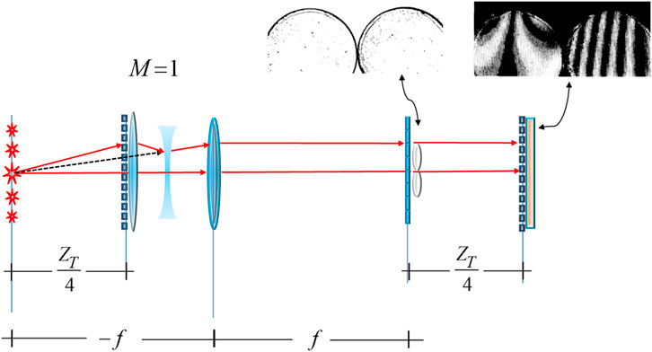
FIGURE 5. Schematics depicting the use of the varifocal system, for generating a no occluding periodic illumination on a sample. At the back focal plane, the no occluding periodic illumination impinges on a pair of transparent disks. At the top of the schematics, we include a photograph of the sample, as well as a photograph of the Talbot interferograms.

We use the complex amplitude distribution, in Eq. (39), for illuminating an object under test. In Figure 5, we show the object under test, which is located at the back focal plane of the optical setup. Then, at a distance Z_T/4 after the back focal plane, we place a second grating for generating Moiré patterns.

The main advantage of this type of illuminations is that it does not generate occluding regions, on the sample under test. For further details, the reader is addressed to the reference (Lohmann, 1988; Leger and Swanson, 1990). In Section 6, we will apply Eq. (39) for describing the propagation of optical short pulses in a dispersive medium.

Regarding the previous results, we recognize that for the same value of z = Z_T/4, but now with M = 2, Eq. (38) becomes

$\psi \left(x,\frac{Z_T}{4}\right)=g\left(x\right).(40)$

Equation (40) indicates the conditon for obtaining a self-image.

Thus, without any longitudinal displacement, we generate an illuminating wave that is structured as the grating itself. Of course, many other possibilities are open by tuning the magnification M.

6 The self-imaging phenomenon in optical fibers

For understanding the formation of spatial self-images inside an optical fiber, it is necessary to consider two conditions. The first condition is to identify the wave functions that represented the Eigen-modes, associated to the propagation inside the guiding media. For the second condition, one needs to express the propagating of an arbitrary wave as a linear superposition of the Eigen-modes. For the self-imaging phenomenon, one requires phase coincidence between the several Eigen-modes. If the condition for phase coincidence is not satisfied, the wave exhibits modal dispersion. Ulrich clearly identified these two conditions (Ulrich, 1975; Ulrich and Ankele, 1975).

For satisfying the first condition, we employ the formal solution of the wave equation inside the guiding media. For clarifying the use of this approach, in what follows, we start by employing the formal solution for a wave that travels in free space. We will note that this treatment leads to the identification of the Bessel beams, as the Eigen-modes of free space propagation. In mathematical terms, for our current discussion, we express Helmholtz equation as follows

$\frac{{\partial }^2}{\partial z^2}\psi \left(x,y,z\right)=-k^2\left[1+k^{-2}\left(\frac{{\partial }^2}{\partial x^2}+\frac{{\partial }^2}{\partial y^2}\right)\right]\psi \left(x,y,z\right).(41)$

The formal solution of Eq. (41) is

$\psi \left(x,y,z\right)=\exp \left[ikz\sqrt{\left(1+k^{-2}\left(\frac{{\partial }^2}{\partial x^2}+\frac{{\partial }^2}{\partial y^2}\right)\right)}\right]\chi \left(x,y\right).(42)$

In Eq. (42), the initial condition is the function χ(x, y) = ψ(x, y, z = 0). Several years ago, for identifying the sufficient and necessary conditions for obtaining self-images, one of us recognized a simple method. The Eigen-modes are obtained by noting that the initial function should satisfy the differential equation

${\nabla }_{\perp }^2\chi \left(x,y\right)=-{\epsilon }^2\chi \left(x,y\right).(43)$

In Eq. (43) the lower-case Greek letter ε represents the Eigenvalue associate to the transversal Laplacian operator, in rectangular coordinates, ${\nabla }_{\perp }^2$ = (∂x² + ∂y²). The Eigenvalue, ε, has dimensions of (1/length). By substituting the left-side of Eq. (43) in Eq. (42), we obtain the mathematical expression for the propagating wave

$\psi \left(x,y,z\right)=\exp \left[ikz\sqrt{\left(1-{\left(\frac{\epsilon }{k}\right)}^2\right)}\right]\chi \left(x,y\right).(44)$

The solution in Eq. (44) is the Eigen-mode. Trivially, Eq. (43) is solved if the initial function is a 2-D plane wave, namely

$\chi \left(x,y\right)=A\exp \left[ik\left(Lx+My\right)\right].(45)$

In Eq. (45) the upper-case letters L an M denote the direction cosines. Then, the Eigen-mode is

$\psi \left(x,y,z\right)=A\exp \left[ikz\sqrt{\left(1-\left(L^2+M^2\right)\right)}\right]\exp \left[ik\left(Lx+My\right)\right].(46)$

Equation (46) represents the propoagation of a tilted plane wave. The obligatory phase coincidence, if you will the modal non-dispersive condition, is the well-known requirement for obtaining self-images. Of course, the above formulation can be repeated for a different coordinate system. Indeed, for cylindrical coordinates, Eq. (42) becomes

$\psi \left(r,\phi ,z\right)=\exp \left[ikz\sqrt{\left(1+k^{-2}\left(\frac{{\partial }^2}{\partial r^2}+\frac{1}{r}\frac{\partial }{\partial r}+\frac{1}{r^2}\frac{{\partial }^2}{\partial {\phi }^2}\right)\right)}\right]\chi \left(r,\phi \right).(47)$

Equation (47) only describes the formal solution. For finding the Eigen-mode, one needs to solve the differential equation

$\left(\frac{{\partial }^2}{\partial r^2}+\frac{1}{r}\frac{\partial }{\partial r}+\frac{1}{r^2}\frac{{\partial }^2}{\partial {\phi }^2}\right)\chi \left(r,\phi \right)=-{\epsilon }^2\chi \left(r,\phi \right).(48)$

It is common in mathematical physics to employ the method of separation of variables, for solving this type of partial differential equation. Hence, we assume that the solution has the form

$\chi \left(r,\phi \right)=R\left(r\right)\exp \left(im\phi \right).(49)$

By placing this function in Eq. (49), we obtain a differential equation for the radial function R(r). That is,

$\left(\frac{d^2}{d{r}^2}+\frac{1}{r}\frac{d}{dr}+{\epsilon }^2-{\left(\frac{m}{r}\right)}^2\right)R\left(r\right)=0.(50)$

By employing the change of variable k r = t, we can rewrite Eq. (50), and its solution, as

$\left(t^2\frac{d^2}{d{t}^2}+t\frac{d}{dt}+t^2-m^2\right)J_m\left(t\right)=0.(51)$

In Eq. (51) the radial function J_m(t) is the Bessel function of the first kind, and integer order m. Therefore, Eq. (52) denotes the Eigen-mode

$\psi \left(r,\phi ,z\right)=A\exp \left[ikz\sqrt{\left(1-m^2\right)}\right]J_m\left(kr\right)\exp \left(im\phi \right).(52)$

For understanding the condition for obtaining self-images, the reader is kindly addressed to Eq. (11) in reference (Lohmann et al., 1983). In that paper, some of us noted that in the frequency domain, the Eigen-modes can be related to the nonparaxial rings, which were used by Montgomery for stating the necessary and sufficient conditions for self-imaging (Montgomery, 1968). It is interesting to note that after 4 years, from the publication of this solution, other researcher rediscovered this solution. The same solution was denoted with the now popular misnomer “diffractionless” beams (Durnin, 1987). Next, we note that the above formulation is indeed also useful for describing wave propagation in a guiding media (Ojeda-Castañeda and Noyola-Isgleas, 1990; Szwaykowski and Ojeda-Castañeda, 1991). Now we consider the following expression for the Helmholtz equation, in cylindrical coordinates,

$\left[{\nabla }_{\perp }^2+\frac{{\partial }^2}{\partial z^2}+k^2{N}^2\left(r\right)\right]\psi \left(r,\phi ,z\right)=0.(53)$

In Eq. (53) we denote the transversal Laplacian operator as in Eq. (54).

${\nabla }_{\perp }^2=\frac{{\partial }^2}{\partial r^2}+\frac{1}{r}\frac{\partial }{\partial r}+\frac{1}{r^2}\frac{{\partial }^2}{\partial {\phi }^2}.(54)$

In Eq. (54), the transversal Laplacian is expressed in polar coordinates. If the employ again the same arguments for finding the Eigen-modes, we need to solve the differential equation

$\left[k^{-2}{\nabla }_{\perp }^2+N^2\left(r\right)\right]R\left(r\right)\exp \left(im\phi \right)=-{\epsilon }^{2}R\left(r\right)\exp \left(im\phi \right).(55)$

Equation (55) is a general differential equation. As in the reference (Ojeda-Castañeda and Noyola-Isgleas, 1990), and in (Okoshi, 1982), we consider the following alpha power, radial refractive index profile. For values of r inside the interval (0, R), the profile is

$N^2\left(r\right)=N_1^2\left[1+A{\left(\frac{r}{R}\right)}^{2\alpha -2}+B{\left(\frac{r}{R}\right)}^{\alpha -2}\right].(56)$

In Eq. (56) the lower case, Greek letter, alpha is a real number. For the values of r, where r > R, the refractive index profile is

$N^2\left(r\right)=N_1^2\left[1+A+B\right]=N_2^2.(57)$

From Eq. (57) we note that if B = 0, then α ≥ 1. And if B ≠ 0, then α ≥ 2. For finding the Eigen-modes, as in Eq. (48), we use the function

$\left[r^2\frac{d^2}{d{r}^2}+r\frac{d}{dr}-m^2+\left(k^2{N}_1-{\epsilon }^2\right)r^2+A{\left(\frac{k{N}_1}{R^{\alpha -1}}\right)}^2{r}^{2\alpha }+B\left(\frac{{\left(k{N}_1\right)}^2}{R^{\alpha -2}}\right)r^{\alpha }\right]R\left(r\right)=0.(58)$

The above differential equation, in Eq. (58), has two expressions that are known in the mathematical physics literature (Bell, 1986). Due to the lengthy derivations, we only discuss one case out of two. For A > 0 and B = 0, according to Bell (Bell, 1986), the differential equation takes the known expression

$\left[r^2\frac{d^2}{d{r}^2}+\left(1-2a\right)r\frac{d}{dr}+\left[\left(a^2-m^2{\gamma }^2\right)+b^2{\gamma }^2{r}^2\right]\right]R\left(r\right)=0.(59)$

By a simple comparison between Eqs (58, 59), we have that

$\alpha =1;a=0;\gamma =1;b=k{N}_1\sqrt{A};R\left(r\right)=J_m\left(\left(k{N}_1\sqrt{A}\right)r\right).(60)$

Thus, by using Eq. (60), for this case, the Eigen-mode is

$\chi \left(r,\phi \right)=c{J}_m\left(\left(k{N}_1\sqrt{A}\right)r\right)\exp \left(im\phi \right).(61)$

In Eq. (61) the lower-case letter “c” denotes an arbitrary constant. To the best of our knowledge, the condition for non modal dispersion is unknown.

7 Self-imaging: statistical aspects

Next, we consider a nonconventional application of the Talbot-Lau effect. We extend our previous descriptions to statistical optics. This description is useful for two specific applications. First, one can evaluate the random movements of a point source as depicted in Figure 6A. Since this type of motion clearly alters the “in-register” condition, one needs a statistical model. Second, for a noncoherent illuminating slit, any geometrical deformations can be considered as the presence of non-aligned, independent point sources as depicted in Figure 6B. For these two applications, it is relevant to comprehend the impact of random locations in an averaged interferogram. To this end, in what follows, we develop the concept of an average optical transfer function (Frieden, 1991). As is discussed in the Supplementary Appendix SC, the average irradiance distribution is

$〈I\left(x\right)〉=\frac{1}{2}+\frac{1}{2}\text{Re}\left\{{\mathrm{\Phi }}_X\left(\frac{1}{d}\right)\exp \left(i2\pi \frac{x}{d}\right)\right\}.(62)$

FIGURE 6

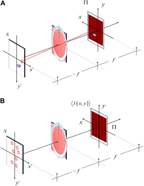
FIGURE 6. Schematics representing a random lateral displacement of a point source, which illuminates with a tilted plane wave a fixed optical grating. In (A) a single point source, at time t = δt. In (B) the several position of the point source at time t. The time average impulse response is denoted as < I (x, y)>.

In Eq. (62), the function Φ_X(μ) denotes the characteristic function of the random process. Its independent variable is the spatial frequency μ. The Fourier transform of Eq. (62) is the average optical transfer function

$〈H\left(\mu \right)〉=\frac{1}{2}\delta \left(\mu \right)+\frac{1}{4}{\mathrm{\Phi }}_X\left(-\frac{1}{d}\right)\delta \left(\mu +\frac{1}{d}\right)+\frac{1}{4}{\mathrm{\Phi }}_X\left(\frac{1}{d}\right)\delta \left(\mu -\frac{1}{d}\right).(63)$

Now, for our numerical simulations, we employ a uniform probability density function that reads

$p_X\left(\zeta \right)=\left(\frac{1}{L}\right)\text{\hspace{0.5em}rect}\left(\frac{\zeta }{L}\right).(64)$

It is worth notincing that in Eq. (63), the spread (of the random positions) is governed by the length, L, of the rectangular window. The Fourier transform of Eq. (64) is the characteristic function, which is

${\mathrm{\Phi }}_X\left(\mu \right)=\text{sinc}\left(L\mu \right).(65)$

The average irradiance distribution is

$〈I\left(x\right)〉=\frac{1}{2}+\frac{1}{2}\text{\hspace{0.5em}sinc}\left(\frac{L}{d}\right)\cos \left(2\pi \frac{x}{d}\right).(66)$

From Eqs (65, 66), we note that the characteristic function impacts on modulation of the detected grating. For visualizing the influence of L on the visibility, in Figure 7 we plot three irradiance distributions associated to three different values of L.

FIGURE 7

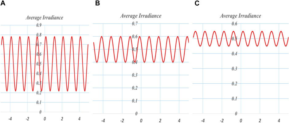
FIGURE 7. Visibility variations caused by the spread of the random locations of a single point source. From (A–C), we assume that the probability density function is uniform, with three different values of L in Eq. (33).

Of course, if the random set of positions obeys a different probability density function, then the visibility will be modulated by a different characteristic function. For example, if the probability density function is Gaussian, with zero mean and with standard deviation equal to σ, the probability density function reads

$p_X\left(\zeta \right)=\exp \left(-\frac{{\zeta }^2}{2{\sigma }^2}\right).(67)$

Please note that Eq. (67) is not normalized. Its characteristic function is

${\mathrm{\Phi }}_X\left(\mu \right)=\exp \left(-2{\left(\pi \sigma \mu \right)}^2\right).(68)$

It is instructive to illustrate the differences, between Eqs (65, 68), by assuming that the characteristic function has the same cut-off, spatial frequency. In Figure 8, we show the probability density functions and their associated characteristic functions.

FIGURE 8

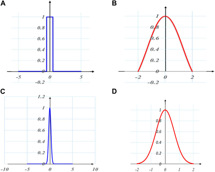
FIGURE 8. Probability density functions and their associated characteristic functions. The cut-off, spatial frequency of the characteristic function is equal to the same value, say, 2 (1/mm). In (A, C) the probability density functions. In (B, D), the characteristic functions. At the top, the uniform distribution. At the bottom, a Gaussian distribution.

For the same cut-off frequency, one expects that for detecting random variations a Gaussian process is more sensitive than a uniform process. In the following section, we extend our previous discussions, by considering the temporal version of the Talbot-Lau effect.

8 Temporal optics: short pulse reconstruction

The Talbot-Lau effect is commonly considered as a purely spatial phenomenon. However, in a renowned paper, Jannson and Jannson noted the similarities between Talbot imaging and the propagation of optical short pulses in a dispersive medium (Jannson and Jannson, 1981). In Figure 9, we show the schematics for our current analysis. We consider the presence of a slow-varying, complex amplitude envelope, χ (t, z), which modulates the continuous wave (CW) coming from a laser. For further details, the reader is kindly addresses to references (Marcuse, 1980; Lohmann and Mendlovic, 1992; Papoulis, 1994; Naulleau and Leith, 1995; Azaña and Muriel, 1999).

FIGURE 9

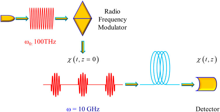
FIGURE 9. Schematics of the setup for analyzing the propagation of the slow-varying complex envelope, along a dispersive medium.

In what follows, we employ the following notation. Along the dispersive medium, the propagation length is z. We consider that a loss-less dispersive medium, which is characterized by a phase-only transfer function. The dispersion function of the medium is β (ω). This function is conveniently expressed as Taylor series expansion, around the angular frequency ω₀. That is,

$\beta \left(\omega \right)={\displaystyle \sum _{n=0}^{\infty }}\frac{1}{n!}{\left(\omega -{\omega }_0\right)}^n{\left.\left[{\left(\frac{d}{d\omega }\right)}^n\beta \left(\omega \right)\right]\right|}_{\omega =\omega {}_0}.(69)$

If in Eq. (69), we consider only the initial three terms, the coefficients are denoted as follows. The first coefficient, Beta sub-zero, is frequency independent and it is consequently ignored. The second coefficient, Beta sub-one, is associated to the group velocity. The third coefficient, Beta sub-two, is known as the first-order, dispersion coefficient. Then, the phase-only transfer function is commonly approximated as

$H\left(\omega \right)=\exp \left(-i\frac{{\beta }_{2}z}{2}{\omega }^2\right).(70)$

Under a convenient analogy, the transfer function in Eq. (70) is like the kernel that is associated to Fresnel diffraction. More on that in what follows. Once that we have the transfer function, we can write the integral transform that describes the time evolution of the slow-varying, complex amplitude

$\chi \left(t,z\right)=\underset{-\infty }{\overset{\infty }{{\displaystyle \int }}}\mathrm{{\rm X}}\left(\omega \right)\exp \left(-i\frac{{\beta }_{2}z}{2}{\omega }^2\right)\exp \left(it\omega \right)d\omega .(71)$

In Eq. (70) the function X(ω) is the Fourier spectrum of the slow-varying, complex amplitude envelope. Equivalently, by remembering that ω = 2 π μ, we can write Eq. (71) as

$\chi \left(t,z\right)=2\pi \underset{-\infty }{\overset{\infty }{{\displaystyle \int }}}G\left(\mu \right)\exp \left(-i2\pi \left(\pi {\beta }_{2}z\right){\mu }^2\right)\exp \left(i2\pi \mu t\right)d\mu .(72)$

In Eq. (72) we change the notation of the functions, G(μ) = X(ω), for incorporating the change of variable, μ = ω/(2 π). Now, it is convenient to remember that a periodic, time signal can be written as the convolution

$g\left(t\right)=u\left(t\right)*{\displaystyle \sum _{m=-\infty }^{\infty }}\delta \left(t-T\right).(73)$

In Eq. (73) the function u(t) denotes the amplitude of the unit pulse, of the periodic time signal. The Fourier spectrum of Eq. (73) is

$G\left(\mu \right)={\displaystyle \sum _{m=-\infty }^{\infty }}U\left(\frac{m}{T}\right)\delta \left(\mu -\frac{m}{T}\right).(74)$

By substituting Eq. (74) in Eq. (72) we obtain the expression that describes the evolution of the slow-varying, complex amplitude envelope

$\chi \left(t,z\right)=2\pi {\displaystyle \sum _{m=-\infty }^{\infty }}U\left(\frac{m}{T}\right)\exp \left(-i2\pi \left(\frac{\pi {\beta }_2}{T^2}z\right)m^2\right)\exp \left(i2\pi \frac{m}{T}t\right).(75)$

By a simple comparison between Eqs. (23, 75), we recognize that there is an analogy between the propagation of slow-varying, complex amplitude envelope and the complex amplitude distribution of a fractional Talbot image. The resemblance can be emphasized by defining the following Talbot distance

$Z_T=\frac{T^2}{\pi {\beta }_2}.(76)$

If one uses the definition in Eq. (76), then Eq. (75) reads

$\chi \left(t,z\right)=2\pi {\displaystyle \sum _{m=-\infty }^{\infty }}U\left(\frac{m}{T}\right)\exp \left(-i2\pi \left(\frac{z}{Z_T}\right)m^2\right)\exp \left(i2\pi \frac{m}{T}t\right).(77)$

From Eqs. (23, 77), we claim that in principle, one can translate the mathematical tools of the spatial Talbot-Lau, to its counterpart in the time domain. For the temporal signals, we can use the mathematical tools that we developed in Section 4, and in the Supplementary Appendix SB. The above-described analogy can help us to understand the possibility of having a Lau effect in the propagation of the slow-varying complex envelope. If you will, one can obtain a noncoherent temporal Talbot effect in the time domain. This idea is depicted in Table 1. For further details, the reader is kindly addressed to the references (Lancis et al., 2006; Torres-Company et al., 2006; Ojeda-Castañeda et al., 2007; Ojeda-Castañeda et al., 2009; Lohmann and Ojeda-Castañeda, 2023).

TABLE 1

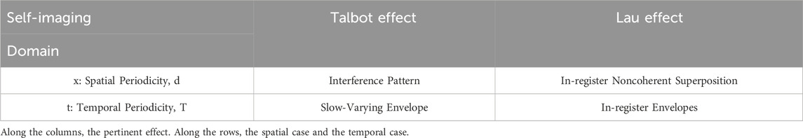
TABLE 1. Table that describes the analogies between the self-imaging phenomena in spatial optics, and in temporal optics.

For emphasizing the analogy under consideration, we discuss the use of the matrix formalism for the temporal case, for N = 2. As in Eq. (35), Section 4, the unit cell changes from its initial function, u(t), to a new function, ψ (t, z). If one uses the formalism in Supplementary Appendix SB, this transformation can be expressed as the matrix product

$\left(\begin{array}{c}{\psi }_0\\ {\psi }_1\end{array}\right)=\left(\begin{array}{cc}{W}_0\left(z\right)& W_1\left(z\right)\\ W_1\left(z\right)& W_0\left(z\right)\end{array}\right)\left(\begin{array}{c}1\\ 0\end{array}\right).(78)$

By substituting the value of the Wn coefficients in Eq. (78) we obtain

$\left(\begin{array}{c}{\psi }_0\\ {\psi }_1\end{array}\right)=\exp \left(-i\pi \frac{z}{Z_T}\right)\left(\begin{array}{cc}\cos \left(\pi \frac{z}{Z_T}\right)& \mathrm{i}\sin \left(\pi \frac{z}{Z_T}\right)\\ \mathrm{i}\sin \left(\pi \frac{z}{Z_T}\right)& \cos \left(\pi \frac{z}{Z_T}\right)\end{array}\right)\left(\begin{array}{c}1\\ 0\end{array}\right).(79)$

Hence, for z = Z_T/4, the matrix product reads

$\left(\begin{array}{c}{\psi }_0\\ {\psi }_1\end{array}\right)=\frac{\sqrt{2}}{2}\exp \left(-i\frac{\pi }{4}\right)\left(\begin{array}{c}1\\ \mathrm{i}\end{array}\right).(80)$

The result in Eq. (80) indicates that the initial unit cell, associated to a binary grating with duty cycle equal to one-half, has been transformed into a unit cell that has two subcells. The new unit cell is a transaparent structure; as is depicted in Figure 10.

FIGURE 10

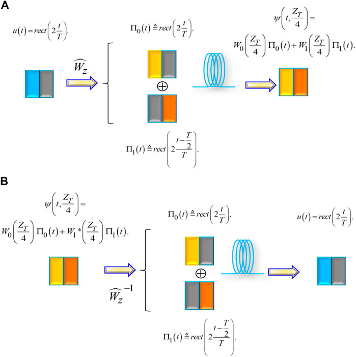
FIGURE 10. Pictorial description on the use of matrix formalism, which illustrates the reversibility on the evolution of the unit cell in a dispersive medium. In (A), the short binary pulse travels a distance equal to one quarter of the Talbot length, z = Z_T/4; and then it becomes a phase-only, short pulse. In (B), the phase-only short pulse travels one quarter of the Talbot length, and it becomes a binary short pulse.

The matrix, at the central part of Eq. (79), has an inverse matrix. Thus, the matrix operation can be reversed. So, we can go back, from a transparent unit cell to amplitude binary cell as is depicted in Figure 10B. It is relevant to note that despite the advantage gained in simplicity, by using the matrix formalism, one cannot describe the ringing effects on the edges of the unit cell. Further details in (Arrizon et al., 1996; Bradburn-Tucker et al., 1999; Ojeda-Castaneda et al., 2015).

9 Conclusion

We have defined an in-register condition. This definition was employed to describe the Lau effect as the noncoherent superposition of independent interferograms. The description consists in adding, in irradiance, several laterally shifted replicas of an initial interferogram. The superposition generates patterns with both high visibility and high light throughput.

We have indicated that for implementing the above procedure, one employs a spatially noncoherent source, which is masked with a periodic set of narrow slits. We have extended this interpretation for increasing the high light throughput of polarization devices, which are commonly employed with a single point source.

For tuning the spatial frequency of the master grating, we have described analytically the method proposed by Luxmoore. And for avoiding the need of any mechanical compensation, we have described the use of a varifocal system, which can magnify the spatial frequency of a master grating. For this type of devices, we have identified the presence of a quadratic phase factor, which can be tuned with the magnification. This result was applied for generating, at a fixed plane, tunable fractions of a Talbot image.

We have further developed the description of the fractional Talbot images, departing from Guigay´s initial proposal. We have expressed the fractional Talbot images as a linear combination of the initial grating. We have applied this formulation for describing a simple array illuminator for Talbot interferometry. The illuminating beam does not generate occluding regions on the sample to be assessed.

The proposed formulation is particularly useful for evaluating the changes of the unit cell, for variable axial locations, z, independently from the number of sub cells. It can mathematically be expressed, in simple terms, by employing a matrix formalism.

We have discussed the use of a differential operator, which solves formally the Helmholtz equation in free space, as well as in guiding media. We have shown that the formal solution helps to obtain the Eigen-modes of free space, and those in guiding media. Simple examples illustrate the benefits of this nonconventional approach.

For proposing sensors that detect random variations, of the position of a point source, we have discussed the use of a time average optical transfer function. And, we have extended our discussion to the reconstruction of sub cells short pulses, which travel along a dispersive medium.

Data availability statement

The original contributions presented in the study are included in the article/Supplementary Material, further inquiries can be directed to the corresponding author.

Author contributions

CG-S: Data curation, Investigation, Software, Validation, Visualization, Writing–review and editing. JO-C: Conceptualization, Formal Analysis, Investigation, Writing–original draft.

Funding

The author(s) declare that no financial support was received for the research, authorship, and/or publication of this article.

Acknowledgments

We express our sincere gratitude to the reviewers, for their valuable and friendly suggestions.

Conflict of interest

The authors declare that the research was conducted in the absence of any commercial or financial relationships that could be construed as a potential conflict of interest.

Publisher’s note

All claims expressed in this article are solely those of the authors and do not necessarily represent those of their affiliated organizations, or those of the publisher, the editors and the reviewers. Any product that may be evaluated in this article, or claim that may be made by its manufacturer, is not guaranteed or endorsed by the publisher.

Supplementary material

The Supplementary Material for this article can be found online at: https://www.frontiersin.org/articles/10.3389/fsens.2023.1328490/full#supplementary-material

References

Andrés, P., Ojeda-Castañeda, J., and Ibarra, J. (1986). Lensless theta decoder. Opt. Commun. 60, 206–210. doi:10.1016/0030-4018(86)90425-6

CrossRef Full Text | Google Scholar

Arrizon, V., Ibarra, J. G., and Ojeda-Castañeda, J. (1996). Matrix formulation of the Fresnel transform of complex transmittance gratings. J. Opt. Soc. Am. A 13, 2414–2422. doi:10.1364/josaa.13.002414

CrossRef Full Text | Google Scholar

Azaña, J., and Muriel, M. A. (1999). Temporal Talbot effect in fiber gratings and its applications. Appl. Opt. 38, 6700–6704. doi:10.1364/ao.38.006700

PubMed Abstract | CrossRef Full Text | Google Scholar

Bachche, S., Nonoguchi, M., Kato, K., Kageyama, M., Koike, T., Kuribayashi, M., et al. (2017). Laboratory-based X-ray phase imaging scanner using Talbot-Lau interferometer for non-destructive testing. Sci. Rep. 7, 6711. doi:10.1038/s41598-017-07032-y

PubMed Abstract | CrossRef Full Text | Google Scholar

Barreiro, J. C., and Ojeda-Castañeda, J. (1993). Degree of coherence: a lensless measuring technique. Opt. Lett. 18, 302–304. doi:10.1364/ol.18.000302

PubMed Abstract | CrossRef Full Text | Google Scholar

Bartelt, H. O., and Jahns, J. (1979). Interferometry based on the Lau effect. Opt. Commun. 30, 268–274. doi:10.1016/0030-4018(79)90351-1

CrossRef Full Text | Google Scholar

Bartelt, H. O., and Li, Y. (1983). Lau interferometry with cross gratings. Opt. Commun. 48, 1–6. doi:10.1016/0030-4018(83)90238-9

CrossRef Full Text | Google Scholar

Bell, W. W. (1986). Special functions for scientists and engineers. London, UK: Van Nostrand, 109.

Google Scholar

Bernardo, L. M., and Soares, O. D. D. (1988). Evaluation of the focal distance of a lens by Talbot interferometry. Appl. Opt. 27, 296–301. doi:10.1364/ao.27.000296

PubMed Abstract | CrossRef Full Text | Google Scholar

Bolognini, N., Ojeda-Castañeda, J., and Sicre, E. E. (1985). Interferometry based on the Lau effect a quasi-ray description. Opt. Acta 3 (2), 409–422. doi:10.1080/713821749

CrossRef Full Text | Google Scholar

Bouffetier, V., Ceurvorst, L., Valdivia, M. P., Dorchies, F., Hulin, S., Goudal, T., et al. (2020). Proof-of-concept Talbot–Lau x-ray interferometry with a high-intensity, high repetition-rate, laser-driven K-alpha source. Appl. Opt. 59, 8380–8387. doi:10.1364/ao.398839

PubMed Abstract | CrossRef Full Text | Google Scholar

Bradburn-Tucker, S., Ojeda-Castañeda, J., and Cathey, W. T. (1999). Matrix description of near field diffraction and the fractional Fourier transform. J. Opt. Soc. Am. A 16, 316–322. doi:10.1364/josaa.16.000316

CrossRef Full Text | Google Scholar

Chang, C. W., and Su, D. C. (1987). Improved collimation testing using Talbot interferometry. Appl. Opt. 26, 4056–4057. doi:10.1364/ao.26.004056

PubMed Abstract | CrossRef Full Text | Google Scholar

Chavel, P., and Strand, T. C. (1984). Range measurement using Talbot diffraction imaging of Gratings. Appl. Opt. 23, 862–871. doi:10.1364/ao.23.000862

PubMed Abstract | CrossRef Full Text | Google Scholar

Chitralekha, S., Avudainayagam, K. V., and Pappu, S. V. (1989). Role of spatial coherence on the rotation sensitivity of Lau fringes: an experimental study. Appl. Opt. 28, 345–349. doi:10.1364/ao.28.000345

PubMed Abstract | CrossRef Full Text | Google Scholar

Cohen-Sabban, Y., and Joyeux, D. (1983). Aberration-free nonparaxial self-imaging. J. Opt. Soc. Am. 73, 707–719. doi:10.1364/josa.73.000707

CrossRef Full Text | Google Scholar

Deng, K., Li, J., and Xie, W. (2020). Modeling the Moiré fringe visibility of Talbot-Lau X-ray grating interferometry for single-frame multi-contrast imaging. Opt. Express 28, 27107–27122. doi:10.1364/oe.400928

PubMed Abstract | CrossRef Full Text | Google Scholar

Dennis, M. R., Zheludev, N. I., and García de Abajo, F. J. (2007). The plasmon Talbot effect. Opt. Exp. 15, 9692–9700. doi:10.1364/oe.15.009692

CrossRef Full Text | Google Scholar

Durnin, J. (1987). Exact solutions for nondiffracting beams I the scalar theory. J. Opt. Soc. Am. A 4, 651–654. doi:10.1364/josaa.4.000651

CrossRef Full Text | Google Scholar

Françon, M., and Mallick, S. (1971). Polarization interferometers: applications and in microscopy and macroscopy. London, U. K.: Wiley-Interscience, 19–28.

Google Scholar

Frieden, B. R. (1991). Probability, statistical optics and data testing. Berlin. Germany: Springer-Verlag, 218–221.

Google Scholar

Gerlich, S., Hacker-Muller, L., Hornberger, K., Stibor, A., Ulbricht, H., Gring, M., et al. (2007). A Kapitza–Dirac–Talbot–Lau interferometer for highly polarizable molecules. Nat. Phys. Lett. 3, 711–715. doi:10.1038/nphys701

CrossRef Full Text | Google Scholar

Gimeno-Gomez, A., Dajkhosh, S. P., Van, C. T. S., Barreiro, J. C., Preza, C., and Saavedra, G. (2023). Management of the axial modulation of the illumination pattern in structured illumination microscopy using an extended illumination source. Opt. Express 31, 36568–36589. doi:10.1364/oe.496518

PubMed Abstract | CrossRef Full Text | Google Scholar

Gómez-Sarabia, C. M., Ledesma-Carrillo, L. M., and Ojeda-Castañeda, J. (2019). Lau-visibility sensor. Opt. Commun. 453, 124320. doi:10.1016/j.optcom.2019.124320

CrossRef Full Text | Google Scholar

Gómez-Sarabia, C. M., and Ojeda-Castañeda, J. (2021). Spectacles with tunable anamorphic ratio, 50. J. of Opt., 453–458.

Google Scholar

Gómez-Sarabia, C. M., and Ojeda-Castañeda, J. (2020a). Hopkins procedure for tunable magnification: surgical spectacles. Appl. Opt. 59, D59–D63. doi:10.1364/ao.385044

PubMed Abstract | CrossRef Full Text | Google Scholar

Gómez-Sarabia, C. M., and Ojeda-Castañeda, J. (2020b). Two-conjugate zoom system: the zero-throw advantage. Appl. Opt. 59, 7099–7102. doi:10.1364/ao.398373

PubMed Abstract | CrossRef Full Text | Google Scholar

Gómez-Sarabia, C. M., and Ojeda-Castañeda, J. (2023a). Tunable Lau effect: optical frequency sweeping. Opt. Commun. 540, 129490. doi:10.1016/j.optcom.2023.129490

CrossRef Full Text | Google Scholar

Gómez-Sarabia, C. M., and Ojeda-Castañeda, J. (2023b). Tunable, nonmechanical, fractional Talbot illuminators. Optics 4, 602–612. doi:10.3390/opt4040045

CrossRef Full Text | Google Scholar

Guigay, J. P. (1971). On Fresnel diffraction by one-dimensional periodic objects, with application to structure determination of phase objects. Opt. Acta 18, 677–682. doi:10.1080/713818491

CrossRef Full Text | Google Scholar

Hall, L. A., Yessenov, M., Sergey, A., Ponomarenko, S. A., and Abouraddy, A. F. (2021). The space–time Talbot effect. Appl. Phys. Lett. Photonics 6, 056105. doi:10.1063/5.0045310

CrossRef Full Text | Google Scholar

Ibarra, J., and Ojeda-Castañeda, J. (1993). Talbot interferometry: a new geometry. Opt. Commun. 96, 294–301. doi:10.1016/0030-4018(93)90278-d

CrossRef Full Text | Google Scholar

Jahns, J., and Lohmann, A. W. (1979). The Lau effect (a diffraction experiment with incoherent illumination). Opt. Commun. 28, 263–267. doi:10.1016/0030-4018(79)90316-x

CrossRef Full Text | Google Scholar

Jannson, T., and Jannson, J. (1981). Temporal self-imaging effect in single-mode fibers. J. Opt. Soc. 71, 1373–1376. doi:10.1364/josa.71.001373

CrossRef Full Text | Google Scholar

Lancis, J., Gómez-Sarabia, C. M., Ojeda-Castaneda, J., Fernández-Pouza, C. R., and Andrés, P. (2006). Temporal Lau effect: noncoherent regeneration of periodic pulse trains. J. Eur. Opt. Soc. 1, 06018. doi:10.2971/jeos.2006.06018

CrossRef Full Text | Google Scholar

Lau, E. (1948). Beugungserscheinungen an doppelrastern (interference phenomenon on double gratings). Ann. Phys. 6, 417.

CrossRef Full Text | Google Scholar

Lee, J., Park, Y., and Chung, S. K. (2019). Multifunctional liquid lens for variable focus and aperture. Sensors Actuators A Phys. 425, 177–184. doi:10.1016/j.sna.2019.01.014

CrossRef Full Text | Google Scholar

Leger, J. R., and Swanson, G. J. (1990). Efficient array illuminator using binary-optics phase plates at fractional-Talbot planes. Opt. Lett. 15, 288–290. doi:10.1364/ol.15.000288

PubMed Abstract | CrossRef Full Text | Google Scholar

Lohmann, A. W. (1988). An array illuminator based on the Talbot effect. Optik 79, 41–45.

Google Scholar

Lohmann, A. W., and Sinzinger, A. W. (1968). Optical information processing. Ilmenau, Germany: Universitaetverlag Technische Universitaet Ilmenau, 184–185.

Google Scholar

Lohmann, A. W., and Mendlovic, D. (1992). Temporal filtering with time lenses. Appl. Opt. 31, 6212–6219. doi:10.1364/ao.31.006212

PubMed Abstract | CrossRef Full Text | Google Scholar

Lohmann, A. W., and Ojeda-Castañeda, J. (2023). Fresnel similarity. Opt. Commun. 205 (249), 397–405. doi:10.1016/j.optcom.2005.01.042

CrossRef Full Text | Google Scholar

Lohmann, A. W., Ojeda-Castañeda, J., and Streibl, N. (1983). Spatial periodicities in coherent and partially coherent fields. Opt. Acta 30, 1259–1266. doi:10.1080/713821349

CrossRef Full Text | Google Scholar

Lohmann, A. W., and Silva, D. E. (1971). An interferometer based on the Talbot effect. Opt. Commun. 2, 413–415. doi:10.1016/0030-4018(71)90055-1

CrossRef Full Text | Google Scholar

Lohmann, A. W., and Silva, D. E. (1972). A Talbot interferometer with circular gratings. Opt. Commun. 4, 326–328. doi:10.1016/0030-4018(72)90069-7

CrossRef Full Text | Google Scholar

Luxmoore, A. (1971). “Optical projection system for the Moiré method of surface strain measurement,” in Optical instruments and techniques. Editor J. H. Dickson (Newcastle upon Tyne, England: Oriel Press), 210–211.

Google Scholar

Marcuse, D. (1980). Pulse distortion in single-mode fibers. Appl. Opt. 19, 1653–1660. doi:10.1364/ao.19.001653

PubMed Abstract | CrossRef Full Text | Google Scholar

Mishra, K., Murade, B., Carree, B., Roghair, I., Oh, J. M., Manukyan, D., et al. (2014). Optofluidic lens with tunable focal length and asphericity. Berlin, Germany: Springer Nature Research.

Google Scholar

Montgomery, W. D. (1968). Algebraic formulation of diffraction applied to self-imaging. J. Opt. Soc. Am. 57, 1112–1124. doi:10.1364/josa.58.001112

CrossRef Full Text | Google Scholar

Morimoto, N., Kimura, K., Shirai, T., Doki, T., Sano, S., Horiba, A., et al. (2020). Talbot–Lau interferometry-based X-ray imaging system, with retractable and rotatable gratings for nondestructive testing. Rev. Sci. Instrum. 91, 023706. doi:10.1063/1.5131306

PubMed Abstract | CrossRef Full Text | Google Scholar

Nakano, Y., and Murata, K. (1985). Talbot interferometry for measuring the focal length of a lens. Appl. Opt. 24, 3162–3166. doi:10.1364/ao.24.003162

PubMed Abstract | CrossRef Full Text | Google Scholar

Naulleau, P., and Leith, E. (1995). Stretch, time lenses, and incoherent time imaging. Appl. Opt. 34, 4119–4128. doi:10.1364/ao.34.004119

PubMed Abstract | CrossRef Full Text | Google Scholar

Neuwirth, T., Backs, A., Gustschin, A., Vogt, S., Pfeiffer, F., Böni, P., et al. (2020). A high visibility Talbot-Lau neutron grating interferometer to investigate stress-induced magnetic degradation in electrical steel. Nat. Sci. Rep. 10, 1764. doi:10.1038/s41598-020-58504-7

PubMed Abstract | CrossRef Full Text | Google Scholar

Nikkhah, H., Hasan, M., and Hall, T. J. (2018). The Talbot effect in a metamaterial. Appl. Phys. A 124, 106. doi:10.1007/s00339-017-1521-1

CrossRef Full Text | Google Scholar

Ojeda-Castañeda, J., Andrés, P., and Barreiro, J. C. (1989a). Abbe-Porter experiment and logic operations. Opt. Commun. 71, 145–150. doi:10.1016/0030-4018(89)90416-1

CrossRef Full Text | Google Scholar

Ojeda-Castañeda, J., Andrés, P., and Ibarra, J. (1998). Lensless theta decoder with high light throughput. Opt. Commun. 67, 256–260. doi:10.1016/0030-4018(88)90145-9

CrossRef Full Text | Google Scholar

Ojeda-Castañeda, J., Andrés, P., and Mendoza-Yero, O. (2009). Tailoring temporal intensities at first- and second-dispersion order. Opt. Memo. Neural Net 18, 260–267. doi:10.3103/s1060992x0904002x

CrossRef Full Text | Google Scholar

Ojeda-Castañeda, J., Barreiro, J. C., and Ibarra, J. (1988). Schardin-Lau interferometer. Opt. Commun. 67, 325–330. doi:10.1016/0030-4018(88)90020-x

CrossRef Full Text | Google Scholar

Ojeda-Castaneda, J., Cristina, M., and Gómez-Sarabia, C. M. (2015). Dispersion of short pulses: Guigay matrix. Phot. Lett. Pol. 7, 17–19. doi:10.4302/plp.2015.1.07

CrossRef Full Text | Google Scholar

Ojeda-Castañeda, J., Ibarra, J., and Barreiro, J. C. (1989b). Noncoherent Talbot effect: coherence theory and applications. Opt. Commun. 71, 151–155. doi:10.1016/0030-4018(89)90417-3

CrossRef Full Text | Google Scholar

Ojeda-Castañeda, J., Lancis, J., Gómez-Sarabia, C. M., Torres-Company, J., and Andrés, P. (2007). Ambiguity function analysis of pulse train propagation: applications to temporal Lau filtering. J. Opt. Soc. Am. A 24, 2268–2273. doi:10.1364/josaa.24.002268

CrossRef Full Text | Google Scholar

Ojeda-Castañeda, J., and Noyola-Isgleas, A. (1990). Nondiffracting wavefields in grin and free-space. Microw. Opt. Technol. Lett. 3, 430–433. doi:10.1002/mop.4650031208

CrossRef Full Text | Google Scholar

Ojeda-Castañeda, J., and Sicre, E. E. (1986). Theta-modulation decoder based on the Lau effect. Opt. Commun. 59, 87–91. doi:10.1016/0030-4018(86)90455-4

CrossRef Full Text | Google Scholar

Okoshi, T. (1982). Optical fibers. New York, NY, USA: Academic Press, 110–287.

Google Scholar

Papoulis, A. (1968). Systems and transforms with applications in optics. New York, U. S. A.: McGraw-Hill, 315–316.

Google Scholar

Papoulis, A. (1994). Pulse compression fiber communications and diffraction: a unified approach. J. Opt. Soc. Am. A 11, 3–13. doi:10.1364/josaa.11.000003

CrossRef Full Text | Google Scholar

Rogers, G. L. (1963). The process of image formation as the re-transformation of the partial coherence pattern of the Object. Phys. Soc. 81, 323–331. doi:10.1088/0370-1328/81/2/314

CrossRef Full Text | Google Scholar

Shurcliff, W. A. (1968). Polarized light: production and use. Cambridge, U. S. A: Harvard University Press, 166–171.

Google Scholar

Silva, D. E. (1971). A simple interferometric method of beam collimation. Appl. Opt. 10, 1980–1982. doi:10.1364/AO.10.1980_1

PubMed Abstract | CrossRef Full Text | Google Scholar

Song, X., Zhang, H., Li, D., Jia, D., and Liu, T. (2020). Electrowetting lens with large aperture and focal length tunability. Berlin, Germany: Springer Nature Research.

Google Scholar

Sriram, K. V., Kothiyal, M. P., and Sirohi, R. S. (1992). Direct determination of focal length by using Talbot interferometry. Appl. Opt. 31, 5984–5987. doi:10.1364/ao.31.005984

PubMed Abstract | CrossRef Full Text | Google Scholar

Su, D. C., and Chang, C. W. (1990). A new technique for measuring the affective focal length of a thick lens or a compound lens. Opt. Commun. 78, 118–122. doi:10.1016/0030-4018(90)90106-4

CrossRef Full Text | Google Scholar

Szwaykowski, P., and Ojeda-Castañeda, J. (1991). Nondiffracting beams and the self-imaging phenomenon. Opt. Commun. 83, 1–4. doi:10.1016/0030-4018(91)90511-b

CrossRef Full Text | Google Scholar

Torres-Company, V., Lancis, J., and Andrés, P. (2006). Unified approach to describe optical pulse generation by propagation of periodically phase-modulated CW laser light. Opt. Express 14, 3171–3180. doi:10.1364/oe.14.003171

PubMed Abstract | CrossRef Full Text | Google Scholar

Ulrich, R. (1975). Image formation by phase coincidences in optical waveguides. Opt. Commun. 13, 259–264. doi:10.1016/0030-4018(75)90095-4

CrossRef Full Text | Google Scholar

Ulrich, R., and Ankele, G. (1975). Self-imaging in homogeneous planar optical waveguides. Appl. Phys. Lett. 27, 337–339. doi:10.1063/1.88467

CrossRef Full Text | Google Scholar

Wen, J., Zhang, Y., and Min Xiao, M. (2013). The Talbot effect: recent advances in classical optics, nonlinear optics, and quantum optics. Adv. Opt. Photonics 5, 83–130. doi:10.1364/aop.5.000083

CrossRef Full Text | Google Scholar

Yokozeki, S., and Suzuki, T. (1971a). Shearing interferometer using the grating as the beam splitter. Appl. Opt. 10, 1575–1580. doi:10.1364/ao.10.001575

PubMed Abstract | CrossRef Full Text | Google Scholar

Yokozeki, S., and Suzuki, T. (1971b). Shearing interferometer using the grating as the beam Splitter. Part 2. Appl. Opt. 10, 1690–1692. doi:10.1364/ao.10.001690

PubMed Abstract | CrossRef Full Text | Google Scholar