Intra-annual and ecoregional differences in physico-chemical data between blackwater and non-blackwater streams in the coastal plains of South Carolina

In the coastal plains of southeastern United States, blackwater streams are relatively common. In South Carolina, many naturally occurring blackwater streams have been identified over decades of water monitoring, particularly when they fail to meet water chemistry expectations originally set based on non-blackwater streams. The South Carolina Department of Environmental Services has collected extensive, often monthly, water chemistry data from both blackwater and non-blackwater systems throughout the Southeastern Plains (SEP) and Middle Atlantic Coastal Plain (MACP) ecoregions. Using these data, we compared seasonal patterns in water chemistry parameters between blackwater and non-blackwater streams. Examining monthly patterns between ecoregions and between site types (blackwater vs. non-blackwater), we observed that pH, total alkalinity, and total phosphorus often differed by both ecoregion and site type. For many parameters, however, differences between ecoregions were stronger than any differences by site type. This work has identified certain parameters that can distinguish blackwater from non-blackwater streams, but it has also shown that blackwater streams, even within one state, are not a monolith. They vary based on the underlying characteristics of the broader region in which they are located. The results of this research are relevant to the entire SEP and MACP ecoregions which jointly include parts of 11 U.S. states. Results are likely relevant to other blackwater rivers and streams in the contiguous United States and other blackwater systems globally, but the extent of relevance will require additional research. From a management perspective, this research has demonstrated that the Omernik Level III ecoregions offer a scale-appropriate means of grouping relatively similar blackwater systems conducive to management. The framework of ecoregions also supports collaborative exchange of information across political boundaries. This includes the exchange of information globally among entities with homologous ecoregions.

1 Introduction

Streams vary temporally with regards to water chemistry (Rodrigues et al., 2018; Soulsby et al., 2001), biota (Ågren et al., 2007; Johnson et al., 2012; Šporka et al., 2006), and physical habitat measures (Dettinger and Diaz, 2000; Garcia-Roger et al., 2011), the exception being those near the equator. This includes streams in the arctic where discharge, temperature and food availability vary with the seasons (Heim et al., 2016). In general, higher latitudes tend to have more extreme or distinct seasons, whereas seasons are less distinct at lower latitudes. And those of the northern and southern mid-latitude regions, between the subtropical and temperate zones, experience what we recognize as the four-season year (Trenberth, 1983). Streams also vary spatially across the landscape. To help account for this variability, frameworks such as ecoregions are used to represent areas where ecosystems are generally similar (Omernik, 1987).

Within the northern mid-latitudes, the coastal plains of the southeastern United States (US) include the Mississippi Delta and Gulf Coast, which includes eastern Texas and the entire state of Florida, as well as the Atlantic seaboard that extends from Florida to New Jersey. Blackwater rivers and streams represent a substantial and diverse aquatic resource within this region (Flotemersch, 2023; Flotemersch et al., 2024; Mallin, 2023; Smock and Gilinsky, 1992). Among the states within this region having substantial blackwater resources is South Carolina, which is classified as having a humid subtropical climate according to the Köppen-Geiger climate classification scheme (Kottek et al., 2006; SCDNR-Climate, 2022), where rainfall is generally concentrated in the warmest months. The more northwestern part of the state tends to have fewer tropical characteristics and typically experiences more days below freezing, more frequent snow, and greater precipitation (SCDNR-Climate, 2022). In contrast, the southeast tends to have more weeks in drought per year and more extreme rainfall events which can lead to extensive flooding. Because of these differences, rivers and streams in South Carolina not only differ seasonally, but those seasonal differences vary across regions of the state.

In the United States, the Clean Water Act (1972) Section 305(b) directs the United States Environmental Protection Agency (USEPA) and states, territories, and other jurisdictions to report on the condition of aquatic resources to assure adequate protection. This is accomplished by the collection of physical, chemical, and biological data from sample sites that are compared to scientifically determined values that represent the bounds of acceptable conditions for different waterbody types. The importance of understanding seasonal differences as they relate to the biotic indices used for condition assessment of rivers and streams has long been recognized (Carlson et al., 2013; Linke et al., 1999; Turak et al., 1999). Most bioassessment and monitoring programs therefore sample within a specified season to control variability, and in most cases, this is the summer low-flow season (Barbour et al., 1999; Flotemersch et al., 2006). This approach has been embraced by many state, tribal (USEPA-BAB, 2023), and federal programs (USEPA-NRSA, 2022; USGS-NAWQA, 2024) in the U.S. Seasonal variability in water quality has been less addressed, as evidenced by numeric standards that typically do not vary across seasons (e.g., SCDHEC-Reg, 2024).

Obviously, there is seasonal variability in analytes like temperature, and with changes in temperature, the capacity of water to hold oxygen changes (Dowling and Wiley, 1986). In South Carolina, precipitation also varies seasonally and influences connectivity of rivers and streams with off-channel habitats, such as pine flatwoods, forest swamps, bottomland hardwoods, and Carolina bays (SCDNR-Wetlands, 2020; Jackson and Scaroni, 2022). In many cases, the water chemistry of these off-channel systems is much different than that of nearby flowing waters, and when connected, can significantly influence the water chemistry of the receiving system. Common water quality analytes influenced by connectivity with wetlands include pH, DOC, and color. Visual changes to the water have led to these being referred to as “blackwater.” Other analytes are often associated with tannin-rich waters (e.g., low DO, low conductivity, and low alkalinity), but values for these analytes may have more to do with the physical setting of the stream than the addition of tannin-rich water (Flotemersch et al., 2024). Nonetheless, the presence of low DO and elevated temperature can be influenced by the presence of tannin-rich waters as the DOC in the water can result in increased water temperatures that ultimately reduce the capacity of the water to hold DO. Elevated levels of DOC can also stimulate increased microbial activity, further lowering DO levels.

The unique water quality of these systems is often problematic for resource managers because natural conditions in blackwater systems can fail to meet existing criteria (Flotemersch, 2023). Problems can also extend beyond commonly measured water quality analytes. For example, the majority of South Carolina blackwater streams assessed for mercury in fish tissue now have fish consumption advisories (SCDHEC-Advisory, 2023). A reasonable first step towards increasing understanding of these dynamic systems is to explore how they compare to non-blackwater systems. Therefore, the objectives of this study were to (1) determine if monthly patterns in water chemistry differed between blackwater and non-blackwater rivers and streams, (2) determine if existing differences were consistent across ecoregions, and (3) provide an overview of water chemistry analytes in the context of blackwater rivers and streams of the study and discuss possible implications for condition assessment (i.e., impaired or not impaired).

While this study uses stream water chemistry data from the state of South Carolina, the results will be directly relevant to other states to the north and south with similar ecosystems. Results are also relevant to other blackwater rivers and streams in the United States and globally as findings contribute to our understanding of similarities and differences among blackwater systems in general. From a management perspective, this research will inform on the utility of ecoregions as a tool for accounting for variability among system types at a scale conducive to management. If ecoregions prove useful, they can be used as a framework for the collaborative exchange of information across political boundaries, including the exchange of information globally among entities with homologous ecoregions. Collectively, this information will improve scientific understanding of blackwater rivers and streams, aid in their identification for condition assessment purposes, and ultimately enhance protection of these unique aquatic resources as prescribed by the Clean Water Act.

2 Methods

2.1 Study area

South Carolina has a diverse climate with average winter air temperatures of about 1–2°C in the mountains to about 12–14°C near the coast, and average summer air temperatures of 19–21°C in the mountains to 23–25°C along the coast, though maximum summer temperatures can exceed 37°C (SCDNR-Climate, 2022). Land cover in the state is roughly 38.5% forested, 15.6% agricultural (i.e., hay/pasture + cultivated crop), 22.0% wetlands, 9.4% developed, 6.3% open water, and 7.5% other land cover types (i.e., herbaceous, shrub/scrub, and barren land) (based on National Land Cover Database (NLCD), Mikhailova et al., 2021). The dominant forest types in the state are mixed mesophytic, oak dominant, northern hardwood, and northern evergreen. The state ranges in elevation from sea level to a high of 1,085 m in the mountains.

A common ecoregional framework used in the United States for environmental management is that developed by Omernik (2004). The boundaries of ecoregions are defined so that each contains a unique set of environmental characteristics such as climate, vegetation, soil type, and geology. This framework provides for ecoregional classifications at four hierarchical levels. At Level I, the continental U.S. is divided into 12 ecoregions, whereas Level IV consist of 967 ecoregions (Omernik and Griffith, 2014; Omernik, 1995, 2004). South Carolina is divided into five distinct Omernik Level III ecoregions (Griffith et al., 2002a) (Figure 1). The following descriptions of these ecoregions borrow heavily from Griffith et al. (2002b). Proceeding from northwest to southeast, these are Blue Ridge (Ecoregion 66), which is part of the Southern Appalachian Mountains, and has high gradient streams. It is part of one of the richest temperate broadleaf forests in the world, with a high diversity of flora and fauna. The Piedmont (Ecoregion 45) is a transitional area between the Blue Ridge and flat coastal plain to the southeast. It is an erosional terrain of moderately dissected irregular plains with some hills. The southeastern border of this ecoregion is largely demarcated by the Fall Line, a physiographic boundary separating it from ecoregions to its southeast. The Southeastern Plains (SEP; Ecoregion 65) consist of irregular plains with broad interstream areas. The Cretaceous or Tertiary-age sands, silts, and clays of the ecoregion contrast geologically with the older metamorphic and igneous rocks of the Piedmont and Blue Ridge. Streams in this area are relatively low-gradient and sandy-bottomed. The Middle Atlantic Coastal Plain (MACP; Ecoregion 63) has a broad transitional boundary with the SCP to the southeast. Poorly drained soils are common, and the region has a mix of coarser and finer textured soils compared to the mostly coarse soils in most of the SCP. Streams in the MACP tend to be sandier than the more southeasterly-located SCP. Lastly, the SCP (Ecoregion 75) consists of mostly flat plains, but it is a heterogeneous region also containing barrier islands, coastal lagoons, marshes, and swampy lowlands along the Atlantic coasts. This ecoregion is generally lower in elevation with less relief and wetter soils than the MACP ecoregion. Streams with mud and muck substrates are common.

Figure 1

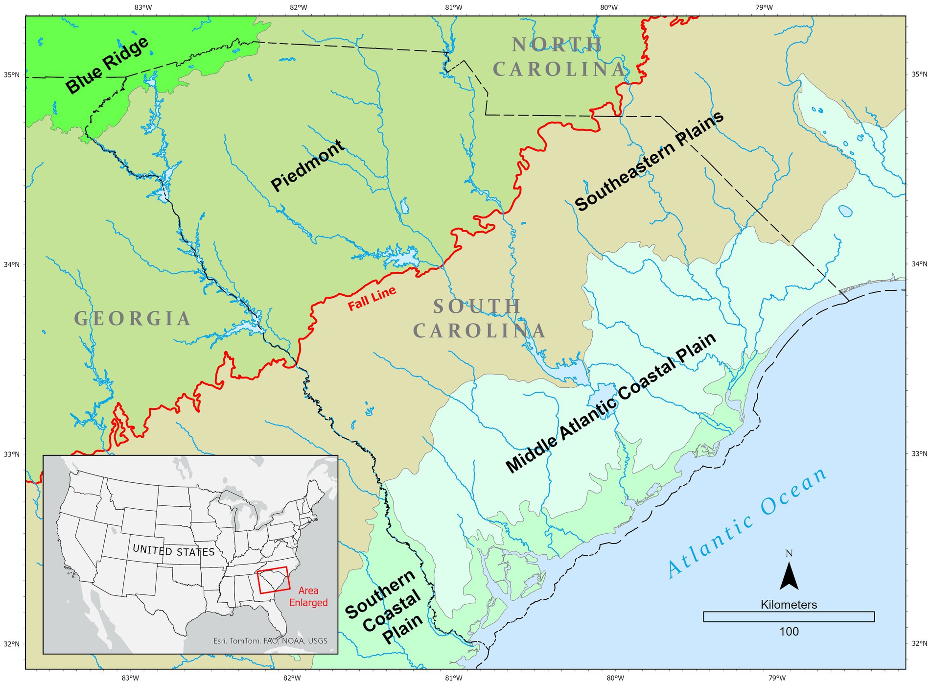
Figure 1. Location of South Carolina within the United States (inset) and in relation to surrounding states. Colored zones within the State represent different Omernik Level III ecoregions. The red line represents the Atlantic Fall Line where the Piedmont and Atlantic Coastal Plain ecoregions meet.

2.2 Dataset

The dataset used in this study contains historic surface water data collected as part of South Carolina Department of Environmental Services’ (SCDES) Ambient Water Quality Monitoring Program (Wilson, 2023). The overall purpose of Ambient Water Quality Monitoring is to provide a system of monitoring activities that produces well-defined data reflecting a variety of water quality conditions (i.e., physical, chemical, biological) in the major water resources of South Carolina, including streams, reservoirs, and saltwaters. Since the early 1970s the program has sampled fixed locations (i.e., base sites) that are generally sampled once per month, year-round. Base sites were chosen to target the most downstream access (pour point) of each of the National Watershed Boundary Dataset 10-digit watershed units in the state, and major waterbody types within watershed units.

A full list of water quality analytes measured as part of the Ambient Water Quality Monitoring Program’s monthly sampling effort is provided in Wilson (2023). Current procedures used for water quality analytes measured in situ and water samples collected for laboratory analysis follow the most current revision and applicable sections of the SCDES Environmental Investigations Standard Operating Procedures and Quality Assurance Manual (SCDES-SOPs, 2024). At their time of collection, all laboratory analyses were performed according to the most current revisions of SCDES Procedures and Quality Control Manual for Chemistry Laboratories and Laboratory Procedures Manual for Environmental Microbiology (SCDES-SOPs, 2024).

It should be noted that, as is the case with any long-term dataset, the equipment and methods used for the collection of in situ measures and processing of laboratory samples over the 50-plus years of the monthly sampling program have evolved. Established quality assurance procedures that have been in place since the inception of the program have functioned to ensure that data has been collected and reported in a uniform manner conducive to providing solid baseline data. Copies of these documents are available from the SCDES’s Environmental Affairs office (www.scdes.gov/environment/).

In South Carolina, water quality standards (SCDHEC-Reg, 2024) Section B.45 defines natural conditions as “water quality conditions unaffected by anthropogenic sources of pollution.” In Section C.9, it also states:

“Because of natural conditions some surface and ground waters may have characteristics outside the standards established by this regulation. Such natural conditions do not constitute a violation of the water quality standards.”

Further, as part of the assessment to determine if sites meet their designated uses (i.e., Clean Water Act §303(d) assessment), sites demonstrating low dissolved oxygen and/or pH relative to numeric standards are examined by experienced SCDES staff to determine if these exceedances are due solely to natural conditions and therefore not true standards exceedances. The state does not have chemical criteria specifically designed to identify blackwater streams. Thus, the following additional characteristics would lead SCDES staff to identify sites as “presumed blackwater”: (1) field observation of staining; (2) significant wetland or swamp drainage adjacent to site; (3) consensus that there were no appreciable potential anthropogenic causes, and the conditions were of natural origin; (4) comparability to nearby sites with past determination of natural conditions. All other sites were presumptively grouped as non-blackwater. It is reasonable to assume that some sites classified as non-blackwater may have displayed dissolved oxygen and/or pH standards exceedances in response to natural conditions, but these exceedances could not be attributed solely to “natural conditions” due to the presence of potential anthropogenic influences. Consequently, the non-blackwater grouping likely contains some sites that are blackwater but have nearby sources of disturbance. Also, some sites that may have blackwater properties yet met dissolved oxygen and/or pH standards would not have been discussed relative to natural conditions and therefore are in the non-blackwater group. Although there is the potential for misclassification based on this subjective approach, we chose to retain the state classification because it represents the best professional judgment of scientists most familiar with the streams and rivers of South Carolina.

The full dataset included data back as far as 1970, but initial inspection of the assembled dataset and knowledge of major changes in methodology for measuring some analytes led to the decision to limit our analysis to data collected after 1998. Examining data from Omernik Level III ecoregions (Omernik, 1987; Omernik and Griffith, 2014), it was noted that nearly all sites designated as “blackwater” were in the Southeastern Plains (SEP) and Middle Atlantic Coastal Plain (MACP) ecoregions (Figure 2; Table 1) in South Carolina. These ecoregions are located southeast of the Fall Line, and northwest of the Southern Coastal Plains ecoregion. Including ecoregions with no or only a few blackwater streams would introduce ecoregional variation in water chemistry that is unrelated to our objective of discerning blackwater from non-blackwater streams. Thus, to control for heterogeneity in the data set (Legendre and Fortin, 1989) due to inclusion of data from ecoregions not containing blackwater systems, only data from SEP and MACP ecoregions were retained for further examination. We then examined data for outliers or extreme values, as well as impossible values or obvious data entry errors that would unduly influence the analysis. An example of an impossible value is a pH of 15, given that the range of possible values is 0–14. Examples of data entry errors were misplaced decimal points that resulted in values one or more orders-of-magnitude out of range and zeros in the dataset entered when values were missing or potentially non-detects. Values that were extreme and likely measured following a storm event were not considered representative of typical flow conditions. To avoid the possibility that these values could drive analysis, we removed 7 individual values from the dataset, which included ammonia + ammonium >25 mg N/L, total Kjeldahl nitrogen >45 mg/L, biochemical oxygen demand >60 mg/L, total nitrogen >600 ug/L, and nitrate + nitrate >400 mg N/L. In total, 7 individual analyte values from 4 stations were removed.

Figure 2

Figure 2. Distribution of blackwater and non-blackwater sampling locations retained for analysis within South Carolina, U.S.A. Triangles indicate sites identified as blackwater and circles indicate sites not identified as blackwater. Red indicates the site was used in both PCA and monthly mean analyses, and yellow indicates the site was dropped from the PCA due to incomplete data.

Table 1

Table 1. Number of blackwater sites by Omernik Level III ecoregion.

In some cases, there were multiple measurements at a station on the same day. To avoid this duplication of data, mean values were calculated by station, analyte, and sampling date. Because the number of years that sampling occurred varied across stations, the median value of each analyte by station, year, and month (when multiple measures were taken within a month) was then calculated for analysis, reducing the dataset to 347,637 data points across 593 sites and 18 analytes. This dataset was filtered to only include station-year-analyte combinations where there were data for at least 9 of 12 months (75% complete for an analyte for a given year), then to only include data from fixed sites having 5 or more years of data. Finally, data were filtered to limit the water quality analytes retained within each ecoregion to those where data were available from a minimum of 5 stations each characterized as blackwater or non-blackwater. That resulted in a dataset for each ecoregion that included only data on analytes from a minimum of 5 blackwater and 5 non-blackwater sites, each having at least 5 years data, and at least 75% complete in any given year. At this point, there were still varying numbers of years of data for a given month and analyte across stations, so the median value was taken for each station-month-analyte combination, resulting in 18,732 data points across 165 sites, 11 analytes (Table 2), and all 12 months, with a maximum of one point per station-analyte-month combination. This was the final dataset used for analysis. The locations of the final set of sites used in each analysis, and their distribution within ecoregions, are shown in Figure 2.

Table 2

Table 2. Physico-chemical and nutrient analytes included in the analysis.

2.3 Data analysis

Descriptive and inferential statistics were used to investigate monthly patterns in water chemistry in blackwater and non-blackwater sites in each ecoregion. All analyses were run using R software (v. 4.3.2; R Core Team, 2023). Ecoregions were analyzed separately and then compared because previous studies have documented that water chemistry can vary significantly by ecoregion (Omernik and Bailey, 1997; Griffith et al., 1999). For mean plots, the median monthly data (i.e., median value by site, month, and analyte) were summarized as the mean and standard error by analyte and month, within each ecoregion and site type (blackwater vs. non-blackwater). A pattern line was added to aid in examination of monthly patterns.

Principal Components Analysis (PCA) of water chemistry data was conducted on each ecoregion to further explore relationships among analytes. The purpose of this analysis was to examine how and whether blackwater and non-blackwater sites grouped when all the variation across multiple visits to sites was incorporated. Descriptive statistics were calculated for each analyte, and analytes with skewness values of <−0.5 or > 0.5 were log10-transformed, and a constant was added if the minimum value was 0. To support visualization of differences and based on the mean plots, which showed that differences among site types and ecoregion were greater during this timeframe, only data from the primary growing season in South Carolina (i.e., April to October) were included. Given that PCA requires complete data for any variables included (no missing values), the analytes retained were selected from the full set of analytes (Table 2), based on the number of non-missing values in the dataset. This maximized the number of observations included in the PCA. The PCAs were then run on a correlation matrix of the data (i.e., variables were centered and scaled) using the princomp function in the stats R package (R Core Team, 2023). Principal components with eigenvalues of at least 1 were retained and plotted to identify patterns in the data. To further examine differences between blackwater and non-blackwaters sites in each ecoregion, box plots of these PCA axes were also generated.

3 Results

Consistent with expected seasonal weather conditions and the associated average air temperatures, water temperatures (TEMP) were lowest in winter, increased in spring, peaked in summer, and declined going into fall and winter (Figure 3A). The general patterns and change in values across months between blackwater and non-blackwater were almost identical. TEMP values themselves were also very similar across ecoregions and for blackwater and non-blackwater.

Figure 3

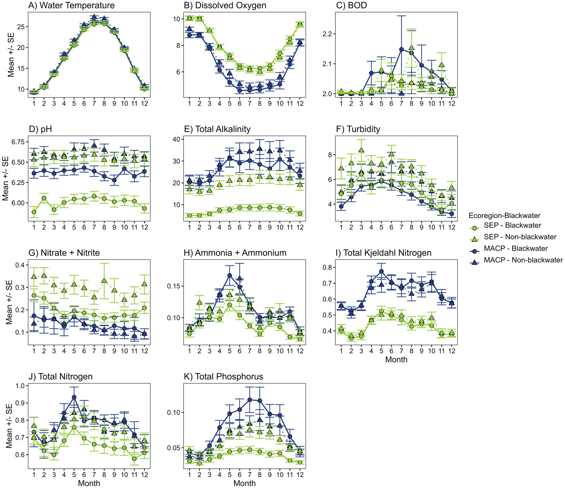
Figure 3. Mean (+/- standard error) line plots of water quality analytes across months of the year. Values are provided for blackwater (circles) and non-blackwater (triangles) sites in the Southeastern Plains (SEP) in green and Middle Atlantic Coastal Plain (MACP) in blue. Numbers on the x-axis correspond to the months of the year. See Table 2 for units.

The general pattern for dissolved oxygen (DO) was consistent among all site types (Figure 3B). Levels were highest in the winter, decreased going into spring, lowest in the summer months, and then increased going into fall and winter. Values were consistently higher in the SEP throughout the year for both blackwater and non-blackwater with minimal differences between blackwater and non-blackwater sites within each ecoregion. Related to DO, values for biochemical oxygen demand (BOD) were more variable. The general pattern for BOD was for levels to be lowest in the winter, increased going into spring and summer, and then decrease going in to fall and winter (Figure 3C). Differences between ecoregions and between blackwater and non-blackwater were mixed.

The general pattern for pH was relatively consistent for all sites with a slight increase in values going into summer and decrease into the fall and winter (Figure 3D). Values for non-blackwater sites in both ecoregions were similar and hovered around a value of 6.6. Values for blackwater sites in the MACP generally ranged between 6.3 and 6.5. Blackwater sites in the SEP were distinctly lower and generally hovered around 6.

The complete full year dataset indicates mean total alkalinity (ALKTOT) was uniformly below 40 mg/L across the study area, and consistently below 10 mg/L in blackwater systems of the SEP (Figure 3E). For all sites, ALKTOT was generally lowest in the winter, increased in the spring, peaked, and leveled off in the summer, and decreased going into fall. The change in values across months, and values in general, were greater for sites in the MACP for both blackwater and non-blackwater sites. Within ecoregions, ALKTOT in non-blackwater sites was clearly greater than that of blackwater systems.

The general pattern for turbidity (TURB) was for values to be lowest in the winter, increasing and peaking in spring, declining through the summer and fall, with declines continuing into winter (Figure 3F). Comparing within the blackwater designation (e.g., SEP blackwater to MACP blackwater), values were higher in the SEP. In both ecoregions, TURB levels were notably lower in blackwater systems than in the non-blackwater systems.

In South Carolina, Total Nitrogen (NTL) is used as a summary measure of nitrogen in water and is calculated as total Kjeldahl nitrogen (TKN) + the combination of nitrate and nitrite (NOx), each of which are measured as nitrogen. TKN is directly measured and represents Total Organic Nitrogen + Ammonia nitrogen (NH₃ + NH₄⁺). Ammonia nitrogen (NH₃-N) as measured represents NH₃ (ammonia) + NH₄⁺ (ammonium). The nutrient measure NOx represents Nitrate (NO₃) + Nitrite (NO₂) as nitrogen. It is used as a stand-alone measure as well as contributing to the calculation of NTL. Total Phosphorus (PTL) is a summary measure of orthophosphate, condensed phosphate, and organic phosphate in water (USEPA-Phosphorus, 2012).

Examining the general pattern of NTL across all sites, values tended to be lowest in late winter and early spring, but then rose sharply in the spring and into early summer (Figure 3J). Through summer, values began to decline before a slight rise in late fall, followed by declining values going into winter. Pattern direction and change in values across months was similar between ecoregions and between blackwater and non-blackwater sites. Between ecoregions, values were greater in the MACP. In the MACP, values are similar between blackwater and non-blackwater sites. In the SEP, NTL tended to be higher in non-blackwater sites.

When examining general patterns for other measures of nitrogen (TKN and NHx), pattern directions parallel those of NTL (Figures 3H–3J). The TKN values were clearly higher than those for NHx. TKN values, between ecoregions, were higher in the MACP than in the SEP. Within ecoregions, TKN values between blackwater and non-blackwater sites were very similar. As for NHx, mean values showed a seasonal peak in the spring and then a decrease through summer and into the fall and winter. Mean values were often higher in the MACP than in the SEP, but not consistently. Within ecoregions, there was not much difference in mean values between blackwater and non-blackwater sites in the MACP, whereas in the SEP, values were consistently higher in non-blackwater sites.

For mean values of NOx, there was not much of a seasonal signal (Figure 3G). Overall, values were higher in the SEP than in the MACP. Within ecoregions, values were higher in the SEP non-blackwater sites than in blackwater sites. Differences between blackwater and non-blackwater sites in the MACP were minimal and inconsistent.

The pattern in PTL across all site types was for lowest levels in the winter, increases in spring, then peak and level off in summer before beginning to decline in the fall and into winter (Figure 3K). The pattern for increasing levels in the spring and summer was much greater in the MACP than in the SEP. Comparing ecoregions, PTL values were higher in the MACP than in the SEP, with values in blackwater systems in the MACP being notably higher than non-blackwater sites. In the SEP, the opposite was true with PTL levels lower in blackwater sites than in non-blackwater sites.

Principal Components Analysis (PCA) of water chemistry data from the April to October growing season was conducted on each ecoregion to explore relationships among analytes. Given that PCA can only be run on sites with complete data, the number of analytes included was reduced to six to maximize the number of sites available for analysis. Analytes retained were pH, TEMP, DO, TURB, NOx, and PTL, each of which had fewer than 10% missing values in the MACP and fewer than 17% missing values in the SEP. For MACP, this reduced the dataset to 32 blackwater and 27 non-blackwater sites. For SEP, the dataset used in PCA included 38 blackwater and 41 non-blackwater sites. Based on the distribution of data by ecoregion, NOx, PTL, and TURB were log10-transformed. Figure 2 distinguishes between sites used in both the mean plots and the PCA and those only in the mean plots.

In the SEP, PC1 and PC2 had eigenvalues of 1.47 and 1.23, respectively, and collectively explained about 61% of the variation (Figure 4A). The higher loadings along PC1 were pH (−0.54), PTL (−0.49), NOx (−0.40), and TURB (−0.49). Along PC2, DO (0.72) and TEMP (−0.47) were the most important analytes. PC1 seemed to be primarily a blackwater vs. non-blackwater axis, whereas PC2 seemed driven by seasonal differences. Box plots of the PCA axes showed a clear distinction between blackwater and non-blackwater along PC1 (Figure 4B), but minimal difference between site types along PC2 (Figure 4C). For both PC1 and PC2, the observed differences between site types were fairly consistent across growing season months (Figures 4B,C). A mild seasonal pattern was evident for both axes.

Figure 4

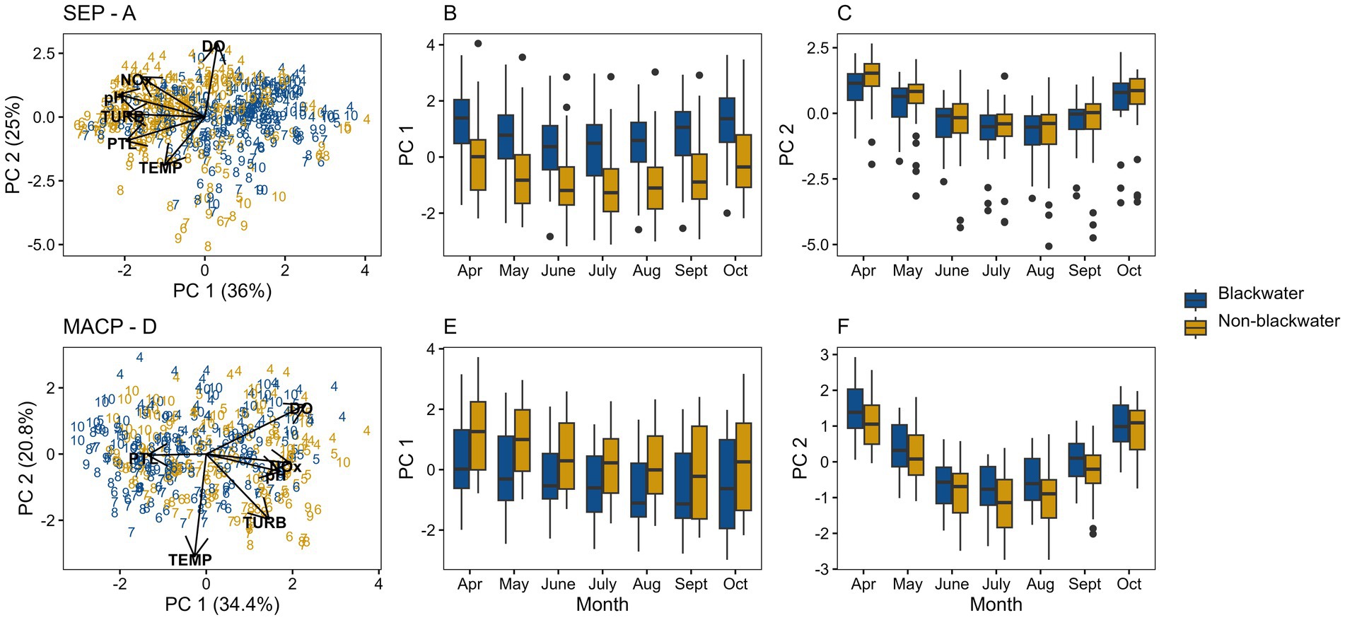
Figure 4. PCA biplots and boxplots of first two principal components for Southeastern Plains (SEP) and Middle Atlantic Coastal Plain (MACP) data. PCA axis 1 (PC 1) and 2 (PC 2) biplots for SEP (A) and MACP (D) represent site-month data points using month number, and axis loadings as vectors. Boxplots in panels (B,E) show PC 1 by month for SEP and MACP, respectively, and in panels (C,F) for PC 2 by month for SEP and MACP, respectively.

In the MACP ecoregion, PC1 and PC2 had eigenvalues of 1.44 and 1.12, respectively, and collectively explained about 55.2% of the variation (Figure 4D). The higher loadings along PC1 were DO (0.57), NOx (0.48), and pH (0.43). Along PC2, TEMP (−0.77) and TURB (−0.49) were the most important analytes. Like the SEP, PC1 seemed to be primarily a blackwater vs. non-blackwater axis and PC2 more driven by seasonal differences for MACP. Box plots of the PC1 were also like those of the SEP, but the separation between blackwater and non-blackwater results were less distinct (Figure 4E) and there was more variation within each month. Observed differences between site types were similar across the growing season. For PC2, differences between blackwater and non-blackwater sites were minimal and consistent for all months of the growing season (Figure 4F). There was a strong seasonal pattern for PC2 for both site types.

4 Discussion

The general patterns for analytes across months, based on mean plot results, were similar between blackwater and non-blackwater sites for both ecoregions. That is, values tended to increase and decrease together across analytes. Between ecoregions, analyte values were notably different for ALKTOT, DO, and all the nutrient measures. Within ecoregion, there were notable differences between blackwater and non-blackwater sites for ALKTOT, pH, and TURB. Differences for these analytes were greater in the SEP than in the MACP, indicating a greater difference between the two stream types in the SEP. Below, the relevance of each analyte to stream condition assessment is discussed, along with an interpretation in the context of blackwaters.

4.1 Physico-chemical Analytes

4.1.1 Alkalinity

ALKTOT is often referred to as the buffering capacity of water in reference to water’s ability to neutralize acids and bases in support of maintaining a relatively stable circumneutral pH (Boyd, 2015; USGS, 2018). It is measured by regulatory organizations because waters with ALKTOT values of 0–50 mg/L have been found to be less biologically productive than those with ALKTOT concentrations of 50–200 mg/L (Moyle, 1946). In surface waters, natural drivers of alkalinity are features of the surrounding landscape such as the geology, soils, and plant activity. A major source of alkalinity in many watersheds is limestone, which contributes carbonates that increase alkalinity (Boyd, 2015; Reimer and Arp, 2011; USGS, 2018). In contrast, areas with igneous rock, such as granite, will have a lower alkalinity (Boyd, 2015; USGS, 2018). Boyd and Walley (1975) summarized this at the soils level by stating lower values were regularly associated with sandy soils while higher values were associated with soils containing available calcium carbonate. This statement is relevant because sandy soils are a common feature of blackwater rivers and streams (Flotemersch et al., 2024) including those of the coastal plains of United States (Smock and Gilinsky, 1992; Flotemersch, 2023; Mallin, 2023).

In the current study, median ALKTOT was uniformly below 40 mg/L across the study area and consistently below 10 mg/L in blackwater sites of the SEP (Figure 3E). Commonly reported values for ALKTOT in fresh waters range from 20 to 200 mg/L (Dikio et al., 2010; Kumar et al., 2010; Ishaq and Khan, 2013; Ustaoğlu et al., 2020). Waters with values less than 10 mg/L are considered to have a very low ALKTOT (Boyd, 2015), and therefore poorly buffered and very susceptible to changes in pH (Dikio et al., 2010).

Values in the SEP ecoregion were lower than those in the more southeasterly-located MACP. Examination of ALKTOT values of the finer-scaled Level IV ecoregions within the SEP and MACP Level III ecoregions (Supplementary Figure 1) showed that ALKTOT values likewise demonstrate a general pattern of increasing ALKTOT proceeding from NW to SE across the study area. These observations concur with those of Omernik and Griffith (1986). Blackwater systems in the most northwesterly-located Level IV ecoregion (Sand Hills, 65c) had the lowest ALKTOT with values hovering around 5 mg/L throughout the year (i.e., very low). Geology in the upper parts of the SEP is composed primarily of Cretaceous-age marine sands and clays, capped in places with Tertiary sands, deposited over the crystalline and metamorphic rocks of the Piedmont (45) to its north, which have a lower ALKTOT (Griffith et al., 2002b).

Moving SE, deposits become younger and transition to more recent Holocene and Pleistocene deposits of the Quaternary (Griffith et al., 2002b) which are not noted for low ALKTOT. Along this same gradient, Carolina Bays and Pocosins decrease in frequency as the frequency of large sluggish rivers and backwaters with ponds, swamps, and oxbow lakes increases. Collectively, these drivers are offered as an explanation for the increasing ALKTOT proceeding from the NW to SE of the study area. These observations are supported by patterns in pH across the study area.

Differences in ALKTOT between blackwater and non-blackwater sites within study ecoregions are likely explained by the extent of connection with wetland habitats. Southern parts of the SEP have high concentrations of Carolina bays and pocosins (Bennett and Nelson, 1991) which are ombrotrophic wetlands perched above the water table and dependent on rainwater. This is significant as rainwater has a low ALKTOT (Weiner and Matthews, 2003) and therefore supports the levels observed at blackwater sites.

4.1.2 pH

Water pH is one of the most important environmental factors influencing species distributions in aquatic habitats. The preferred pH range of individual species differs, but most fall between 6.5 and 8 (USEPA-CADDIS, 2024). In the current study, patterns in pH agreed with what would be expected given the observed ALKTOT values (Figure 3E). This included the slight increase in pH in the summer which aligns with the observed increase in ALKTOT over the same period. Values also largely agree with what would be expected based on observed ALKTOT by site type. Values were lower in the SEP and higher in the MACP. The observed values of pH in response to observed ALKTOT values agrees with the findings of Boyd (2015) who stated that sites with very low (less than 10 mg/L) or low (10–50 mg/L) ALKTOT tended to have a pH value between 5 and 7. Blackwater sites clearly had lower pH values than non-blackwater sites. A reasonable hypothesis for this observation is that blackwaters are receiving significant inputs from wetlands containing low pH dissolved organic carbon (i.e., humic and fulvic acids) into water having low ALKTOT.

4.1.3 Dissolved oxygen and temperature

In fresh waters, DO concentrations fluctuate naturally in response to diurnal (Odum, 1956; Riley and Dodds, 2013) and seasonal changes in TEMP (Dowling and Wiley, 1986; Null et al., 2017; Rajwa-Kuligiewicz et al., 2015), altitude (Jacobsen, 2008; Boyd, 2015), habitat features that facilitate atmospheric aeration (Rajwa-Kuligiewicz et al., 2018), and in response to biological processes (Boyd, 2015). DO levels can also be impacted by a host of anthropogenic activities (USEPA-CADDIS, 2024). Hence, it is routinely monitored by regulatory organizations because aberrant levels can impact both the abiotic and biotic components of aquatic ecosystems (Todd et al., 2009).

Of factors that influence DO levels in streams, seasonal TEMP fluctuations and atmospheric aeration are of special consideration in blackwater systems. In brief, water TEMP influences DO because as TEMP increases, the solubility of oxygen in water decreases (Boyd, 2015). Atmospheric aeration (i.e., opportunities for gaseous exchange) increases with increased turbulence in water. Site characteristics that increase these opportunities include higher flow rates and physical structures like rapids and cascades. Therefore, higher gradient streams generally have higher oxygen levels than lower gradient, slow moving streams (Boyd, 2015; Riđanović et al., 2010).

In the South Carolina dataset, DO values are highest when TEMPs are at their lowest (i.e., winter), and lowest when TEMPs are highest (i.e., summer) (Figure 3A). This agrees with the findings of others examining DO in the Coastal Plains (Ice and Sugden, 2003; Joyce et al., 1985). Comparing DO between the two ecoregions, DO levels are higher in the SEP than in the MACP. These findings agree with those of Smock and Gilinsky (1992) who found that DO levels decreased moving from the upper plains to the lower plains. This can be explained by the gradual decrease in topographic relief from the most NE parts of the SEP to the most SE portions of the MACP. Across this gradient, stream velocities decrease, reducing opportunities for aeration. The occurrence of swamps, marshes, and other backwater habitats also increases (Griffith et al., 2002b). This is significant as it increases opportunities for contributions of low DO water from these habitats to receiving streams. In contrast, little difference is detected between blackwater and non-blackwater in either ecoregion as expected based on the literature (Meyer, 1990, 1992). This suggests that low DO levels reported as a common observation in blackwater rivers and streams are at least in part a function of the physical setting of blackwater rivers and streams (i.e., low gradient). Additional lowering of DO levels likely occurs in blackwaters due to increased heat absorbance of darker waters that increase TEMP and decrease water’s oxygen holding capacity.

4.1.4 Biochemical oxygen demand

Biochemical oxygen demand (BOD) is a measure of the oxygen utilized by bacteria and other microorganisms in the process of decomposition of organic matter under aerobic conditions (USGS, 2018). The rate of this process is also influenced by TEMP (Chapra et al., 2021). High BOD values raise water quality concerns because it can result in low DO levels and impact the flora and fauna of the system (Dogan et al., 2009). Various scales exist for evaluation of BOD values, but in simplest terms, waters with a BOD of 2 mg/L or less would be considered in good condition, 2–10 mg/L—good to somewhat polluted, 10–100 mg/L—somewhat to very polluted, and those over 100 mg/L—very polluted (Maine Environmental Laboratory, 2023; Nasir et al., 2016; Ntengwe, 2006). Considering these criteria, mean BOD values in both ecoregions and in blackwater and non-blackwater systems indicate that systems are in relatively good condition (Figure 3C). However, these are only mean values of data collected over a large time scale.

Despite the generally low mean BOD levels across all sites, there is a tendency for BOD values to be lower in the winter and higher in the summer. This correlates well with increased TEMP and subsequent decreases in DO. Increased microbial activity during the summer months also likely contributes to the observed increase in BOD. While the BOD values in these systems would be considered “good” using currently accepted measures, evaluation guidelines were likely developed based on research conducted on non-blackwater systems. Blackwater systems can often display very low DO levels. In South Carolina, this is primarily in response to the low gradient and low flow velocities common to streams of the Coastal Plains (Mallin et al., 2004). In the current study, DO levels are notably low in MACP streams; slightly more so at blackwater sites. Therefore, even minor increases in anthropogenically-driven BOD (e.g., increased input of effluent, increased nutrient loadings) could result in further declines in DO, pushing the system towards hypoxic conditions stressing benthic and fish communities (Mallin, 2023).

4.1.5 Turbidity

Turbidity is measured in rivers and streams to characterize the relative clarity of the water. Materials that commonly contribute to TURB include clay, silt, suspended inorganic and organic matter, algae, dissolved colored organic compounds, and microscopic organisms (e.g., plankton) (USGS, 2018). In South Carolina, water classification standards call for streams not to exceed 50 NTUs (Nephelometric Turbidity Unit) provided existing uses are maintained (SCDHEC-Reg, 2024). The exception is trout waters, which are rare in the study area and not expected to exceed 10 NTUs. In the current study, values were mostly below 10 NTUs (Figure 3F). Regarding seasonal patterns, increases in the spring are likely due to spring rain events. Decreases thereafter can be explained by reduced rainfall and rain intensity and low-turbidity ground water contributions constituting a greater proportion of the water in the system. Within site type (i.e., blackwater and non-blackwater), TURB levels are higher in the SEP than in the MACP. This can be explained by the gradual decrease in topographic relief across these two ecoregions (see discussion of DO). Water is generally less turbid with decreased flow rates and increased deposition time.

Turbidity values are notably lower in blackwater systems in both ecoregions. Multiple factors likely contribute. First, blackwater systems in the Southeastern Plains are low gradient with minimal flow (Benke and Wallace, 2015; Colvin et al., 2020; Flotemersch, 2023; Mallin et al., 2015; Meyer, 1990; Smock and Gilinsky, 1992), although Flotemersch et al. (2024) presented evidence suggesting that this may not be true of blackwater systems when examined at larger scales. As with DO, lower gradient systems with lower flow rates will have lower TURB (Caruso, 2002; Mallin et al., 2015). Second, blackwater rivers and streams received significant contributions from wetlands, often through subsurface flows (Alexander et al., 2018; Leibowitz et al., 2018). This is evidenced by high levels of DOC and the observation that many blackwater systems seldom flood or dry up in response to the large infiltration capacity of the surrounding landscape (Griffith et al., 2002b). Given that riparian filtration is effective at reducing TURB (Sahu et al., 2019), it would follow that TURB in blackwaters sites would be lower than those at non-blackwater sites.

4.2 Nutrients

Nutrients are regularly measured in aquatic ecosystems as they are one of the most widespread water pollution issues in the United States (USEPA, 2024; USGS, 2018) and globally (UNEP, 2021). Elevated nutrients in a waterbody can stimulate excessive growth of algae and aquatic plants, creating eutrophic conditions that interfere with recreation and the health and diversity of vegetation, insects, fish, and other aquatic organisms. They can also be of risk to human health, especially in the case of elevated levels of nitrates in drinking water (Grout et al., 2023; Ward et al., 2018). Common sources of excess nutrients in rivers and streams include runoff from fertilized lawns and croplands, industrial effluents and domestic sewage discharge, animal waste runoff, atmospheric deposition, and woodland and grassland runoff (UNEP, 2021; USEPA, 2024; USEPA-CADDIS, 2024). These anthropogenic influences could impact observed differences in water quality analytes between blackwater and non-blackwater systems. This is especially true given that research on anthropogenic influences have largely occurred in non-blackwater systems (Flotemersch, 2023; Flotemersch et al., 2024). Consequently, their impact on blackwaters systems is poorly understood. For example, blackwater systems are regularly described in the literature as being nutrient poor and having low DO. What might be considered a minor contribution of nutrients to a non-blackwater system may have more serious consequences to condition in a blackwater system. Despite recognition of these issues, comparisons between systems can be made using published reference values. Reference values published by USEPA as ambient water quality criteria recommendations for SEP and MACP ecoregions (USEPA, 2000a; USEPA, 2000b) are provided to aid interpretation of ecoregional differences in nutrient values where they exist. Reference values were calculated as the lower 25^th percentile of the median of an entire population of data collected across all seasons in each ecoregion.

4.2.1 Nitrogen

For NTL, TKN, and NHx, levels peak in the spring, and again rise in late fall (Figure 3J, I, and H). These patterns are likely in response to the application of fertilizers to agricultural crops during the spring planting season, the fertilization of fall crops, and preparation of fields for spring planting (Almanac, 2024; Wade et al., 2015). The same spring and fall application of nutrients is common in South Carolina for lawns as well (HGIC-CCE, 2019), which likely also contributes to the spring and fall peaks. Between ecoregions, values for the same analytes tend to be higher in the MACP. For NTL and TKN, published reference condition values for NTL and TKN are likewise higher in the MACP (0.71 and 0.37 mg/L, respectively; USEPA, 2000b) than in the SEP (0.69 and 0.30 mg/L, respectively; USEPA, 2000a), so this finding should somewhat be expected. No reference value was available for NHx.

For NOx, values are higher in the SEP than in the MACP, which is reverse of that reported for reference values (USEPA, 2000a; USEPA, 2000b). The SEP does have a higher concentration of permitted livestock operations compared to the MACP (SCDHEC-AAFM, 2019), especially poultry farms (SRAP, 2019) that could be driving this observation. However, if this is true, higher NTL values might be expected as well (Amato et al., 2020). Within the SEP there does not appear to be any obvious explanation for why NOx values are higher in the non-blackwater sites when compared to the blackwater sites.

4.2.2 Total phosphorus

Total phosphorus measures dissolved and particulate sources of phosphorus. In surface waters, it is common for the primary form of phosphorus to be orthophosphate (Watson et al., 2018; Yuan et al., 2015). Orthophosphate is essential for primary production and the principal form of phosphorus available to organisms (Maruo et al., 2016). Excessive levels of phosphorus in freshwaters compromise drinking water procurement, impact biodiversity, and contribute to hypoxia (Sabo et al., 2023, and cited references). In the continental United States, primary drivers of excessive phosphorus levels in streams include annual fertilizer and farm animal manure inputs, and agricultural legacy sources (Sabo et al., 2023; Stackpoole et al., 2019; USGS, 2018). Significant contributions from sewage treatment plants have also been documented (Mallin et al., 2005).

In the current dataset, the pattern across ecoregions and site types is for PTL to be lowest in the winter and highest in the summer (Figure 3K). This again coincides with the primary growing season of agricultural crops in South Carolina, which is therefore a likely contributor to high PTL levels during that timeframe. Between ecoregions, PTL is higher in the MACP than in SEP. This may seem contrary to what might be expected since the southern portion of the SEP (i.e., Atlantic Southern Loam Plains) is a major agricultural area (Griffith et al., 2002b). However, streams draining the southern portion of the SEP quickly enter the northern extent of the MACP, this potentially contributing to the higher values observed therein.

Within the MACP, PTL levels are notably higher in blackwater systems during summer months compared to non-blackwater sites. This could be a direct response to naturally occuring conditions in blackwater rivers and streams. Sediments in rivers and streams are generally considered to be a sink for phosphorus, but this is only true under aerobic conditions. Under anaerobic conditions, orthophosphate (PO₄³⁻) can be mobilized and leached from sediments to the water column (Mulholland, 1992). The probability of this occuring is greater in blackwater rivers and streams which often have naturally occuring low DO levels (Mallin et al., 1999; Mallin et al., 2015; Rudek et al., 1991), some of which may be driven by contributions from wetlands/swamp sediments and decaying organic matter. We found high levels of PTL, which are likely primarily orthophosphate (from above), occurred during the summer months when TEMPs were highest, and DO levels were at their lowest. This would suggest that supplemental contributions of phosphorus to blackwater rivers and streams with naturally occurring low DO levels should be of increased concern.

4.3 PCA

Based on the covariation among analytes observed in the PCAs, the separation between sites classified as blackwater and non-blackwater is greater in the SEP than in the MACP (Figures 4A,D). In the SEP, box plots of PC1 (Figure 4B) show clear separation between blackwater and non-blackwater, but not on PC2 (Figure 4C). Focusing on PC1, we see that the combination of higher pH, TURB, PTL, and NOx all seem to be associated with non-blackwater sites. For the MACP, the separation along PC1 (Figure 4E) is not as clear as in the SEP. In this case, data points with higher pH, NOx, and DO were grouped together at one end of the axis, regardless of stream type. Box plots of the second axis (PC2) in both ecoregions (Figures 4C,F) may account for some additional variation in the data, but it appears to be related to seasonality, rather than blackwater status. Considering these results collectively, the PCA results suggest that differences between sites classified as blackwater and non-blackwater are greater in the SEP than in the MACP.

The greater differences based on PCA observed between blackwater and non-blackwater sites of the SEP are likely in response to a greater range of habitats in that ecoregion. Recall that the SEP is a transitional region between the higher gradients of the Piedmont and the much flatter MACP region. Many of the streams in the SEP originate in the Piedmont and, consequently, represent greater variation in stream habitat than in the MACP. The MACP is more uniformly flat, with swamps, marshes, and estuaries, and this lower level of habitat diversity seems to translate to more consistency in water chemistry between blackwater and non-blackwater streams. The greater range observed for some analytes in line plots of Figure 3 (e.g., pH, ALKTOT, NOx) additionally support the supposition that there is greater habitat diversity in the SEP when compared to the MACP. In other words, the streams in the MACP are more homogenous than those of the SEP.

As a specific example of how differences between the two ecoregions influence water chemistry of blackwaters, and non-blackwater systems as well, Section 4.1.3 discusses DO and TEMP. For both stream types, DO was higher in the SEP than in the MACP. The observed differences were explained by differences in the environmental settings. More specifically, the SEP generally has greater topographic relief than the MACP, and therefore, greater stream water aeration opportunities. While differences in DO between stream types within ecoregions may be minimal, other analytes differ (e.g., BOD and Total Phosphorus; Figures 3C,K). The consequence of these differences, combined with the low DO in the SEP sites, demonstrates how blackwaters can be uniquely impacted when compared to their non-blackwater counterparts.

For management purposes, the PCAs tell us that any distinction between blackwater and non-blackwater streams is consistent across months, meaning that the differences are not strongly seasonal in nature. In the SEP, blackwater and non-blackwater streams are distinctly different. Thus, consideration of separate water quality criteria that are appropriate for blackwater streams may be necessary to fairly assess them in this region. In the MACP, examination of the available parameters revealed strong overlap of blackwater and non-blackwater streams, suggesting that blackwater streams may not require special consideration in this region. However, future research examining additional parameters may indeed identify differences. The lack of differences in the MACP may also be a result of a higher rate of misclassification by SCDES. Improved methods for classification of sites should be considered.

5 Conclusion

The environmental settings and conditions that give rise to blackwater systems are varied. They exist along a multidimensional continuum, although within a given geographic area, a reasonable degree of similarity across systems often exists. In the current study, the general pattern (e.g., increase or decrease) of water quality analyte values across months was similar in the SEP and MACP ecoregions and site types, but the degree of change in values across months differed notably between ecoregions for ALKTOT and PTL. The actual values associated with patterns for analytes were frequently greater in one ecoregion (e.g., ALK, DO, TKN, PTL) or between blackwater and non-blackwater streams (e.g., ALK, pH, PTL, TURB). Where differences occurred, they tended to be most extreme in warmer months. Of analytes we examined, the analytes that best separated blackwater and non-blackwater sites overall in the SEP were pH, ALKTOT, PTL, NOx, and TURB. In the MACP, blackwater and non-blackwater were more clearly separated by PTL, TURB, and pH. In summary, blackwater systems in the two ecoregions exhibited distinct characteristics and therefore cannot be grouped as a single resource type.

Some of the studied blackwater systems exhibited natural conditions that are outside the bounds of what is considered acceptable when compared to the existing condition assessment criteria, i.e., water quality standards adopted by states and Tribes. For example, some blackwater systems had pH and DO levels that were extremely low, both of which can trigger shifts in water quality that impact ecological integrity and human health. Low DO can increase the mobilization of phophorous from sediments. Low pH can increase the availability of undesirable forms of mercury and other metals as well. And both can negatively impact stream biota. Further, the response of these systems to anthropogenic inputs, or the level at which impact occurs, is poorly understood. Therefore, inadequate knowledge of blackwater rivers and streams currently exists to ensure their adequate protection.

While the current research effort utilized stream water chemistry data from South Carolina, the results are relevant to the entire SEP and MACP ecoregions which jointly include parts of 11 U.S. states (i.e., AL, DE, GA, MD, MS, NC, NJ, LA, SC, TN, VA). Results of this study are also likely relevant to other blackwater rivers and streams in the contiguous United States (Flotemersch et al., 2024) and other systems globally, but the extent that this is true remains to be confirmed with additional research. From a management perspective, this research has demonstrated that while blackwater rivers and streams obviously exist along a multidimensional continuum, the scale of Omernik Level III ecoregions offers a means of grouping relatively similar blackwater systems that is conducive to management. Stated differently, Level III ecoregions account for enough variability to be useful, but not so much as to suppress local management utility. The framework of ecoregions also facilitates collaborative exchange of information across political boundaries. This includes the exchange of information globally among entities with homologous ecoregions.

Research needs that would improve understanding and protection of blackwater rivers and streams in South Carolina, the Coastal Plains, and globally, are presented by Flotemersch (2023), and Flotemersch et al. (2024). Findings of the current research effort emphasize that blackwater rivers and streams are not a discrete type of system, but rather an amorphic collection of systems that, in some situations, display unique, if not extreme (e.g., very low pH), natural physico-chemical properties.

Data availability statement

Publicly available datasets were analyzed in this study. These data were originally extracted from the U.S. Water Quality Portal (https://www.waterqualitydata.us/). Data as used in analysis will be provided upon request from authors without undue delay.

Author contributions

KB: Conceptualization, Formal analysis, Investigation, Methodology, Visualization, Writing – original draft, Writing – review & editing. JF: Writing – original draft, Writing – review & editing. HF: Data curation, Writing – review & editing. BR: Conceptualization, Data curation, Visualization, Writing – review & editing. DC: Conceptualization, Writing – review & editing.

Funding

The author(s) declare that no financial support was received for the research, authorship, and/or publication of this article.

Acknowledgments

The U.S. Environmental Protection Agency (USEPA) funded the research described herein, with data preparation support provided by Tetra Tech Inc. under contract number 68HERC22D0026. We thank the associate editor of Frontiers in Water, and the two reviewers for their constructive comments on the manuscript. We also thank Brent Johnson (USEPA/ORD), and Matthew Baumann (SCDES) for their review and comments on this manuscript at various stages of development, and Randy Comeleo (USEPA/ORD) for assistance with revising maps. This article has been reviewed by the Center for Environmental Measurement and Modeling and approved for publication. Mention of trade names or commercial products does not constitute endorsement or recommendation for use by the U.S. Government. The views expressed in this article are those of the authors and do not necessarily reflect the views or policies of the USEPA. All data are publicly available online from the Water Quality Portal (https://www.waterqualitydata.us/).

Conflict of interest

HF was employed by Tetra Tech, Inc.

The remaining authors declare that the research was conducted in the absence of any commercial or financial relationships that could be construed as a potential conflict of interest.

Generative AI statement

The author(s) declare that no Gen AI was used in the creation of this manuscript.

Publisher’s note

All claims expressed in this article are solely those of the authors and do not necessarily represent those of their affiliated organizations, or those of the publisher, the editors and the reviewers. Any product that may be evaluated in this article, or claim that may be made by its manufacturer, is not guaranteed or endorsed by the publisher.

Supplementary material

The Supplementary material for this article can be found online at: https://www.frontiersin.org/articles/10.3389/frwa.2025.1540456/full#supplementary-material

References

Ågren, A., Buffam, I., Jansson, M., and Laudon, H. (2007). Importance of seasonality and small streams for the landscape regulation of dissolved organic carbon export. J. Geophys. Res. Biogeosci. 112:G03003. doi: 10.1029/2006JG000381

Crossref Full Text | Google Scholar

Alexander, L. C., Fritz, K. M., Schofield, K. A., Autrey, B. C., DeMeester, J. E., Golden,, et al. (2018). Featured collection introduction: connectivity of streams and wetlands to downstream waters. J. Am. Water Resour. Assoc. 54, 287–297. doi: 10.1111/1752-1688.12630

Crossref Full Text | Google Scholar

Almanac (2024). 2024 Planting Calendar: When to Plant Vegetables for Places in South Carolina. Available at: https://www.almanac.com/gardening/planting-calendar/SC (Accessed May 02, 2024).

Google Scholar

Amato, H. K., Wong, N. M., Pelc, C., Taylor, K., Price, L. B., Altabet, M., et al. (2020). Effects of concentrated poultry operations and cropland manure application on antibiotic resistant Escherichia coli and nutrient pollution in Chesapeake Bay watersheds. Sci. Total Environ. 735:139401. doi: 10.1016/j.scitotenv.2020.139401

PubMed Abstract | Crossref Full Text | Google Scholar

Barbour, M.T., Gerritsen, J., Snyder, B.D., and Stribling, J.D. (1999). Rapid bioassessment protocols for use in wadeable streams and rivers: periphyton, benthic macroinvertebrates and fish. U.S. Environmental Protection Agency, Office of Water.

Google Scholar

Benke, A. C., and Wallace, B. (2015). High secondary production in a coastal plain river is dominated by snag invertebrates and fuelled mainly by amorphous detritus. Freshw. Biol. 60, 236–255. doi: 10.1111/fwb.12460

Crossref Full Text | Google Scholar

Bennett, S.H., and Nelson, J.B. (1991). Distribution and status of Carolina bays in South Carolina. South Carolina Wildlife and Marine Resources Department. Nongame and Heritage Trust Publications. No. 1. Columbia, SC, USA. Available at: https://www.dnr.sc.gov/wildlife/docs/CarolinaBaysStudy.pdf (Accessed May 28, 2024).

Google Scholar

Boyd, C. E. (2015). Water quality: An introduction. Switzerland: Springer International Publishing.

Google Scholar

Boyd, C.E., and Walley, W.W. (1975). Total alkalinity and hardness of surface waters in Alabama and Mississippi. Agricultural Experiment Station/Auburn University. Bulletin 465. Available at: http://aurora.auburn.edu/bitstream/handle/11200/2397/1647BULL.pdf?sequence=1 (Accessed May 28, 2024).

Google Scholar

Carlson, P. E., Johnson, R. K., and McKie, B. G. (2013). Optimizing stream bioassessment: habitat, season, and the impacts of land use on benthic macroinvertebrates. Hydrobiologia 704, 363–373. doi: 10.1007/s10750-012-1251-5

Crossref Full Text | Google Scholar

Caruso, B. S. (2002). Temporal and spatial patterns of extreme low flows and effects on stream ecosystems in Otago, New Zealand. J. Hydrol. 257, 115–133. doi: 10.1016/S0022-1694(01)00546-7

Crossref Full Text | Google Scholar

Chapra, S. C., Camacho, L. A., and McBride, G. B. (2021). Impact of global warming on dissolved oxygen and BOD assimilative capacity of the world’s rivers: modeling analysis. Water 13:2408. doi: 10.3390/w13172408

Crossref Full Text | Google Scholar

Clean Water Act. (1972). 33 U.S.C. § 1251 et seq. 1972. Available at: https://www.epa.gov/laws-regulations/summary-clean-water-act (Accessed January 21, 2024).

Google Scholar

Colvin, S. A., Helms, B. S., DeVries, D. R., and Feminella, J. W. (2020). Environmental and fish assemblage contrasts in blackwater and clearwater streams. Trans. Am. Fish. Soc. 149, 335–349. doi: 10.1002/tafs.10234

Crossref Full Text | Google Scholar

Dettinger, M. D., and Diaz, H. F. (2000). Global characteristics of stream flow seasonality and variability. J. Hydrometeorol. 1, 289–310. doi: 10.1175/1525-7541(2000)001<0289:GCOSFS>2.0.CO;2

Crossref Full Text | Google Scholar

Dikio, E. D., Mthombeni, L. L., Dikio, C., and Mtunzi, F. (2010). Analysis of fluoride in Vaal River, Sharpeville and Bedworth lakes in the Vaal region of South Africa. Int. J. Appl. Environ. Sci. 5, 691–697.

Google Scholar

Dogan, E., Sengorur, B., and Koklu, R. (2009). Modeling biological oxygen demand of the Melen River in Turkey using an artificial neural network technique. J. Environ. Manag. 90, 1229–1235. doi: 10.1016/j.jenvman.2008.06.004

PubMed Abstract | Crossref Full Text | Google Scholar

Dowling, D.C., and Wiley, M.J. (1986). The effects of dissolved oxygen, temperature, and low stream flow on fishes: A literature review. Illinois Natural History Survey Technical Reports.

Google Scholar

Flotemersch, J. E. (2023). Conservation of Blackwater rivers and streams of the coastal plains of United States: knowledge and research needs. Ambio 52, 665–677. doi: 10.1007/s13280-022-01818-9

PubMed Abstract | Crossref Full Text | Google Scholar

Flotemersch, J. E., Blocksom, K. A., Herlihy, A. T., Kaufmann, P. R., Mitchell, R. M., and Peck, D. V. (2024). Distribution and characteristics of Blackwater rivers and streams of the contiguous United States. Water Resour. Res. 60. doi: 10.1029/2023WR035529

PubMed Abstract | Crossref Full Text | Google Scholar

Flotemersch, J. E., Stribling, J. B., and Paul, M. J. (2006). “Concepts and approaches for the bioassessment of non-wadeable streams and Rivers” in EPA 600-R-06-127. U.S. Environmental Protection Agency (Cincinnati, Ohio).

Google Scholar

Garcia-Roger, E. M., del Mar Sánchez-Montoya, M., Gómez, R., Suárez, M. L., Vidal-Abarca, M. R., Latron, J., et al. (2011). Do seasonal changes in habitat features influence aquatic macroinvertebrate assemblages in perennial versus temporary Mediterranean streams? Aquat. Sci. 73, 567–579. doi: 10.1007/s00027-011-0218-3

Crossref Full Text | Google Scholar

Griffith, G., Omernik, J., and Comstock, J. (2002b). Ecoregions of South Carolina regional descriptions. Corvallis, Oregon, USA: U.S. Environmental Protection Agency.

Google Scholar

Griffith, G.E., Omernik, J.M., Comstock, J.A., Glover, J.B., and Shelburne, V.B. (2002a). Ecoregions of South Carolina. U.S. Environmental Protection Agency, Corvallis, OR (map scale 1:1,500,000). Available at: https://efaidnbmnnnibpcajpcglclefindmkaj/https://upload.wikimedia.org/wikipedia/commons/6/68/South_Carolina_Level_IV_ecoregions.pdf (Accessed February 10, 2025).

Google Scholar

Griffith, G. E., Omernik, J. M., and Woods, A. J. (1999). Ecoregions, watersheds, basins, and HUCs: how state and federal agencies frame water quality. J. Soil Water Conserv. 54, 666–677.

Google Scholar

Grout, L., Chambers, T., Hales, S., Prickett, M., Baker, M. G., and Wilson, N. (2023). The potential human health hazard of nitrates in drinking water: a media discourse analysis in a high-income country. Environ. Health 22:9. doi: 10.1186/s12940-023-00960-5

Crossref Full Text | Google Scholar

Heim, K. C., Wipfli, M. S., Whitman, M. S., Arp, C. D., Adams, J., and Falke, J. A. (2016). Seasonal cues of Arctic grayling movement in a small Arctic stream: the importance of surface water connectivity. Environ. Biol. Fish 99, 49–65. doi: 10.1007/s10641-015-0453-x

Crossref Full Text | Google Scholar

HGIC-CCE. (2019). Fertilizing Lawns. Available at: https://hgic.clemson.edu/factsheet/fertilizing-lawns/ (Accessed May 2, 2024).

Google Scholar

Ice, G., and Sugden, B. (2003). Summer dissolved oxygen concentrations in forested streams of northern Louisiana. South. J. Appl. For. 27, 92–99. doi: 10.1093/sjaf/27.2.92

Crossref Full Text | Google Scholar

Ishaq, F., and Khan, A. (2013). Aquatic biodiversity as an ecological indicator for water quality criteria of river Yamuna in Doon Valley, Uttarakhand, India. World J. Fish Mar. Sci. 5, 322–334. doi: 10.5829/idosi.wjfms.2013.05.03.72126

Crossref Full Text | Google Scholar

Jackson, K.E., and Scaroni, A.E. (2022). An introduction to wetlands of South Carolina. (Clemson, SC: Clemson cooperative extension, land-Grant Press by Clemson extension). LGP 1148. Available at: http://lgpress.clemson.edu/publication/an-introduction-to-wetlands-of-south-carolina (Accessed January 21, 2024).

Google Scholar

Jacobsen, D. (2008). Low oxygen pressure as a driving factor for the altitudinal decline in taxon richness of stream macroinvertebrates. Oecologia 154, 795–807. doi: 10.1007/s00442-007-0877-x

PubMed Abstract | Crossref Full Text | Google Scholar

Johnson, R. C., Carreiro, M. M., Jin, H. S., and Jack, J. D. (2012). Within-year temporal variation and life-cycle seasonality affect stream macroinvertebrate community structure and biotic metrics. Ecol. Indic. 13, 206–214. doi: 10.1016/j.ecolind.2011.06.004

Crossref Full Text | Google Scholar

Joyce, K., Todd, R. L., Asmussen, L. E., and Leonard, R. A. (1985). Dissolved-oxygen, Total organic-carbon and temperature relationships in southeastern United-States coastal-plain watersheds. Agric. Water Manag. 9, 313–324. doi: 10.1016/0378-3774(85)90041-1

Crossref Full Text | Google Scholar

Kottek, M., Grieser, J., Beck, C., Rudolf, B., and Rubel, F. (2006). World map of the Köppen-Geiger climate classification updated. Meteorol. Zeitschrift 15, 259–263. doi: 10.1127/0941-2948/2006/0130

Crossref Full Text | Google Scholar

Kumar, A., Bisht, B. S., Joshi, V. D., Singh, A. K., and Talwar, A. (2010). Physical, chemical and bacteriological study of water from rivers of Uttarakhand. J. Hum. Ecol. 32, 169–173. doi: 10.1080/09709274.2010.11906336

Crossref Full Text | Google Scholar

Legendre, P., and Fortin, M. J. (1989). Spatial pattern and ecological analysis. Vegetatio 80, 107–138. doi: 10.1007/BF00048036

Crossref Full Text | Google Scholar

Leibowitz, S. G., Wigington, P. J. Jr., Schofield, K. A., Alexander, L. C., Vanderhoof, M. K., and Golden, H. E. (2018). Connectivity of streams and wetlands to downstream waters: An integrated systems framework. J. Am. Water Resour. Assoc. 54, 298–322. doi: 10.1111/1752-1688.12631

PubMed Abstract | Crossref Full Text | Google Scholar

Linke, S., Bailey, R. C., and Schwindt, J. (1999). Temporal variability of stream bioassessments using benthic macroinvertebrates. Freshw. Biol. 42, 575–584. doi: 10.1046/j.1365-2427.1999.00492.x

Crossref Full Text | Google Scholar

Maine Environmental Laboratory. (2023). Biochemical oxygen demand (BOD) and CBOD. Available at: https://maineenvironmentallaboratory.com/?p=1175 (Accessed May 1, 2024).

Google Scholar

Mallin, M. A. (2023). “Blackwater streams and rivers” in River Ecology: Science and Management for a Changing World. (United Kingdom: Oxford University Press), 157–168.

Google Scholar

Mallin, M. A., Esham, E. C., Williams, K. E., and Nearhoof, J. E. (1999). Tidal stage variability of fecal coliform and chlorophyll a concentrations in coastal creeks. Mar. Pollut. Bull. 38, 414–422. doi: 10.1016/S0025-326X(99)00024-7

Crossref Full Text | Google Scholar

Mallin, M. A., McIver, M. R., Ensign, S. H., and Cahoon, L. B. (2004). Photosynthetic and heterotrophic impacts of nutrient loading to blackwater streams. Ecol. Appl. 14, 823–838. doi: 10.1890/02-5217

Crossref Full Text | Google Scholar

Mallin, M. A., McIver, M. R., Robuck, A. R., and Dickens, A. K. (2015). Industrial swine and poultry production causes chronic nutrient and fecal microbial stream pollution. Water Air Soil Pollut. 226, 1–13. doi: 10.1007/s11270-015-2669-y

PubMed Abstract | Crossref Full Text | Google Scholar

Mallin, M. A., McIver, M. R., Wells, H. A., Parsons, D. C., and Johnson, V. L. (2005). Reversal of eutrophication following sewage treatment upgrades in the New River estuary, North Carolina. Estuaries 28, 750–760. doi: 10.1007/BF02732912

Crossref Full Text | Google Scholar

Maruo, M., Ishimaru, M., Azumi, Y., Kawasumi, Y., Nagafuchi, O., and Obata, H. (2016). Comparison of soluble reactive phosphorus and orthophosphate concentrations in river waters. Limnology 17, 7–12. doi: 10.1007/s10201-015-0463-6

Crossref Full Text | Google Scholar

Meyer, J. L. (1990). A Blackwater perspective on riverine ecosystems. Bioscience 40, 643–651. doi: 10.2307/1311431

Crossref Full Text | Google Scholar

Meyer, J. L. (1992). “Seasonal patterns of water quality in Blackwater rivers of the coastal plain, southeastern United States” in Water quality in north American River systems. eds. D. Becker and D. A. Neitzel (Columbus, OH: Batelle), 250–275.

Google Scholar

Mikhailova, E. A., Lin, L., Hao, Z., Zurqani, H. A., Post, C. J., Schlautman, M. A., et al. (2021). Land cover change and soil carbon regulating ecosystem services in the state of South Carolina, USA. Earth 2, 674–695. doi: 10.3390/earth2040040

Crossref Full Text | Google Scholar

Moyle, J. B. (1946). Some indices of lake productivity. Trans. Am. Fish. Soc. 76, 322–334.

Google Scholar

Mulholland, P. J. (1992). Regulation of nutrient concentrations in a temperate forest stream: roles of upland, riparian and instream processes. Limnol. Oceanogr. 37, 1512–1526. doi: 10.4319/lo.1992.37.7.1512

Crossref Full Text | Google Scholar

Nasir, A., Nasir, M. S., Shauket, I., Anwar, S., and Ayub, I. (2016). Impact of samanduri drain on water resources of Faisalabad. Adv. Environ. Biol. 10, 155–160.

Google Scholar

Ntengwe, F. W. (2006). Pollutant loads and water quality in streams of heavily populated and industrialised towns. Phys. Chem. Earth Parts A/B/C 31, 832–839. doi: 10.1016/j.pce.2006.08.025

Crossref Full Text | Google Scholar

Null, S. E., Mouzon, N. R., and Elmore, L. R. (2017). Dissolved oxygen, stream temperature, and fish habitat response to environmental water purchases. J. Environ. Manag. 197, 559–570. doi: 10.1016/j.jenvman.2017.04.016

PubMed Abstract | Crossref Full Text | Google Scholar

Odum, H. T. (1956). Primary production in flowing waters 1. Limnol. Oceanogr. 1, 102–117. doi: 10.4319/lo.1956.1.2.0102

Crossref Full Text | Google Scholar

Omernik, J. M. (1987). Ecoregions of the conterminous United States. Ann. Assoc. Am. Geogr. 77, 118–125. doi: 10.1111/j.1467-8306.1987.tb00149.x

Crossref Full Text | Google Scholar

Omernik, J. M. (1995). “Ecoregions: a spatial framework for environmental management” in Biological assessment and criteria: tools for water resource planning and decision making. eds. W. S. Davis and T. P. Simon (Boca Raton, FL.: Lewis Publishers), 49–62.

Google Scholar

Omernik, J. M. (2004). Perspectives on the nature and definition of ecological regions. Environ. Manag. 34, S27–S38. doi: 10.1007/s00267-003-5197-2

Crossref Full Text | Google Scholar

Omernik, J. M., and Bailey, R. G. (1997). Distinguishing between watersheds and ecoregions 1. J. Am. Water Resour. Assoc. 33, 935–949. doi: 10.1111/j.1752-1688.1997.tb04115.x

Crossref Full Text | Google Scholar

Omernik, J. M., and Griffith, G. E. (1986). Total alkalinity of surface waters: a map of the western region. J. Soil Water Conserv. 41, 374–378.

Google Scholar

Omernik, J. M., and Griffith, G. E. (2014). Ecoregions of the conterminous United States: evolution of a hierarchical spatial framework. Environ. Manag. 54, 1249–1266. doi: 10.1007/s00267-014-0364-1

PubMed Abstract | Crossref Full Text | Google Scholar

R Core Team. (2023). R: A language and environment for statistical computing. R Foundation for Statistical Computing, Vienna, Austria. Available at: https://www.R-project.org/ (Accessed June 14, 2024).

Google Scholar

Rajwa-Kuligiewicz, A., Bialik, R. J., and Rowiński, P. M. (2015). Dissolved oxygen and water temperature dynamics in lowland rivers over various timescales. J. Hydrol. Hydromech. 63, 353–363. doi: 10.1515/johh-2015-0041

Crossref Full Text | Google Scholar

Rajwa-Kuligiewicz, A., Plesiński, K., Russell Manson, J., Radecki-Pawlik, A., and Rowiński, P. M. (2018). “Spatial distribution of dissolved oxygen at rapid hydraulic structures as an Indicator of local-scale processes” in Free surface flows and transport processes. eds. M. Kalinowska, M. Mrokowska, and P. Rowiński (Cham: Springer International Publishing), 377–387.

Google Scholar

Reimer, A., and Arp, G. (2011). “Alkalinity” in Encyclopedia of Geobiology. eds. J. Reitner and V. Thiel (Dordrecht: Springer Netherlands), 20–24.

Google Scholar

Riđanović, L., Riđanović, S., Jurica, D., and Spasojević, P. (2010). Evaluation of water temperature and dissolved oxygen regimes in river Neretva. BALWOIS 2010 fourth international conference. Ohrid: Republic of Macedonia.

Google Scholar

Riley, A. J., and Dodds, W. K. (2013). Whole-stream metabolism: strategies for measuring and modeling diel trends of dissolved oxygen. Freshwater Sci. 32, 56–69. doi: 10.1899/12-058.1

Crossref Full Text | Google Scholar

Rodrigues, V., Estrany, J., Ranzini, M., de Cicco, V., Martín-Benito, J. M. T., Hedo, J., et al. (2018). Effects of land use and seasonality on stream water quality in a small tropical catchment: the headwater of Córrego Água Limpa, São Paulo (Brazil). Sci. Total Environ. 622-623, 1553–1561. doi: 10.1016/j.scitotenv.2017.10.028

Crossref Full Text | Google Scholar

Rudek, J., Paerl, H. W., Mallin, M. A., and Bates, P. W. (1991). Seasonal and hydrological control of phytoplankton nutrient limitation in the Neuse River estuary, North Carolina. Mar. Ecol. Prog. Ser. 75, 133–142. doi: 10.3354/meps075133

Crossref Full Text | Google Scholar

Sabo, R. D., Pickard, B., Lin, J., Washington, B., Clark, C. M., Compton, J. E., et al. (2023). Comparing drivers of spatial variability in U.S. lake and stream phosphorus concentrations. J. Geophys. Res. Biogeosci. 128:e2022JG007227. doi: 10.1029/2022JG007227

Crossref Full Text | Google Scholar

Sahu, R. L., Dash, R. R., Pradhan, P. K., and Das, P. (2019). Effect of hydrogeological factors on removal of turbidity during river bank filtration: laboratory and field studies. Groundw. Sustain. Dev. 9:100229. doi: 10.1016/j.gsd.2019.100229

Crossref Full Text | Google Scholar

SCDES-SOPs. (2024). Standard operating procedures. Available from SCDHEC Bureau of Environmental Health Services and/or SCDHEC Bureau of Water. Available at: https://scdhec.gov (Accessed January 24, 2024).

Google Scholar

SCDHEC-AAFM (2019). Available at: https://scdhec.gov/environment/your-water-coast/agricultural-runoff-waste/agricultural-animals-facility-maps (Accessed May 7, 2024).

Google Scholar

SCDHEC-Advisory. (2023). South Carolina fish consumption advisory. Available at: https://gis.dhec.sc.gov/gisportal/apps/webappviewer/index.html?id=c71943bc743b4ca196e0ef0406b1d7ab (Accessed January 23, 2024).

Google Scholar

SCDHEC-Reg. (2024). Regulation 61–68, water classifications and standards. Available at: https://scdhec.gov/sites/default/files/Library/Regulations/R.61-68.pdf (Accessed January 19, 2024).

Google Scholar

SCDNR-Climate. (2022). Overview of South Carolina’s climate and hazards. South Carolina state climatology office, land, water, and conservation division, South Carolina Department of Natural Resources Available at: https://www.dnr.sc.gov/climate/sco/Publications/SCClimateOverview.pdf. (Accessed January 19, 2024).

Google Scholar

SCDNR-Wetlands (2020). Wetlands. Overview. Available at: https://www.dnr.sc.gov/wildlife/wetlands/ (Accessed January 21, 2024).

Google Scholar

Smock, L. A., and Gilinsky, E. (1992). “Coastal plain blackwater streams” in Biodiversity of the southeastern United States: aquatic communities. eds. C. T. Hackney, S. M. Adams, and W. H. Martin (New York: Wiley), 271–313.

Google Scholar

Soulsby, C., Malcolm, R., Gibbins, C., and Dilks, C. (2001). Seasonality, water quality trends and biological responses in four streams in the Cairngorm Mountains, Scotland. Hydrol. Earth Syst. Sci. 5, 433–450. doi: 10.5194/hess-5-433-2001

Crossref Full Text | Google Scholar

Šporka, F., Vlek, H. E., Bulankova, E., and Krno, I. J. (2006). “Influence of seasonal variation on bioassessment of streams using macroinvertebrates” in The ecological status of European rivers: Evaluation and intercalibration of assessment methods. eds. M. T. Furse, D. Hering, K. Brabec, A. Buffagni, L. Sandin, and P. F. M. Verdonschot (Dordrecht: Springer Netherlands), 543–555.

Google Scholar

SRAP. (2019). Guide to confronting concentrated animal feeding operations in South Carolina. Available at: https://sraproject.org (Accessed May 2, 2024).

Google Scholar

Stackpoole, S. M., Stets, E. G., and Sprague, L. A. (2019). Variable impacts of contemporary versus legacy agricultural phosphorus on U.S. river water quality. Proc. Natl. Acad. Sci. 116, 20562–20567. doi: 10.1073/pnas.1903226116

PubMed Abstract | Crossref Full Text | Google Scholar

Todd, M. J., Vellidis, G., Lowrance, R. R., and Pringle, C. M. (2009). High sediment oxygen demand within an instream swamp in southern Georgia: implications for low dissolved oxygen levels in coastal Blackwater streams. J. Am. Water Resour. Assoc. 45, 1493–1507. doi: 10.1111/j.1752-1688.2009.00380.x

Crossref Full Text | Google Scholar

Trenberth, K. E. (1983). What are the seasons? Bull. Am. Meteorol. Soc. 64, 1276–1282. doi: 10.1175/1520-0477(1983)064<1276:WATS>2.0.CO;2

Crossref Full Text | Google Scholar

Turak, E., Flack, L. K., Norris, R. H., Simpson, J., and Waddell, N. (1999). Assessment of river condition at a large spatial scale using predictive models. Freshw. Biol. 41, 283–298. doi: 10.1046/j.1365-2427.1999.00431.x

Crossref Full Text | Google Scholar

UNEP. (2021). World water quality assessment: Ecosystems and water quality Available at: https://www.unep.org/interactives/wwqa/technical-highlights/ecosystems-and-water-quality (Accessed May 2, 2024).

Google Scholar

USEPA. (2000a). Ambient water quality criteria recommendations: Rivers and streams in nutrient ecoregion IX. EPA/822/B/00/019. Available at: https://www.epa.gov/sites/default/files/documents/rivers9.pdf (Accessed May 28, 2024).

Google Scholar

USEPA. (2000b). Ambient water quality criteria recommendations: rivers and streams in nutrient ecoregion XIV. EPA/822/B/00/022. Available at: https://www.epa.gov/sites/default/files/documents/rivers14.pdf (Accessed May 28, 2024).

Google Scholar

USEPA. (2024). Nutrient Pollution. Available at: https://www.epa.gov/nutrientpollution (Accessed May 2, 2024).

Google Scholar

USEPA-BAB. (2023). Available at: https://www.epa.gov/wqc/information-bioassessment-and-biocriteria-programs-streams-and-wadeable-rivers (Accessed January 19, 2024).

Google Scholar

USEPA-CADDIS. (2024). Nutrients. Available at: https://www.epa.gov/caddis/nutrients (Accessed May 2, 2024).

Google Scholar

USEPA-NRSA (2022). Available at: https://www.epa.gov/national-aquatic-resource-surveys/nrsa (Accessed January 19, 2024).

Google Scholar

USEPA-Phosphorus. (2012). Phosphorus. Available at: https://archive.epa.gov/water/archive/web/html/vms56.html (Accessed May 2, 2024).

Google Scholar

USGS. (2018). Water science school. Available at: https://www.usgs.gov/special-topics/water-science-school/science/ (Accessed May 2, 2024).

Google Scholar

USGS-NAWQA. (2024). Method, sampling, and analytical protocols. Available at: https://water.usgs.gov/nawqa/protocols/methodprotocols.html (Accessed 19 January 2024).

Google Scholar

Ustaoğlu, F., Tepe, Y., and Taş, B. (2020). Assessment of stream quality and health risk in a subtropical Turkey river system: a combined approach using statistical analysis and water quality index. Ecol. Indic. 113:105815. doi: 10.1016/j.ecolind.2019.105815

Crossref Full Text | Google Scholar

Wade, T., Claassen, R., and Wallander, S. (2015). Conservation-practice adoption rates vary widely by crop and region, EIB-147, U.S. Department of Agriculture, Economic Research Service, December 2015.

Google Scholar

Ward, M. H., Jones, R. R., Brender, J. D., De Kok, T. M., Weyer, P. J., Nolan, B. T., et al. (2018). Drinking water nitrate and human health: an updated review. Int. J. Environ. Res. Public Health 15:1557. doi: 10.3390/ijerph15071557

PubMed Abstract | Crossref Full Text | Google Scholar

Watson, S. J., Cade-Menun, B. J., Needoba, J. A., and Peterson, T. D. (2018). Phosphorus forms in sediments of a river-dominated estuary. Front. Mar. Sci. 5:302. doi: 10.3389/fmars.2018.00302

Crossref Full Text | Google Scholar

Weiner, R., and Matthews, R. (2003). Environmental engineering. 4th Edn. Burlington, MA: Butterworth-Heinemann.

Google Scholar

Wilson, K. (2023). State of South Carolina monitoring strategy for calendar year 2022. South Carolina State Documents Depository. Technical Report No. 001–2023. Available at: https://scdhec.gov/sites/default/files/media/document/SC%20State%20Monitoring%20Strategy%202023_Updated%2020Jan_signed.pdf (Accessed January 17, 2023).

Google Scholar

Yuan, H. Z., Pan, W., Ren, L. J., Liu, E. F., Shen, J., Geng, Q. F., et al. (2015). Species and biogeochemical cycles of organic phosphorus in sediments from a river with different aquatic plants located in Huaihe river watershed, China. Int. J. Phytoremed. 17, 215–221. doi: 10.1080/15226514.2013.876969

Crossref Full Text | Google Scholar