Integrating groundwater pumping data with regression-enhanced random forest models to improve groundwater monitoring and management in a coastal region

Groundwater is essential for sustaining human life and ecosystems as a freshwater resource. However, intensive groundwater pumping (GWP) can deplete groundwater levels, and exacerbate issues such as sea-level rise and saltwater intrusion in coastal areas, further affecting the availability and accessibility of groundwater. To address these challenges, accurate monitoring and modeling of water table depth (WTD), a key indicator of groundwater storage, is useful for sustainable groundwater management. This work studies the implementation of a regression-enhanced random forest (RERF) model to predict WTD anomalies with pumping as a major input for New Jersey, a coastal state in the United States. The predicted WTD anomalies align well with observations, with a test Nash-Sutcliffe Efficiency (NSE) of 0.49, a test Pearson correlation coefficient (r) of 0.72, and a test root-squared mean error (RMSE) of 1.61 m. Based on a permutation feature importance, the most important input variables in the model for predicting WTD anomalies were long-term mean WTD, precipitation minus evapotranspiration (PME), and GWP. Using the trained RERF model, we generated 90 m spatial resolution WTD anomaly maps for New Jersey for January and July 2015, showing areas of increasing and decreasing WTD. We then inverted the RERF model to predict GWP using WTD anomalies, land cover, and a cross metric as additional inputs. This approach was less effective, yielding a test NSE of 0.40, a test r of 0.65, and a test RMSE of 15.44 million liters/month. A permutation feature importance revealed the most important input variables to be PME, long-term mean WTD, and topographic slope. Again we generated 90 m GWP maps for New Jersey for January and July 2015, offering finer resolution than the previous maps at the subwatershed level. Focusing on New Jersey, the study provides insights into the relationship between WTD anomalies and its critical input variables including GWP in coastal areas. Moreover, significant gaps in WTD observations persist in New Jersey, highlighting the need for comprehensive monitoring efforts. Thus, by employing ML techniques and leveraging available data, this study contributes to improving groundwater management practices and informing future decision-making.

1 Introduction

Groundwater is a critical natural resource for sustaining human life and ecosystems as a freshwater source. Shallow groundwater can impact land surface dynamics in various ways, especially during dry periods, by supplying baseflow to rivers and lakes, sustaining aquatic ecosystems, and providing root-zone soil water, which helps plants with photosynthetic production (Scanlon et al., 2023). Groundwater accessibility and availability are typically studied through water table depth (WTD), the distance between the upper surface of saturated aquifers, and the surface of the ground (Kollet and Maxwell, 2008). Thus, monitoring and recording WTD is crucial for sustainable groundwater management.

Groundwater depletion, referred to as the long-term increase in WTD, is a serious issue worldwide (Konikow and Kendy, 2005; Rodell et al., 2018; Rodell and Reager, 2023). In addition to climate change (Green et al., 2011), unsustainable groundwater pumping (GWP) is a major cause of groundwater depletion (de Graaf et al., 2019; Jasechko et al., 2024). In coastal areas, intensive GWP contributes to sea level rise, ultimately resulting in groundwater inundation and saltwater intrusion (Jasechko et al., 2020; Han and Currell, 2022; Peters et al., 2022; van Engelen et al., 2022; Kuang et al., 2024). Therefore, it is important to improve the regulation of GWP. However, the biggest challenge to effectively managing and mitigating groundwater depletion is the limited availability of groundwater measurements including WTD and GWP records. Insufficient monitoring of groundwater is a problem even in developed countries because of little funding and investments in the equipment installations and maintenance. The way groundwater monitoring is fragmented also leads to inconsistent data collection methods and difficulties in sharing data between groups (Taylor and Alley, 2001).

Machine Learning (ML) approaches have recently emerged as an effective method for groundwater resource modeling (Tao et al., 2022). The appeal of ML models lies in their ability to rapidly predict groundwater data (e.g., WTD) after proper training, potentially reducing the need for an in-depth understanding of the underlying topographical and hydro-geophysical parameters (Ahmadi et al., 2022; Tao et al., 2022). Due to their comparable accuracy to physically-based numerical methods and much lower computational cost, ML models have become a common alternative to traditional physically-based hydrological models, especially for fast decision making. ML have been successfully applied to karst spring discharge simulation (De Filippi et al., 2024; Pölz et al., 2024), groundwater level forecasting (Boo et al., 2024), groundwater quality estimation (Che Nordin et al., 2021), as well as groundwater salinization modeling (Sarkar et al., 2024). As a popular use of ML in groundwater resource modeling, past studies have used a multitude of ML techniques for predicting groundwater levels or WTD, ranging from deep neural networks such as Long Short-Term Memory networks (Ma et al., 2021, 2022; Vu et al., 2021) and convolutional neural networks (Wunsch et al., 2022), simple feedforward neural networks (also called multilayer perceptrons) (Sun, 2013; Gholami et al., 2015), to tree-based ensemble learning methods such as random forest (RF) models (Sahoo et al., 2018). Various datasets have been utilized, including simulation results, in-situ measurements, and remotely sensed data. Nevertheless, GWP has barely been considered in ML models due to the lack of long-term records.

While many studies have proven the effectiveness of using neural networks for WTD or groundwater level prediction, tree-based ensemble learning methods present several benefits over them when training data is limited. In comparison with neural networks, tree-based models have a relatively simple architecture with a smaller number of hyperparameters to tune, thus requiring less training data (Ma et al., 2024). In addition, tree-based models do not need excessive input manipulation (e.g., data normalization), so comparatively little time is invested in input data preprocessing, one of the most important and time-consuming steps in ML model construction. Above all, tree-based models provide feature importance, allowing for an easier understanding of their decision-making process (Breiman, 2001; Müller and Guido, 2017). Yet, traditional tree-based models face the extrapolation issue, and they cannot detect trends to infer values beyond the training set (Zhang et al., 2019). As a result, they are less frequently applied in regression problems such as WTD or groundwater level prediction.

Here we used a variant of the RF model, a regression-enhanced random forest (RERF) model, to predict WTD anomalies (i.e., a variable showing temporal variations in WTD) and GWP in New Jersey, a coastal state in the United States with 30-year pumping records available at the 14-digit hydrologic unit (HUC14) level. Even in New Jersey, we did not have access to records for pumping rates and therefore used monthly aggregated groundwater withdrawal data to represent GWP. The HUC14s are subwatersheds delineated by the United States Geological Survey (USGS) based on surface hydrologic features, which are uniquely identified by a 14-digit number. The RERF model retains the advantages of tree-based models mentioned above and resolves the extrapolation issue, enabling it to predict for unseen inputs (Zhang et al., 2019). Hence, the model can provide spatially continuous predictions despite unmonitored regions lacking observations (Rosecrans et al., 2022). It also avoids biased results that ML regression often produces, where small values are overestimated and large values are underestimated (Belitz and Stackelberg, 2021). Our constructed RERF model is used to predict WTD anomalies in New Jersey with GWP as a major input and then inverted to estimate GWP with the WTD anomalies, land cover, and a cross metric as additional inputs. We calculated the permutation importance for each input variable in the RERF model and its inverted model to understand the relationship between WTD anomalies and its important input variables including GWP. Based on the trained models, we generated WTD anomaly and GWP maps for New Jersey for January and July 2015 at a spatial resolution of 90 m, which represent the winter and summer months of an average year.

2 Study area and data

2.1 Study area

This study focuses on New Jersey, a coastal state located in the northeastern region of the United States (Figure 1). As the most densely populated state with 9.26 million people living within its 22,591 km² (United States Census Bureau, 2021), New Jersey comprises a mix of urban, forested, and coastal environments. The state is divided into 970 HUC14s, and each HUC14 subwatershed drains to a point of interest (NJDEP Bureau of GIS, 2023a).

Figure 1

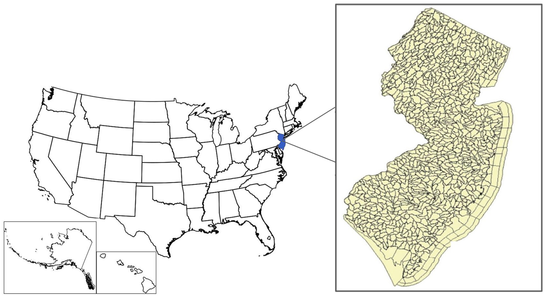
Figure 1. Geographic location of New Jersey with the inset showing the 14-digit hydrologic units (HUC14s) in New Jersey (NJDEP, 2006).

2.2 Study data

Nine input variables – precipitation anomalies, temperature anomalies, precipitation minus evapotranspiration (PME), elevation, topographic slope, natural log of hydraulic conductivity (lnK), long-term mean WTD, GWP, and land cover – were used for predicting either WTD anomalies and/or GWP. Spatial variations of the input data are shown in Figure 2. The input data are grouped into five categories: meteorology- and climatology-related, geology-related, WTD, GWP, and land cover. WTD anomalies calculated from WTD observations and GWP records were used to evaluate the RERF model performance in predicting WTD anomalies and GWP, respectively.

Figure 2

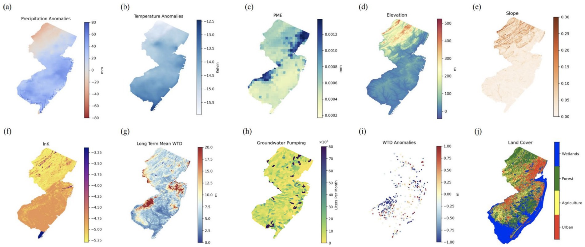
Figure 2. Spatial visualizations of input data for New Jersey, including (A) precipitation anomalies (mm), (B) temperature anomalies (K), (C) precipitation minus evapotranspiration (PME, mm), (D) elevation (m), (E) topographic slope (m), (F) natural log of hydraulic conductivity (lnK), (G) long-term estimated mean WTD (m), (H) GWP (liters per month, L/month), (I) observed WTD anomalies (m), and (J) land cover. The data of precipitation anomalies, temperature anomalies, and GWP are for January 2015 while the observed WTD anomalies are the averages for the years 1990–2020.

2.2.1 Meteorology- and climatology-related data

Three meteorology- and climatology-related inputs, precipitation anomalies, temperature anomalies, and PME (Figures 2A–C), were used in the RERF model and its inverted model. The precipitation anomaly was computed by subtracting the long-term mean precipitation value from the precipitation value. The temperature anomaly was obtained in a similar way. The precipitation and temperature data were from the precipitation and temperature datasets provided by the Center for Western Weather and Water Extremes (CW3E) for the years 1990–2020 (CW3E, 2024), respectively. The PME data was extracted from the potential recharge data utilized in the ParFlow contiguous United States (CONUS) 2.0 platform (Yang et al., 2023), with an initial resolution of 1 km. ParFlow is a parallel, integrated hydrology model that simulates spatially distributed surface and subsurface flow, as well as land surface processes including evapotranspiration and snow (Maxwell et al., 2015).

2.2.2 Geology-related data

As for geology-related data, three inputs were used: elevation, topographic slope, and lnK (Figures 2D–F). The 90 m resolution elevation data were obtained from the seamless USGS 3D Elevation Program digital elevation model dataset (USGS, 2019). The topographic slope was calculated based on the elevation data. The lnK data, in which K had an initial resolution of 1 km, was derived from a continental-scale subsurface K dataset documented in Tijerina-Kreuzer et al. (2023) and Swilley et al. (2023). We averaged K over ten vertical soil and geology layers of varying thicknesses (200, 100, 50, 25, 10, 5, 1, 0.6, 0.3, and 0.1 m from bottom to top) with a depth to bedrock of 392 m, and calculated the nature log of averaged K to obtain lnK.

2.2.3 Water table depth data

WTD observations used in this study were from the United States Geological Survey (USGS) (USGS, 2024), measured in feet. We converted the units to m. They were not available for all of New Jersey, and only certain areas. There were only about 1,250 to 2,100 WTD observations for each year, spread across 288 HUC14s, some areas with more observations than others. The long-term mean WTD was calculated based on WTD measurements since 1914. By subtracting the long-term mean WTD from the WTD observations, WTD anomalies (Figure 2I) were calculated and used as the output variable of the RERF model. As displayed in Figure 2I, positive WTD anomalies indicate increasing WTD while negative WTD anomalies indicate decreasing WTD based on the long-period averages. During prediction, the long-term mean WTD estimates (Figure 2G) in a resolution of 90 m were input to the model to estimate WTD anomalies in grid cells without observations. This was clipped from long-term mean WTD estimates across the CONUS generated using an RF model and all available WTD observations, expanded from the study of Ma et al. (2024).

2.2.4 Groundwater pumping records

GWP used in the study (Figure 2H) was monthly aggregated groundwater withdrawal data from the New Jersey Geological & Water Survey (NJDEP, 2022), measured in million gallons per month. We converted the units to liters per month (L/month). The data was on a HUC14 level and monthly basis from 1990 to 2020. More specifically, there were about 126,000 to 20,000 records of GWP spread across 903 HUC14s or the entire New Jersey state, some HUC14s with more observations than others.

2.2.5 Land cover data

Land cover data (Figure 2J) was used as additional input to the inverted RERF model to predict GWP in New Jersey to improve model performance. Land cover can provide valuable information related to GWP because certain land cover types are correlated to human activities that use groundwater (e.g., agricultural land for irrigation and urban land for industrial uses). The data was for the year of 2015, obtained from the New Jersey Department of Environmental Protection Bureau of GIS (NJDEP Bureau of GIS, 2023b). The original data included a large range of land cover types, such as “residential,” “industrial,” “deciduous forest,” “coniferous forest,” etc., and to reduce the complexity and improve the generalization of unseen data, the land cover categories were limited to four general land cover types: “urban,” “wetlands,” “forests,” and “agriculture.” Additionally, to further normalize the land cover data and have it in a viable form to input into the model, the data was converted into numerical values where “urban” = 1, “wetlands” = 2, “forests” = 3, and “agricultural” = 4. In a total of 56,198,158 grid cells covering New Jersey, 33,065,431 were urban, 116,524,495 were wetland, 8,168,695 were forest, and 3,311,537 were agricultural. Therefore, a large majority, 59%, of the state was considered urban, reflecting the dense population and extensive urban development in the state. To construct the inverted RERF model, a total of 47,280 grid cells with available WTD observations were used, including 20,496 urban grid cells, 16,873 forest grid cells, 6,330 wetland grid cells, and 3,581 agriculture grid cells.

3 Methods

3.1 Regression-enhanced random forest model

The RERF model is an extension of the traditional RF model proposed by Breiman (2001), which encompasses a combination of both RF and Lasso regression (Zhang et al., 2019). The RF model is a type of ML method using ensemble learning. It consists of many decision trees, and each decision tree serves as an independent estimator. The collection of different tree outputs enables the RF model to capture the nonlinear and complex input–output relationship well within the range of the training set (Breiman, 2001; Müller and Guido, 2017). However, as aforementioned, like other tree-based ensemble learning methods, the RF model has poor generalizability to unknown inputs (referred to as the extrapolation issue). Lasso regression is employed to address the issue, which is a type of penalized parametric regression. It is used to capture the global trend within the data in a linear manner (Zhang et al., 2019). In the RERF model, Lasso regression is run first, and then an RF of the residuals is constructed from Lasso, as illustrated in Figure 3.

Figure 3

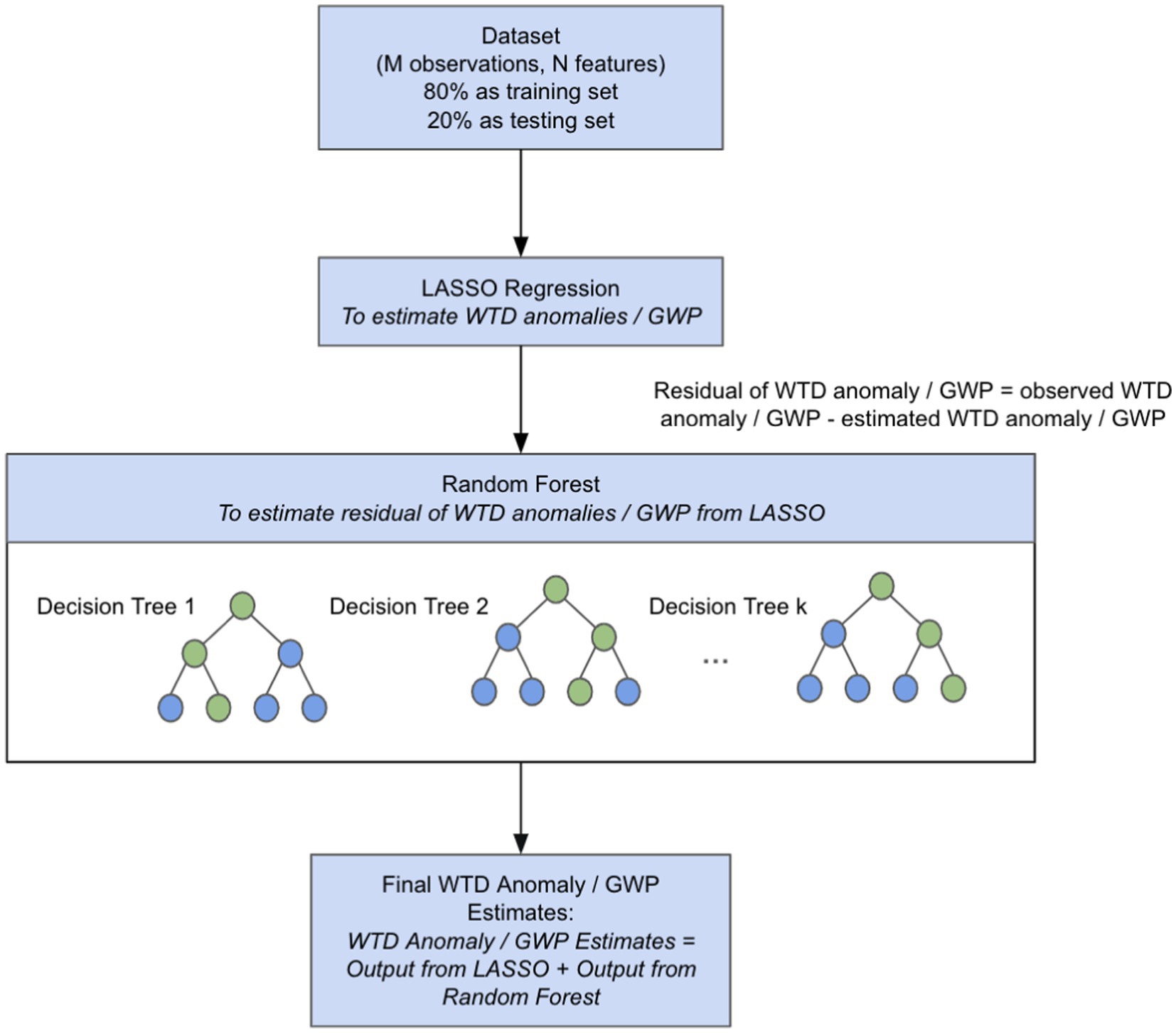
Figure 3. Flow diagram of a regression-enhanced random forest (RERF) model for predicting water table depth (WTD) anomalies or groundwater pumping (GWP).

For predicting WTD anomalies, Lasso regression was trained on observed WTD anomalies. The residual was then calculated by comparing the output from the Lasso regression model and observed WTD anomalies. Then the RF model was trained on the residual. Finally, the outputs of the two models were combined as the final WTD anomaly estimate. For hyperparameters of the RF model, the number of estimators was set to 300 and the maximum tree depth was set to 900, the same as Ma et al. (2024). Eight variables were used as inputs for the model to predict WTD anomalies, which are precipitation anomalies, temperature anomalies, PME, elevation, topographic slope, lnK, long-term mean WTD, and GWP. These predictor variables were selected as factors that can affect groundwater levels. During the model construction, the long-term mean WTD inputs were derived from observed data. A total of 48,719 grid cells with WTD observations were used to train and test the model, with 80% of them randomly selected for training and the other 20% for testing. Later for generating WTD anomalies for the entire state, estimated long-term mean WTD were used. The trained RERF model provides spatiotemporally continuous estimates for WTD anomalies and considers human impacts by including GWP as input.

Then, the RERF model was inverted to use WTD anomalies as input to predict GWP. The input variables except GWP remained consistent with the original RERF model, and land cover data was used as additional input for the model together with WTD anomalies. A cross metric (described in Section 3.2) was also added as input to improve the performance of the inverted RERF model. A total of 48,719 grid cells were used to train and test the inverted model, with 80% of them again randomly selected for training and the other 20% for testing. Observed WTD anomalies were used to construct the model, and during the prediction process, WTD anomalies estimated by the RERF model were fed into the inverted model to produce GWP maps for the entire New Jersey.

3.2 Cross metric

A cross metric was introduced to establish explicit connections between different input variables and to reduce the prediction error in the inverted RERF model. After analyzing the results from the inverted model without the cross metric as input and conducting a trial and error of combining different input variables in the cross metric, the cross metric that produced the highest accuracy involved PME, land cover, WTD anomaly, and the temperature anomaly. More specifically, the cross metric was generated by converting PME, land cover, and the WTD anomaly into binary conditions and then adding them up and multiplying by the temperature anomaly, as expressed in Equation 1.

$\begin{array}{l}\mathrm{Cross\; metric}=\left({\mathrm{P}\mathrm{M}\mathrm{E}}_{\mathrm{b}}+{\mathrm{land\; cover}}_{\mathrm{b}}+\mathrm{W}\mathrm{T}\mathrm{D}{\mathrm{anomaly}}_{\mathrm{b}}\right)\\ \times \mathrm{temperature\; anomaly}\end{array}\text{ (1)}$

where the subscript b represents the binary condition.

For PME, if 0.0005 < PME < 0.0008, PME_b is equal to 1, and otherwise, 0. For land cover, land cover_b is equal to 1 if urban or agriculture, and equal to 0 if wetlands or forest. For WTD anomalies, if −0.1 < WTD anomaly <0.1, WTD anomaly_b is equal to 1, and otherwise, 0. These ranges were based on the analysis presented in the Supplementary material.

3.3 Importance of input variables

The importance of input variables in the RERF model and the inverted model were determined via permutation importance (Breiman, 2001) to show how sensitive the outputs are to different input variables. This method involves randomly shuffling values of each input variable and measuring the decrease in the model performance, which is expressed by the Nash-Sutcliffe Efficiency (NSE) values. Compared to the commonly used SHapley Additive exPlanations (SHAP) values, the permutation importance method provides a very similar rank of input variables based on their relative contributions to the outputs over the entire study domain, but in much less computational time.

3.4 Evaluation metrics

The performances of the RERF model and the inverted model were assessed by comparing the predicted and observed WTD anomaly and GWP predictions, respectively.

For both WTD anomaly and GWP predictions, evaluation metrics, specifically the training and testing NSE, root-squared mean error (RMSE), and Pearson correlation coefficient (r) scores, were calculated using Equations 2–4 to further measure the models’ performances. These metrics provide insights into the model’s predictive performance, with the NSE indicating the model’s ability to capture the variance in the observed data, the RMSE quantifying the average deviation between predicted and observed values, and the r indicating the linear correlation between predicted and observed values.

$\begin{array}{ll}NSE=1-\frac{{{\displaystyle \sum }}_{i=1}^n\left(y_{i-}{\widehat{y}}_i\right)2}{{{\displaystyle \sum }}_{i=1}^n\left(y_{i-}{\overline{y}}_i\right)2}& (2)\end{array}$

$\begin{array}{ll}\mathit{RMSE}=\sqrt{\frac{1}{n}{\displaystyle \sum }_{i=1}^n{\left(y_i-{\widehat{y}}_i\right)}^2}& (3)\end{array}$

$\begin{array}{ll}r=\frac{{{\displaystyle \sum }}_{i=1}^n\left(y_i-\overline{y}\right)\left({\widehat{y}}_i-\overline{\widehat{y}}\right)}{\sqrt{{{\displaystyle \sum }}_{i=1}^n\left(y_i-\overline{y}\right)2{{\displaystyle \sum }}_{i=1}^n\left({\widehat{y}}_i-\overline{\widehat{y}}\right)2}}& (4)\end{array}$

where y_i represents the observed values, ${\widehat{y}}_i$ represents the predicted values, $\overline{y}$ is the mean of the observed values, ${\widehat{\overline{y}}}_i$is the mean of the predicted values, and $n$ is the number of data points.

3.5 Software

The RERF model and its inverted model was developed using scikit-learn, an open-source python library for ML applications (Pedregosa et al., 2011). QGIS is a free and open-source cross-platform desktop geographic information system application that supports the viewing, editing, printing, and analysis of geospatial data (QGIS, 2023). In this study, we applied QGIS 3.34 to identify land cover in each 90 m grid cell.

4 Results and discussion

4.1 Testing model performance in predicting water table depth anomalies and groundwater pumping

Here we built a RERF model using available WTD anomaly observations and input data including GWP, and then inverted the model to predict GWP with WTD anomaly, land cover, and the cross metric introduced in Section 3.2 as additional input. Table 1 lists the testing scores of the RERF model and its inverted model in predicting WTD anomalies and GWP. Both the trained RERF model and the inverted model had acceptable performance dealing with unseen inputs in the testing set, with high r values (> 0.5). The RERF model achieved better scores in predicting WTD anomaly with a test NSE of 0.49, RMSE of 1.61 m, and r of 0.72, while the model for predicting GWP obtained a test NSE of 0.4, RMSE of 15.44 × 10⁶ L/month, and r of 0.65. The relatively poor performance of the inverted model may be attributed to the more heterogeneous pattern of GWP compared to WTD anomalies and additional biases introduced by the inclusion of estimated WTD anomalies.

Table 1

Table 1. Testing Nash-Sutcliffe Efficiency (NSE), root-squared mean error (RMSE), and Pearson correlation coefficient (r) values of the RERF model for predicting water table depth (WTD) anomalies and the inverted model for predicting groundwater pumping (GWP).

Figure 4 compares the estimated and observed values of WTD anomalies and GWP for the test set from 1990 to 2020, which shows variations in the testing performance for individual data points. The data points in Figure 4A are more concentrated on the 1:1 line compared to Figure 4B, which demonstrates again that the model for predicting WTD anomalies outperformed the inverted model for GWP. In Figure 4B, a vertical line of data points is close to the y axis, indicating areas with no or small amount of pumping that were predicted to have higher levels of pumping. We studied the data points on the vertical line and found that they came from 20 HUC14s located in southern New Jersey. Within these HUC14s, there were a mix of high predictions for low observations and low predictions for high observations, which requires further investigation. These false positive predictions greatly contribute to the large RMSE for predicting GWP shown in Table 1.

Figure 4

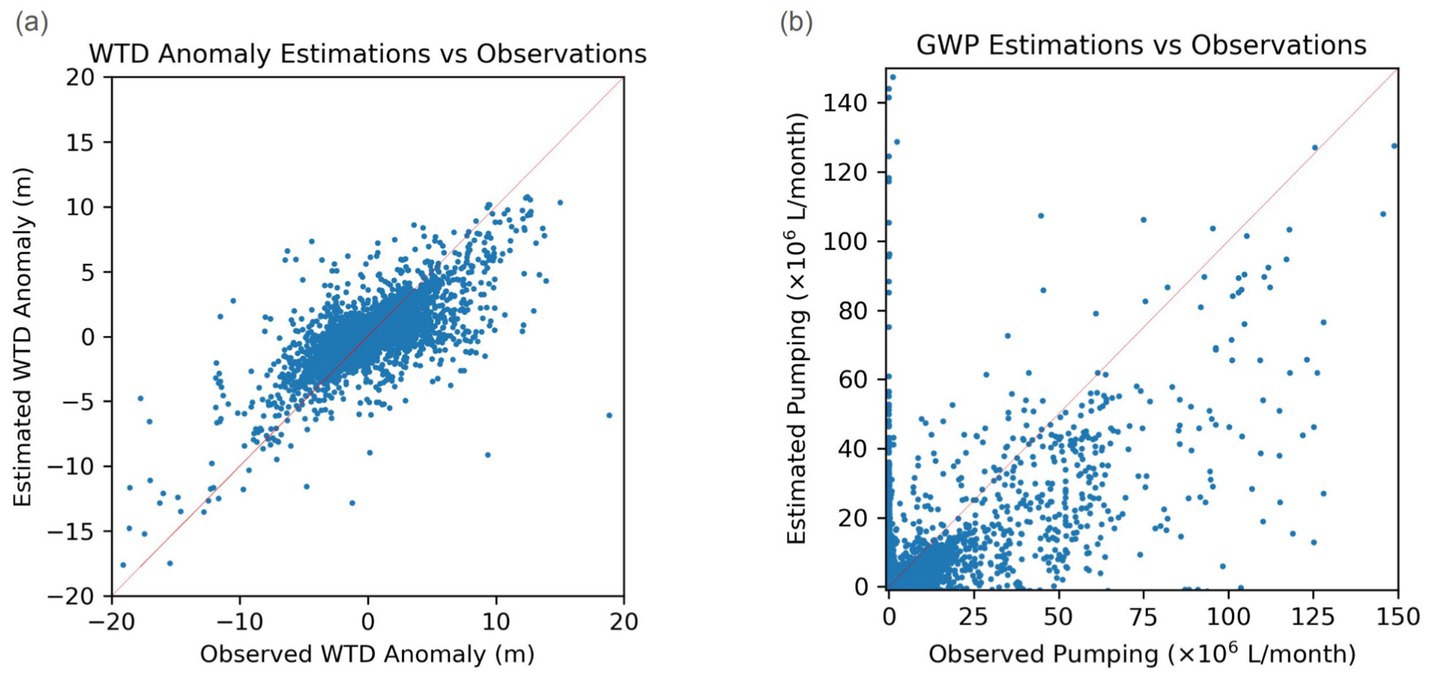
Figure 4. Scatter plots comparing the estimated and observed values of (A) water table depth (WTD) anomalies and (B) groundwater pumping (GWP) during testing. The solid red lines represent lines of 1:1.

4.2 Sensitivity analysis of the models to input variables

We derived the permutation importance of each input variable in both the RERF model and its inverted model (illustrated in Figure 5) to reveal how sensitive the model results were to the input variable.

Figure 5

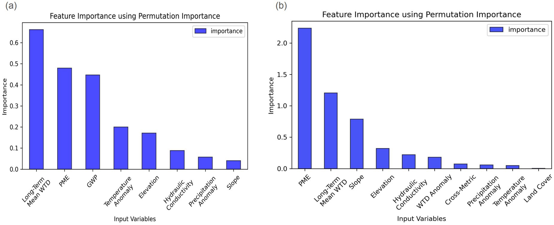
Figure 5. Permutation importance of input variables in the RERF models for predicting (A) water table depth (WTD) anomalies and (B) groundwater pumping (GWP).

Based on Figure 5A, the most important input for predicting WTD anomalies was the long-term mean WTD, which shows how groundwater behaves over a long time. In areas with small long-term mean WTD values (known as shallow groundwater), groundwater systems are typically active in the hydrologic cycle, resulting in frequent changes in WTD anomalies. In contrast, in areas with large long-term mean WTD values (known as deep groundwater), groundwater systems may be disconnected with other components in the hydrologic cycle, leading to rare changes in WTD anomalies if no GWP exists. While the inclusion of the estimated long-term mean WTD during testing introduces additional biases into the estimates, it allows the mapping of WTD anomalies over the entire New Jersey, even for areas without WTD observations. The second most important feature was GWP, which is reasonable as pumping has a direct impact on WTD by extracting groundwater from aquifers and lowering the water table. Hence, more GWP should lead to larger positive WTD anomalies. The third most important feature was PME. PME represents the surplus or deficit of water available in that area after accounting for precipitation and evapotranspiration, the combined process of water evaporation from surfaces and transpiration from plants. The importance of PME for predicting WTD anomalies is consistent with the finding in Condon et al. (2020) that evapotranspiration has a direct effect on groundwater depletion under warming. When PME is a larger value, it suggests either an increased likelihood of groundwater recharge or minimal evapotranspiration, both of which potentially raise the water table. Conversely, smaller or negative values imply a deficit, which could contribute to reduced groundwater recharge, possibly leading to lowered water tables.

As with predicting WTD anomalies (Figure 5A), PME played a critical role in estimating GWP (Figure 5B), more important than the other inputs. PME provides information about groundwater recharge, directly affecting groundwater storage. The significance of PME for predicting GWP suggests that the variations in groundwater recharge strongly affect GWP behavior. The long-term mean WTD was recognized as the second most important input variable. Areas with deeper or shallower mean WTDs may exhibit different groundwater availability and pumping requirements, which can influence GWP patterns. The third most important input variable was slope. Geological data can reflect groundwater flow patterns, infiltration rates, and recharge processes. In the case of slope, areas with higher slope or land steepness may experience faster surface runoff, reduced infiltration, and limited groundwater recharge compared to flatter terrains. Surprisingly, the least important feature was land cover due to its categorical rather than numerical nature. Despite its low permutation importance, land cover still captured important information on GWP activities as it still improved the model performance by a considerable amount. By including land cover, the NSE increased from 0.19 to 0.36; the RMSE decreased from 18.28 × 10⁶ to 15.44 × 10⁶ L/month; and the r increased from 0.52 to 0.62 (Supplementary Table S3). The RF model in the RERF model did not understand the difference between grid cells with a land cover of, e.g., 1 (“urban”), and the ones with a land cover of, e.g., 2 (“wetlands”). In future work, a tree-based model that can better understand categorical inputs, such as LightGBM (Ke et al., 2017), can replace the RF model in the current model.

4.3 Estimated water table depth anomaly and groundwater pumping maps for New Jersey

Using the trained RERF model, we generated estimated 90 m WTD anomaly maps across New Jersey for January and July 2015 (Figures 6, 7, respectively), which are typical winter and summer months. Note that the input long-term mean WTD was replaced by the estimates for the entire state to produce the maps.

Figure 6

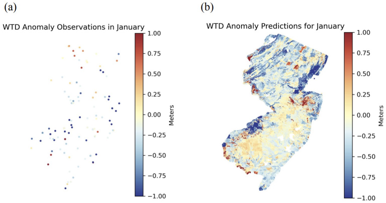
Figure 6. Maps of (A) water table depth (WTD) anomaly observations and (B) WTD anomaly predictions over New Jersey for January 2015.

Figure 7

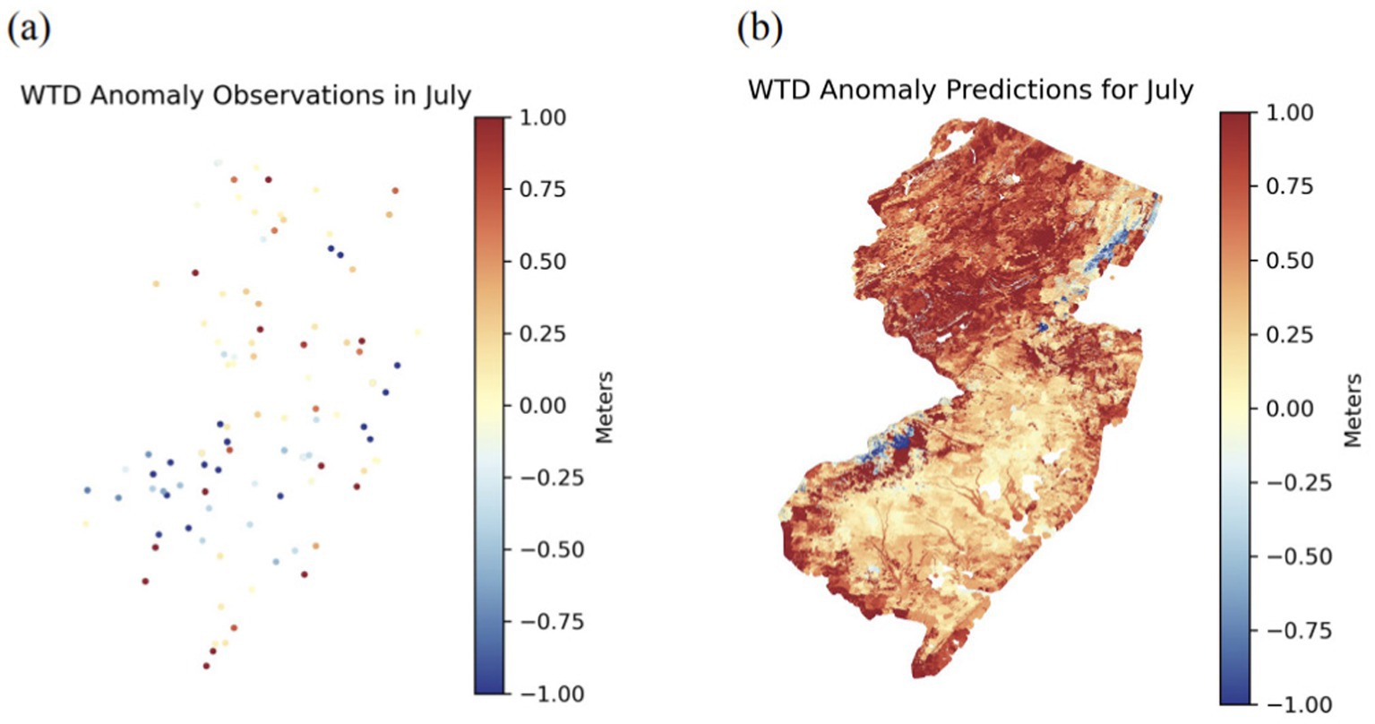
Figure 7. Maps of (A) water table depth (WTD) anomaly observations and (B) WTD anomaly predictions over New Jersey for July 2015.

For January (Figure 6A), the maximum WTD anomaly observation was 7.83 m while the minimum anomaly observation was −11.18 m. The mean anomaly observation was −0.90 m. For January (Figure 6B), the maximum WTD anomaly prediction was found to be 12.22 m while the minimum anomaly prediction was determined to be −8.94 m. The mean anomaly prediction was predicted to be −0.21 m. The small mean value also suggests that the average WTD estimations are similar to the long-term estimated mean WTD and are not particularly low or high in January 2015 since the anomalies represent the difference between them. The standard deviation was also computed to be 0.62 m, so the range of predictions is also relatively small. For July (Figure 7A), the maximum WTD anomaly observed was 7.95 m and the minimum anomaly observed was −11.34 m. The mean anomaly observed was −0.32 m. For July (Figure 7B), the maximum WTD anomaly predicted was found to be 14.46 m while the minimum anomaly predicted was determined to be −5.62 m, which are both higher than for January, indicating lower GWL. The mean anomaly was estimated to be 0.54 m, which was also positive and higher than the mean anomaly for January. However, the standard deviation of 0.61 m was similar to that of January.

While sparse WTD observations exist in New Jersey (Figures 6A, 7A), both maps show reasonable predictions (Figures 6B, 7B) compared to available observations through visual inspection of the colors. For both the observations in Figure 6A and the predictions in Figure 6B for January 2015, the WTD anomalies were negative, meaning that WTD predictions are below the estimated long-term mean WTDs. In other words, there was more groundwater storage than long-term averages. This could potentially be due to typically less GWP and evapotranspiration during the winter than during the rest of the year, thus groundwater levels tend to be higher. For both observations and predictions, very negative WTD anomalies were prominent in the outskirts of New York City or Philadelphia with high urban development. In addition, we also noticed positive WTD anomaly predictions in areas such as the central-eastern region and the southern-western border of New Jersey. Differently, for both the observations in Figure 7A and the predictions in Figure 7B for July 2015 (Figure 7B), the values were predicted to be mainly positive, indicating deeper WTD than the long-term average. This is more likely to happen during the summer than in other seasons, which may contribute to the deeper WTD. Higher positive WTD anomalies are more prominent in the northern parts of New Jersey and along the state’s left border near Philadelphia. Some of these are the same areas that were predicted to have very negative WTD anomalies in January. The discrepancy in WTD anomalies can be due to the increase in temperature during summer, which often leads to lower groundwater recharge, larger GWP, and ultimately higher WTD anomalies. Overall, the WTD anomaly maps reveal changes in groundwater storage in various regions for both cold and warm months and help understand the reasons behind them.

Similarly, we produced estimated GWP maps across New Jersey for the same months using the trained inverted RERF model, as shown in Figures 8, 9. To predict GWP for the entire state, the estimated WTD anomaly outputs from the RERF model were used as input as WTD observations are only available for a few grid cells. We summed up GWP for each HUC14 to compare with original GWP records.

Figure 8

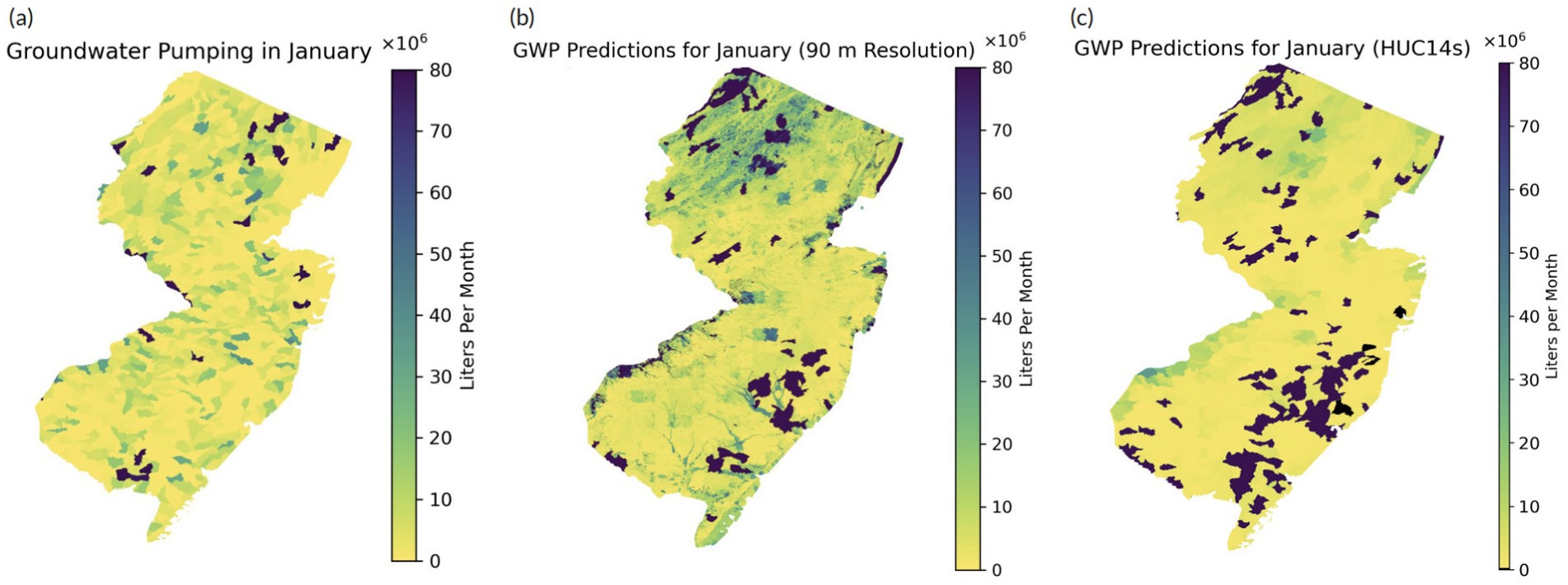
Figure 8. Maps of (A) groundwater pumping (GWP) records at the HUC14 level, (B) GWP predictions in a 90 m resolution, and (C) summed GWP predictions at the HUC14 level over New Jersey for January 2015 measured in liters per month (L/month).

Figure 9

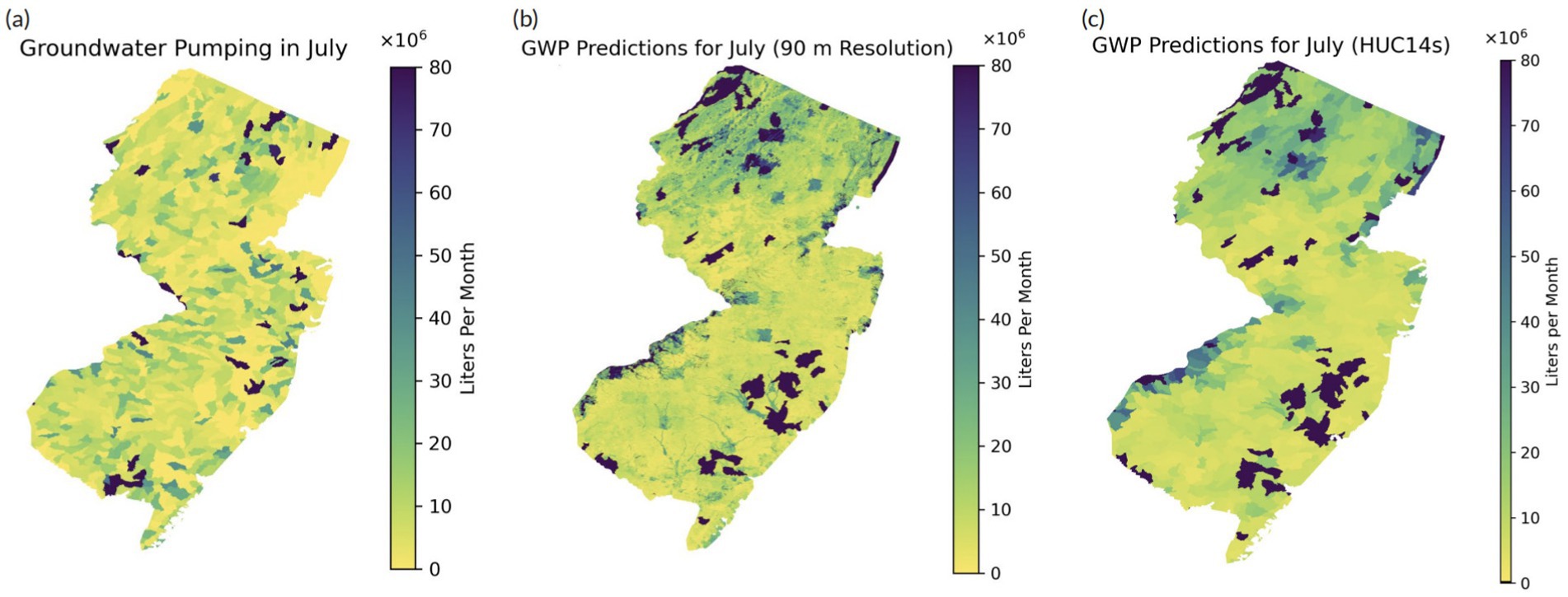
Figure 9. Maps of (A) groundwater pumping (GWP) records at the HUC14 level, (B) GWP predictions in a 90 m resolution, and (C) summed GWP predictions at the HUC14 level over New Jersey for July 2015 measured in liters per month (L/month).

While in Figure 8A, the GWP observations are randomly distributed, in Figures 8B,C, the model predictions suggest higher GWP rates in northern New Jersey and near the suburbs of New York City and Philadelphia. Extremely high GWP rates were found in a few areas spread across the state indicated by their dark colors. Similar results are found in Figure 9 for July. These discrepancies between observed and predicted pumping patterns may stem from limitations or uncertainties in the model, such as inaccurate input data and potentially missing input data. It is important to note that the estimated GWP data have much higher resolution than the GWP records, and the different scales may also be attributed to the discrepancies in Figures 8, 9.

For January, the maximum predicted pumping value was 331.48 × 10⁶ L/month. The minimum predicted value was 0.53 × 10⁶ L/month, meaning that the model never predicted a GWP value of 0 despite being trained on sites where there was 0 GWP. The mean predicted value was 49.13 × 10⁶ L/month. These values do not completely align with the observed pumping values as the maximum value was much higher at 1804.55 × 10⁶ L/month and the minimum value was 0 L/month, respectively. The mean observed value was found to be 14.39 × 10⁶ L/month. For July, the maximum predicted pumping value was 507.91 × 10⁶ L/month. The minimum predicted value was 2.61 × 10⁶ L/month, and again the model never predicted a GWP value of 0. The mean predicted value was 51.26 × 10⁶ L/month. Once again, these values are not that close with the observed pumping values, especially the maximum observed value, which was 1994.91 × 10⁶ L/month. The minimum observed value was 0 L/month, and the mean observed value was 18.71 × 10⁶ L/month. As expected, the mean predicted GWP for July was slightly higher than the mean prediction for January. This is further supported by the darker colors in Figure 9 than in Figure 8, indicating higher pumping rates. Additionally, in both cases, the maximum predicted GWP value was decently high, raising questions about the model’s potential for outliers or inaccuracies in the predictions.

Overall, the better model performance for predicting WTD anomalies than for predicting GWP may be attributed to a more direct input–output relationship in the former model. GWP often results in groundwater depletion and increasing WTD, as illustrated in Kuang et al. (2024) and Figure 5A. Conversely, GWP is an anthropogenic activity closely linked to socio-economic development (e.g., urbanization), and does not necessarily change as a result of WTD and WTD anomalies. Thus, for predicting GWP, the long-term mean WTD was not the most important input variable, and the WTD anomaly had little contribution to the predictions (as shown in Figure 5B). There were a considerable amount of false positives in the results for predicting GWP (as shown in Figure 4B), which can only be slightly eliminated by adding the cross metric (described in Section 3.2) as input. The large number of false positives may indicate missing information in the inverted model, which requires further investigation.

In addition, a critical contributor to the model’s acceptable WTD anomaly predictions was the integration of GWP data as input. GWP was the third most important input variable (Figure 5A), emphasizing the value of incorporating pumping information to groundwater resource modeling when pumping records are available. Indeed, the RERF model with GWP as input outperformed the one without GWP as input (Supplementary Table S2). As a coastal state, the WTD in New Jersey is generally shallow (as shown in Figure 2G), and groundwater is actively involved in the hydrologic cycle. Therefore, we also observed non-zero WTD anomalies in areas with zero GWP in Figures 6, 7, which were impacted by the meteorology- and climatology-related inputs. Constructing RERF models in mountainous regions with deep groundwater may lead to different findings.

Although we only showed estimated WTD anomaly and GWP maps for New Jersey in January and July 2015 (Section 4.3), the trained RERF model and inverted RERF model can be employed to produce WTD anomaly and GWP maps for any month during 1990–2020 at a high spatial resolution (i.e., 90 m). Based on the spatiotemporally continuous WTD anomaly and GWP estimates during 1990–2020, we can gain some insights into the impact of climate change on both WTD anomalies and GWP in a coastal region like New Jersey. This can be an application of the developed models.

5 Conclusion

In this study, we built RERF models to estimate WTD anomalies and GWP for a coastal state in the United States, New Jersey, based on available WTD observations, long-term mean WTD estimates, meteorology- and climatology-related data, geology-related data, GWP data, and land cover data. The RERF model for predicting WTD anomalies had a test NSE of 0.49, RMSE of 1.61 m, and r of 0.72, while the inverted RERF model for predicting GWP with the cross metric as additional input had a test NSE of 0.40, RMSE of 15.44 × 10⁶ L/month, and r of 0.65. The top three important inputs for predicting WTD anomalies were long-term mean WTD, PME, and GWP, while the top three important inputs for predicting GWP were the PME, long-term mean WTD, and topographic slope. Using the trained models, we generated WTD anomaly and GWP maps for New Jersey for January and July 2015, which are the winter and summer months of an average year without many extreme events. As a coastal state with shallow groundwater, most areas in New Jersey had small WTD anomalies within the range between −1 m and 1 m. GWP showed a more heterogeneous pattern in New Jersey than WTD anomalies. Overall, the RERF models offer insights into groundwater availability and pumping capacity in coastal states like New Jersey, of which groundwater systems are vulnerable to GWP. Based on the findings, the study demonstrates that even though the RERF models have room for improvement, they can be effective in producing acceptable estimates for WTD anomalies and GWP, serving as a viable alternative for predicting in areas with limited or unavailable WTD observations.

As aforementioned, the RERF models have some limitations and can be further improved. As data-driven models, their predictions are highly affected by the quality and quantity of the given data. Sparse WTD monitoring wells with long records (Figure 2I) constrained the model behavior. As many of the grid cells with WTD observations were around the Philadelphia suburbs, the models were trained on mostly urban areas with similar geological and climate conditions. Along with the spatial restriction, the temporal limitation of WTD data may also introduce biases, as it could be concentrated in certain years or months. There were very few grid cells with monthly continuous WTD observations over a long time period. Hence, increasing WTD observations and training on a larger diverse range of grid cells and a longer time period may improve the model performance. Also, utilizing predicted WTD anomalies instead of observed WTD anomalies to generate GWP maps for the entire New Jersey can introduce additional errors to the inverted model, as the WTD anomaly predictions are usually different from the observations. We noticed that the RF model in the RERF model somehow failed to understand categorical data such as land cover, resulting in its low importance rank. Moreover, the importance of the input variable to the output variable cannot demonstrate the causal relationship between the input and output variables, which can also be due to external drivers (Tesch et al., 2023). Future work can focus on studying and resolving some of the uncertainties, issues, and challenges encountered within the scope of this study. For instance, one path of exploration is to continuously test different inputs and cross metrics for the RERF model and its inverted model to improve the model performance. One can also replace the RF model in the RERF model with a ML method that understands various types of data, such as LightGBM. Assuming that New Jersey has a similar hydrogeological setting and pumping conditions to other regions, the RERF models trained for New Jersey, without additional training, may be extrapolated to these regions to predict WTD anomalies and GWP. This is known as domain adaptation in ML terminology (Pan et al., 2011). Extending the RERF models to predict WTD anomalies and GWP in other regions can help assess the generalizability of the models. One can also link the WTD and GWP predictions from the developed model to sea level rise to better understand seawater intrusion in New Jersey during the study period. Hence, by leveraging advanced computational algorithms and existing datasets, ML models can enable accurate and timely groundwater level and quality predictions, which then can enhance groundwater monitoring and management practices and inform future decision-making processes.

Code availability statement

The Jupyter notebooks predicting WTD anomalies and GWP using the RERF model are available at: https://github.com/jamiekk2002/RERF_Model.

Data availability statement

The original contributions presented in the study are included in the article/Supplementary material, further inquiries can be directed to the corresponding authors.

Author contributions

JK: Formal analysis, Methodology, Validation, Visualization, Writing – original draft, Writing – review & editing. YM: Conceptualization, Data curation, Methodology, Supervision, Writing – original draft, Writing – review & editing. RM: Conceptualization, Supervision, Writing – review & editing, Funding acquisition.

Funding

The author(s) declare that financial support was received for the research, authorship, and/or publication of this article. This research has been supported by the U.S. National Science Foundation Convergence Accelerator Program (grant no. CA-2040542). The authors also wish to acknowledge the support from the Princeton University High Meadows Environmental Institute Environmental Internship Program (JK).

Conflict of interest

The authors declare that the research was conducted in the absence of any commercial or financial relationships that could be construed as a potential conflict of interest.

Generative AI statement

The author(s) declare that no Generative AI was used in the creation of this manuscript.

Publisher’s note

All claims expressed in this article are solely those of the authors and do not necessarily represent those of their affiliated organizations, or those of the publisher, the editors and the reviewers. Any product that may be evaluated in this article, or claim that may be made by its manufacturer, is not guaranteed or endorsed by the publisher.

Supplementary material

The Supplementary material for this article can be found online at: https://www.frontiersin.org/articles/10.3389/frwa.2024.1509945/full#supplementary-material

References

Ahmadi, A., Olyaei, M., Heydari, Z., Emami, M., Zeynolabedin, A., Ghomlaghi, A., et al. (2022). Groundwater level modeling with machine learning: a systematic review and Meta-analysis. Water 14:949. doi: 10.3390/w14060949

Crossref Full Text | Google Scholar

Belitz, K., and Stackelberg, P. E. (2021). Evaluation of six methods for correcting bias in estimates from ensemble tree machine learning regression models. Environ. Model Softw. 139:105006. doi: 10.1016/j.envsoft.2021.105006

Crossref Full Text | Google Scholar

Boo, K. B. W., El-Shafie, A., Othman, F., Khan, M. M. H., Birima, A. H., and Ahmed, A. N. (2024). Groundwater level forecasting with machine learning models: a review. Water Res. 252:121249. doi: 10.1016/j.watres.2024.121249

PubMed Abstract | Crossref Full Text | Google Scholar

Breiman, L. (2001). Random forests. Mach Learn 45, 5–32. doi: 10.1023/A:1010933404324

Crossref Full Text | Google Scholar

Che Nordin, N. F., Mohd, N. S., Koting, S., Ismail, Z., Sherif, M., and El-Shafie, A. (2021). Groundwater quality forecasting modelling using artificial intelligence: a review. Groundw. Sustain. Dev. 14:100643. doi: 10.1016/j.gsd.2021.100643

Crossref Full Text | Google Scholar

Condon, L. E., Atchley, A. L., and Maxwell, R. M. (2020). Evapotranspiration depletes groundwater under warming over the contiguous United States. Nat. Commun. 11:873. doi: 10.1038/s41467-020-14688-0

PubMed Abstract | Crossref Full Text | Google Scholar

CW3E (2024). Center for Western Weather and Water Extremes. Available at:https://cw3e.ucsd.edu/. Accessed February 14, 2024.

Google Scholar

De Filippi, F. M., Ginesi, M., and Sappa, G. (2024). A fully connected neural network (FCNN) model to simulate karst spring flowrates in the Umbria region (Central Italy). Water 16:2580. doi: 10.3390/w16182580

Crossref Full Text | Google Scholar

de Graaf, I. E. M., Gleeson, T., (Rens) van Beek, L. P. H., Sutanudjaja, E. H., and Bierkens, M. F. P. (2019). Environmental flow limits to global groundwater pumping. Nature 574, 90–94. doi: 10.1038/s41586-019-1594-4

PubMed Abstract | Crossref Full Text | Google Scholar

Gholami, V., Chau, K. W., Fadaee, F., Torkaman, J., and Ghaffari, A. (2015). Modeling of groundwater level fluctuations using dendrochronology in alluvial aquifers. J. Hydrol. 529, 1060–1069. doi: 10.1016/j.jhydrol.2015.09.028

Crossref Full Text | Google Scholar

Green, T. R., Taniguchi, M., Kooi, H., Gurdak, J. J., Allen, D. M., Hiscock, K. M., et al. (2011). Beneath the surface of global change: impacts of climate change on groundwater. J. Hydrol. 405, 532–560. doi: 10.1016/j.jhydrol.2011.05.002

Crossref Full Text | Google Scholar

Han, D., and Currell, M. J. (2022). Review of drivers and threats to coastal groundwater quality in China. Sci. Total Environ. 806:150913. doi: 10.1016/j.scitotenv.2021.150913

PubMed Abstract | Crossref Full Text | Google Scholar

Jasechko, S., Perrone, D., Seybold, H., Fan, Y., and Kirchner, J. W. (2020). Groundwater level observations in 250,000 coastal US wells reveal scope of potential seawater intrusion. Nat. Commun. 11:3229. doi: 10.1038/s41467-020-17038-2

PubMed Abstract | Crossref Full Text | Google Scholar

Jasechko, S., Seybold, H., Perrone, D., Fan, Y., Shamsudduha, M., Taylor, R. G., et al. (2024). Rapid groundwater decline and some cases of recovery in aquifers globally. Nature 625, 715–721. doi: 10.1038/s41586-023-06879-8

PubMed Abstract | Crossref Full Text | Google Scholar

Ke, G., Meng, Q., Finely, T., Wang, T., Chen, W., Ma, W., et al. (2017). LightGBM: a highly efficient gradient boosting decision tree. Adv. Neural Infor. Proces. Syst. 30, 3149–3157.

Google Scholar

Kollet, S. J., and Maxwell, R. M. (2008). Capturing the influence of groundwater dynamics on land surface processes using an integrated, distributed watershed model. Water Resour. Res. 44. doi: 10.1029/2007WR006004

Crossref Full Text | Google Scholar

Konikow, L. F., and Kendy, E. (2005). Groundwater depletion: a global problem. Hydrogeol. J. 13, 317–320. doi: 10.1007/s10040-004-0411-8

Crossref Full Text | Google Scholar

Kuang, X., Liu, J., Scanlon, B. R., Jiao, J. J., Jasechko, S., Lancia, M., et al. (2024). The changing nature of groundwater in the global water cycle. Science 383:eadf0630. doi: 10.1126/science.adf0630

PubMed Abstract | Crossref Full Text | Google Scholar

Ma, Y., Leonarduzzi, E., Defnet, A., Melchior, P., Condon, L. E., and Maxwell, R. M. (2024). Water table depth estimates over the contiguous United States using a random Forest model. Groundwater 62, 34–43. doi: 10.1111/gwat.13362

Crossref Full Text | Google Scholar

Ma, Y., Montzka, C., Bayat, B., and Kollet, S. (2021). Using Long short-term memory networks to connect water table depth anomalies to precipitation anomalies over Europe. Hydrol. Earth Syst. Sci. 25, 3555–3575. doi: 10.5194/hess-25-3555-2021

Crossref Full Text | Google Scholar

Ma, Y., Montzka, C., Naz, B. S., and Kollet, S. (2022). Advancing AI-based pan-European groundwater monitoring. Environ. Res. Lett. 17:114037. doi: 10.1088/1748-9326/ac9c1e

Crossref Full Text | Google Scholar

Maxwell, R. M., Condon, L. E., and Kollet, S. J. (2015). A high-resolution simulation of groundwater and surface water over most of the continental US with the integrated hydrologic model ParFlow v3. Geosci. Model Dev. 8, 923–937. doi: 10.5194/gmd-8-923-2015

Crossref Full Text | Google Scholar

Müller, A. C., and Guido, S. (2017). Ensembles of Decision Trees. Introduction to machine learning with Python: A guide for data scientists, (Sebastopol: O’Reilly Media, Inc.), 85–94.

Google Scholar

NJDEP (2006). 14 Digit Hydrologic Unit Code Delineations for New Jersey (Version 20110225). Available at: https://www.nj.gov/dep/gis/digidownload/metadata/statewide/dephuc14.htm (Accessed September 30, 2024).

Google Scholar

NJDEP (2022). DGS 10–3 New Jersey water transfer model withdrawal, use, and return data summaries. New Jersey geological and water survey. Available at: https://dep.nj.gov/njgws/digital-data/dsg-10-3/ (Accessed June 6, 2023).

Google Scholar

NJDEP Bureau of GIS (2023a). 14 Digit Hydrologic Unit Code Delineations for New Jersey. Available at:https://gisdata-njdep.opendata.arcgis.com/datasets/njdep::14-digit-hydrologic-unit-code-delineations-for-new-jersey/about. Accessed June 6, 2024.

Google Scholar

NJDEP Bureau of GIS (2023b). Land Use/Land Cover of New Jersey 2015 (Download). Available at:https://gisdata-njdep.opendata.arcgis.com/documents/6f76b90deda34cc98aec255e2defdb45/about. Accessed June 6, 2024.

Google Scholar

Pan, S. J., Tsang, I. W., Kwok, J. T., and Yang, Q. (2011). Domain adaptation via transfer component analysis. IEEE Trans. Neural Netw. 22, 199–210. doi: 10.1109/TNN.2010.2091281

PubMed Abstract | Crossref Full Text | Google Scholar

Peters, C. N., Kimsal, C., Frederiks, R. S., Paldor, A., McQuiggan, R., and Michael, H. A. (2022). Groundwater pumping causes salinization of coastal streams due to baseflow depletion: analytical framework and application to Savannah River, GA. J. Hydrol. 604:127238. doi: 10.1016/j.jhydrol.2021.127238

Crossref Full Text | Google Scholar

Pedregosa, F., Varoquaux, G., Gramfort, A., Michel, V., Thirion, B., Grisel, O., et al. (2011). Scikit-learn: Machine Learning in Python. J Mach Learn Res. 12, 2825–2830.

Google Scholar

Pölz, A., Blaschke, A. P., Komma, J., Farnleitner, A. H., and Derx, J. (2024). Transformer versus LSTM: a comparison of deep learning models for karst spring discharge forecasting. Water Resour. Res. 60. doi: 10.1029/2022WR032602

Crossref Full Text | Google Scholar

QGIS (2023). QGIS geographic information system : Open Source Geospatial Foundation Project.

Google Scholar

Rodell, M., Famiglietti, J. S., Wiese, D. N., Reager, J. T., Beaudoing, H. K., Landerer, F. W., et al. (2018). Emerging trends in global freshwater availability. Nature 557, 651–659. doi: 10.1038/s41586-018-0123-1

PubMed Abstract | Crossref Full Text | Google Scholar

Rodell, M., and Reager, J. T. (2023). Water cycle science enabled by the GRACE and GRACE-FO satellite missions. Nature Water 1, 47–59. doi: 10.1038/s44221-022-00005-0

Crossref Full Text | Google Scholar

Rosecrans, C. Z., Belitz, K., Ransom, K. M., Stackelberg, P. E., and McMahon, P. B. (2022). Predicting regional fluoride concentrations at public and domestic supply depths in basin-fill aquifers of the western United States using a random forest model. Sci. Total Environ. 806:150960. doi: 10.1016/j.scitotenv.2021.150960

PubMed Abstract | Crossref Full Text | Google Scholar

Sahoo, M., Kasot, A., Dhar, A., and Kar, A. (2018). On predictability of groundwater level in shallow Wells using satellite observations. Water Resour. Manag. 32, 1225–1244. doi: 10.1007/s11269-017-1865-5

Crossref Full Text | Google Scholar

Sarkar, S., Das, K., and Mukherjee, A. (2024). Groundwater salinity across India: predicting occurrences and controls by field-observations and machine learning modeling. Environ. Sci. Technol. 58, 3953–3965. doi: 10.1021/acs.est.3c06525

PubMed Abstract | Crossref Full Text | Google Scholar

Scanlon, B. R., Fakhreddine, S., Rateb, A., de Graaf, I., Famiglietti, J., Gleeson, T., et al. (2023). Global water resources and the role of groundwater in a resilient water future. Nat Rev Earth Environ. 4, 87–101. doi: 10.1038/s43017-022-00378-6

Crossref Full Text | Google Scholar

Sun, A. Y. (2013). Predicting groundwater level changes using GRACE data. Water Resour. Res. 49, 5900–5912. doi: 10.1002/wrcr.20421

Crossref Full Text | Google Scholar

Swilley, J. S., Tijerina-Kreuzer, D., Tran, H. V., Zhang, J., Yang, C., Condon, L. E., et al. (2023). Continental scale Hydrostratigraphy: comparing geologically informed data products to analytical solutions. Groundwater 62, 75–92. doi: 10.1111/gwat.13354

PubMed Abstract | Crossref Full Text | Google Scholar

Tao, H., Hameed, M. M., Marhoon, H. A., Zounemat-Kermani, M., Heddam, S., Kim, S., et al. (2022). Groundwater level prediction using machine learning models: a comprehensive review. Neurocomputing 489, 271–308. doi: 10.1016/j.neucom.2022.03.014

Crossref Full Text | Google Scholar

Taylor, C. S., and Alley, W. M. (2001). Ground-water-level monitoring and the importance of Long-term water-level data (circular 1217). U.S. Geological Survey. Available at:https://pubs.usgs.gov/circ/circ1217/pdf/circular1217.pdf

Google Scholar

Tesch, T., Kollet, S., and Garcke, J. (2023). Causal deep learning models for studying the earth system. Geosci. Model Dev. 16, 2149–2166. doi: 10.5194/gmd-16-2149-2023

Crossref Full Text | Google Scholar

Tijerina-Kreuzer, D., Swilley, J. S., Tran, H. V., Zhang, J., West, B., Yang, C., et al. (2023). Continental scale Hydrostratigraphy: basin-scale testing of alternative data-driven approaches. Groundwater 62, 93–110. doi: 10.1111/gwat.13357

PubMed Abstract | Crossref Full Text | Google Scholar

United States Census Bureau (2021). 2020 Census Apportionment Results. Available at:https://www.census.gov/data/tables/2020/dec/2020-apportionment-data.html (Accessed June 6, 2024).

Google Scholar

USGS (2019). The National map—new Data Delivery Homepage, advanced viewer, Lidar visualization. Reston, VA: USGS.

Google Scholar

USGS (2024). USGS Groundwater Data for New Jersey. Available at:https://waterdata.usgs.gov/nj/nwis/gw (Accessed June 6, 2024).

Google Scholar

van Engelen, J., Essink, G. H. P. O., and Bierkens, M. F. P. (2022). Sustainability of fresh groundwater resources in fifteen major deltas around the world. Environ. Res. Lett. 17:125001. doi: 10.1088/1748-9326/aca16c

Crossref Full Text | Google Scholar

Vu, M. T., Jardani, A., Massei, N., and Fournier, M. (2021). Reconstruction of missing groundwater level data by using Long short-term memory (LSTM) deep neural network. J. Hydrol. 597:125776. doi: 10.1016/j.jhydrol.2020.125776

Crossref Full Text | Google Scholar

Wunsch, A., Liesch, T., and Broda, S. (2022). Deep learning shows declining groundwater levels in Germany until 2100 due to climate change. Nat. Commun. 13:1221. doi: 10.1038/s41467-022-28770-2

PubMed Abstract | Crossref Full Text | Google Scholar

Yang, C., Tijerina-Kreuzer, D. T., Tran, H. V., Condon, L. E., and Maxwell, R. M. (2023). A high-resolution, 3D groundwater-surface water simulation of the contiguous US: advances in the integrated ParFlow CONUS 2.0 modeling platform. J. Hydrol. 626:130294. doi: 10.1016/j.jhydrol.2023.130294

Crossref Full Text | Google Scholar

Zhang, H., Nettleton, D., and Zhu, Z. (2019). Section on Statistical Learning and Data Science. Alexandria, VA: Am. Stat. Assoc. 636–647. doi: 10.48550/arXiv.1904.10416

Crossref Full Text | Google Scholar