Reinforcement learning for watershed and aquifer management: a nationwide view in the country of Mexico with emphasis in Baja California Sur

Reinforcement Learning (RL) is a method that teaches agents to make informed decisions in diverse environments through trial and error, aiming to maximize a reward function and discover the optimal Q-learning function for decision-making. In this study, we apply RL to a rule-based water management simulation, utilizing a deep learning approach for the Q-learning value function. The trained RL model can learn from the environment and make real-time decisions. Our approach offers an unbiased method for analyzing complex watershed scenarios, providing a reward function as an analytical metric while optimizing decision-making time. Overall, this work underscores RL’s potential in addressing complex problems, demanding exploration, sequential decision-making, and continuous learning. External variables such as policy shifts, which are not readily integrated into the model, can substantially influence outcomes. Upon establishing a model with the requisite minimal states and actions, the subsequent learning process is relatively straightforward, depending on the selection of appropriate RL model algorithms. Its application depends on the specific problem. The primary challenge in this modeling approach lies in model definition, specifically in devising agents and actions that apply to complex scenarios. Our specific example was designed to address recent decision-making challenges related to constructing dams due to water scarcity. We present two examples: one from a nationwide perspective in Mexico and the other focused on Baja California Sur, the state with the highest water stress. Our results demonstrate our capability to prioritize watersheds effectively for the most significant benefits, particularly dam construction.

1 Introduction

Water management plays a crucial role in ensuring the sustainability of cities and addressing various challenges related to water use, scarcity minimization, and sustainability performance. Water distribution networks encompass a complex web of components and activities, from aqueduct planning to leak repair and modeling, all aimed at efficiently transporting water to households, businesses, and public facilities. The management of water resources is a global concern, with implications for policy and stakeholders worldwide (Savenije and Van Der Zaag, 2005; Gorelick and Zheng, 2015; Ingold and Tosun, 2020; Ramos et al., 2020).

Particularly critical is the management of aquifers in arid regions, given their pivotal role in maintaining water availability and quality. Effective policies are essential for sustainable aquifer use, mitigating depletion risks (Chichilnisky and Heal, 1993; Mohtadi, 1996) and preserving ecosystems dependent on groundwater resources (Huang and Uri, 1990). Aquifer management often involves navigating legal obligations, environmental regulations, socioeconomic factors, and ethical considerations, making it a complex task. Traditional static or rule-based strategies may fall short in adapting to changing conditions or capturing the intricate dynamics of aquifer systems.

In response to these challenges, new technologies such as RL have emerged as a promising avenue for optimizing public policy (Binas et al., 2019; Strnad et al., 2019; Chen et al., 2021; Skirzyński et al., 2021; Emamjomehzadeh et al., 2023; Ghobadi and Kang, 2023; Sivamayil et al., 2023). RL allows computers to learn from experience, enabling intelligent decision-making in complex environments (Lee et al., 2022). In this context, we focus on simulating a water management system that allows an autonomous agent the opportunity to learn through trial-and-error interactions driven by reward signals.

The primary objective of this study is to explore the application of RL techniques in groundwater management, specifically in determining the necessity of investigating an aquifer for dam construction in arid regions while addressing internal issues and striving to maintain a delicate balance between water network maintenance, the construction of dams, and the development of aqueducts, all while optimizing these efforts to ensure efficient water management. Incorporating the assessment of technical, economic, and ecological factors into dam projects aligns well with an RL approach. RL can adaptively balance these diverse considerations, optimizing dam planning, especially in arid regions where benefits often surpass ecological concerns, ensuring effective and sustainable strategies. We propose a reward structure and state-action representations that capture the dynamics and tradeoffs within aquifer systems using rule-based environments that directly validate agent decisions.

Reinforcement learning is well-suited for sequential decision-making to maximize cumulative rewards (Santoro et al., 2016; Strnad et al., 2019; Sivamayil et al., 2023). It leverages the Q-learning algorithm to enable the agent to learn an optimal strategy by estimating the action value function (Q-function) through environmental interactions. For temporal problems, RL employs temporal difference learning, allowing the agent to learn from experience over time. The Q-function iteratively updates based on the difference between predicted and observed rewards, continuously refining the agent’s decision-making capabilities.

Notably, RL has found applications in various water-related domains, including water distribution, heating, water metering, and reservoir operation (Castelletti et al., 2010; Ruelens et al., 2018; Hu et al., 2020, 2022; Amasyali et al., 2021; Chen and Ray, 2022; Khampuengson and Wang, 2022). However, integrating rule-based environments within RL for water management simulations is new. It offers several advantages, enhancing adaptability and learning capacity, such as: (a) Incorporating Expert Knowledge: Rule-based environments encapsulate domain-specific expertise, preventing catastrophic errors and accelerating learning. (b) Safety and Compliance: Enforcing regulations and safety measures ensures ethical and environmentally responsible decision-making. (c) Providing a Baseline: Rule-based environments offer a foundational understanding for RL agents before exploring more complex strategies. (d) Rapid Prototyping and Testing: Rule-based systems enable quick prototyping and testing, as they do not rely on deploying complex city sensors, saving time and resources.

The most significant difficulty in this type of modeling is defining the model itself that is, creating agents and actions that are useful and applicable to a problem of this complexity. For example, we might be tempted to use states like lithology, permeability, and hydraulic conductivity, but these states could be encompassed in a single state called “modeling.” On the other hand, a state that cannot be included, such as changes in the city’s external policies, could have a considerable impact. The learning part is relatively straightforward once the model has been defined and the minimum number of states and actions has been determined. It simply requires choosing the appropriate algorithms to solve the RL model.

The definition of states and actions in any policy is inherently driven by its specific goal, and this goal cannot be universally applied to all management scenarios. For instance, when the aim is to construct a dam, the focus naturally shifts toward defining states and actions that optimize the construction process. However, this approach is not directly applicable to other objectives, like reducing water consumption. In this new scenario, strategies should focus on conservation measures, monitoring usage, and encouraging reduced consumption behaviors. Varying goals demand distinct plans. We must make particular strategies for each goal and understand the problem.

We used an example that was custom-made for a specific situation. This example was designed to address the challenges that emerged when the government of Mexico started building aqueducts, but we need to study aquifers to manage water resources effectively. The main idea is to demonstrate how a particular method can benefit stakeholders. So, this specific case illustrates our approach to tackling complex issues, showing its potential applicability in various situations.

First, this paper presents the mathematical formalism in the methodology section. Then, we have three main sections: “Environment,” “Deep Q-Learning” (DQN), and “ε-Greedy.” These sections focus on mathematical algorithms related to rule-based RL presented in the methodology section. We offer two examples: one showcasing a nationwide application in Mexico and the other demonstrating a more detailed focus on Baja California Sur.

2 Methodology

Reinforcement learning can be explained mathematically as Markov Decision Processes (MDPs, Bellman, 1957). An MDP is an extension of Markov chains that involves decision-making and actions taken by an agent to maximize cumulative rewards over time. Like Markov chains, MDPs are based on a fixed set of states, where each represents the current environment situation. With MDPs, the agent can take actions to influence state transitions and achieve specific goals. The agent’s actions determine the probability of transitioning to different states. MDPs contain rewards associated with state transitions and actions. The agent’s goal is to learn a strategy that maximizes the cumulative rewards achieved over time.

In RL, we formalize the process as a MDP with the following components:

1. A set of states, S, and a distribution of initial states, $p\left(s\right)$ .

2. A series of actions, $A\in a$ .

3. Dynamics of transitions, $T\left(s_{t+1}\mathrm{|,}{s}_t\mathrm{|,}{a}_t\right)$ , which is the probability distribution of the next state at time $t+1$ taking into account the state and the action at time $t$ .

4. An immediate reward function, $R\left(s_t\mathrm{,}{a}_t\mathrm{,}{s}_{t+1}\right)$specifies the reward that is obtained when moving from state $s_t$ to $s_{t+1}$after execution of the action $a_t$ .

5. A discount factor, $\gamma \in \left[0\mathrm{,}1\right]$ with lower values favoring immediate rewards.

The value of a state $s$ under the policy $\pi ,$ abbreviated as $V^{\pi }\left(s\right)$is the expected return on investment in the state $s$ and under the policy $\pi .$ The discounted model with an infinite time horizon can be expressed as follows:

$\begin{array}{ll}{V}^{\pi }\left(s\right)=E_{\pi }\left\{{\displaystyle \sum }_{k=0}^{\infty }{\gamma }^k{r}_{t+k}|s_t\right\}=E_{\pi }\left\{s\right\}& (1)\end{array}$

Thereby $\gamma$ is a discount factor and $E_{\pi }\left\{\cdot \right\}$ is an optimal value, $k$ stands for time steps, $r_{t+k}$ denotes the rewards to be gained in the transition to the state $s_t$and the expected value is related to the policy $\pi .$

Similarly, a state action value function $Q:S\times A\to ℝ$ can be defined as the expected yield starting from the state $s$ with the action $a,$ and then the following policy $\pi$ :

$\begin{array}{ll}{Q}_{\pi }\left(s\mathrm{,}a\right)=E_{\pi }\left\{{\displaystyle \sum }_{k=0}^{\infty }{\gamma }^k{r}_{t+k}|s_t\mathrm{,}{a}_t\right\}=E_{\pi }\left\{s\mathrm{,}a\right\}& (2)\end{array}$

where $a_t$ denotes the action to be taken in the next state $s$ after the policy $\pi$ .

A fundamental property of value functions is their recursive nature. For each policy $\pi$ and each state $s$ , the expression in Equation (2) can be defined recursively using the Bellman equation (Bellman, 1957):

$V^{\pi }\left(s\right)=E_{\pi }\left\{r_t+\gamma r_{t+1}+{\gamma }^2{r}_{t+2}+\dots |s_t=t\right\}$

$=E_{\pi }\left\{r_t+\gamma V^{\pi }\left(s_{t+1}\right)|s_t=s\right\}$

$\begin{array}{ll}={\displaystyle \sum }_{s\prime }T\left(s\mathrm{,}\pi \left(s\right)\mathrm{,}{s}^{\prime }\right)R\left(s\mathrm{,}a\mathrm{,}{s}^{\prime }\right)+\gamma V^{\pi }\left(s^{\prime }\right)& (3)\end{array}$

The Bellman equation states that the expected value of a state is defined by the immediate reward and the values of possible following states, weighted by their transition probabilities and by a discount factor. $V^{\pi }$ is the only solution to these equations. It is worth noting that several strategies can have the same value function, but for a given strategy π, $V^{\pi }$ is unique. It follows that the optimal strategy is:

$\begin{array}{ll}{V}^{\ast }\left(s\right)=\underset{a}{\max }{\displaystyle \sum }_{s\prime }T\left(s\mathrm{,}\pi \left(s\right)\mathrm{,}{s}^{\prime }\right)R\left(s\mathrm{,}a\mathrm{,}{s}^{\prime }\right)+\gamma V^{\pi }\left(s^{\prime }\right)& (4)\end{array}$

This expression is known as the Bellman optimality equation, which states that the value of a state under an optimal policy must equal the expected return for the best action in that state. For organizational purposes, the terms are $T\left(s\mathrm{,}\pi \left(s\right)\mathrm{,}{s}^{\prime }\right)R\left(s\mathrm{,}a\mathrm{,}{s}^{\prime }\right)$are elaborated in a section labeled Environment, while the $\gamma V^{\pi }\left(s^{\prime }\right)$ and the final calculation $V^{\ast }\left(s\right)$ is performed in another section called Agent. However, $R\left(s\mathrm{,}a\mathrm{,}{s}^{\prime }\right)$ which is the reward function where the environment receives the action, is not always a deterministic function, but in the real world behaves like a stochastic function with a probability of

$\begin{array}{ll}E\left\{R\left(s\mathrm{,}a\mathrm{,}{s}^{\prime }\right)\right\}={\displaystyle \sum }_{r}P\left(r\mathrm{|}s\mathrm{,}a\mathrm{,}{s}^{\prime }\right)\times r& (5)\end{array}$

$P\left(r\mathrm{|}s\mathrm{,}a\mathrm{,}{s}^{\prime }\right)$ is the probability of receiving a reward r when the agent takes action from the state s and transitions to state s′. r is a specific reward value that can be received.

Several challenges in RL deserve attention. (1) Discovering the optimal strategy requires trial-and-error interactions with the environment, and the agent’s learning signal is the reward it receives. (2) Its actions influence the agent’s observations and can have significant temporal correlations. (3) Agents must deal with extensive temporal dependencies, where the consequences of an action may only become apparent after several environmental transitions. This is referred to as the temporal credit allocation problem.

We examine these challenges in building a dam to supply water to a city. While the end goal of aquifer investigation and dam design may be clear, the exact sequence of actions required is uncertain. Long-term processes involve challenges such as population growth and severe droughts that could affect decision-making. To find the optimal course of action, we must balance exploration with learning from the consequences of our experiments over time.

3 Environment

The environment manages rules for actions. At its core, the primary function of the environment is to receive an action from the agent, which is implemented as a neural network along with a learning algorithm. The main task of the environment is to check the validity of the action provided by the agent and then generate the corresponding new state. This process is illustrated in Figure 1. Five state variables were deliberately chosen because they can distinguish different levels that contribute to the evaluation of the state of the aquifer and the environment, including the population center. We encapsulated the environment in a class that uses the OpenAI Gym framework (Brockman et al., 2016). This class provides a structured and standardized way to interact with the environment, allowing seamless integration with other components and facilitating an organized and efficient implementation.

Figure 1

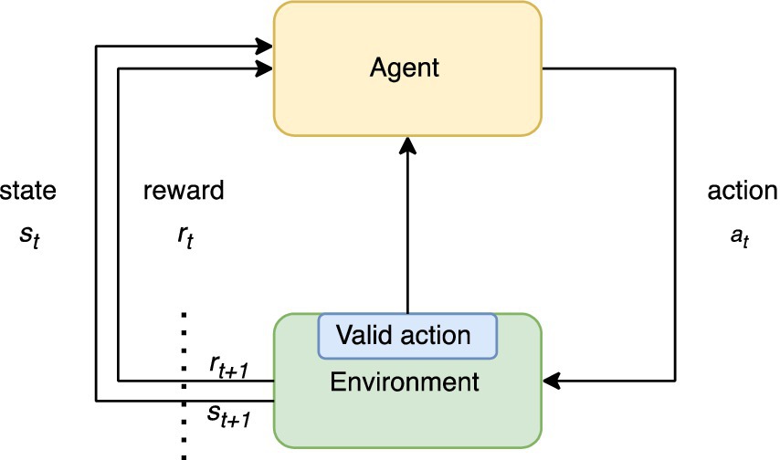
Figure 1. Sequence of the reinforcement learning process. At time t, the environment receives an action, which is validated and results in a change of state “s” with reward function “r.” It is then updated as a new state reward input to the agent (DQN). The environment checks if the action is valid and sends a signal to the agent.

Starting from scratch could lead to excessive work and a higher chance of errors. Instead, using OpenAI Gym saves time by providing ready-to-use tools. This platform was chosen for its thorough testing, accessibility, universality, scalability, and ease of debugging. However, no hard-coded routines were used; only the provided framework was utilized. Other platforms, such as Sci-Kit Learn or Tensorflow (Abadi et al., 2016), have the capabilities of Deep Learning, but none of them have coded agent-environment interactions. We wrote all the necessary functions so our results would be the same on any platform. The only difference is the organization of the code.

Essentially, the environment is designed to simulate a natural physical environment. This environment relies on sensors that measure changes such as temperature or pressure for smart home appliances. In the case of ruled-based, the environment is simulated with clear and well-structured relations with states and actions.

Our main goal is to build dams sustainably. Our environment is rule-based and includes four states: “Annual Volume,” “Availability,” “Distance,” “Necessity,” and “Modeling.” These states have the following meanings: (1) Annual volume refers to the amount of water in the aquifer, measured in hectometers. This parameter remains nearly constant across all actions, except for the transition to “construction of dams,” the action that directly affects this state. Although these levels change throughout the year and even over several decades, in terms of public policy, the source used to analyze the aquifer is based on a study called “Mean Annual Availability,” which in turn treats this variable as a constant number that assumes that this availability does not vary. For this reason, this value is considered constant. (2) Availability represents the total amount of water withdrawn from the annual water volume of the aquifer. The resulting value represents the amount of water remaining in the aquifer and available for various purposes such as irrigation, drinking water supply and industrial use. This parameter can take either positive or negative values depending on whether there is a water deficit or surplus. This calculation is essential for managing and maintaining sustainable use of groundwater resources. When water withdrawal exceeds the natural rate, overuse and depletion of the aquifer occur, leading to serious environmental problems and water scarcity in the region. (3) Distance is the measurement in kilometers between the water source and populated areas. The distance may change after constructing an aqueduct, which is a practical value affecting policy. In other words, if there is already an aqueduct, this aquifer can be used similarly if another aquifer is nearby. (4) Necessity represents the water demand of the nearest heavily populated area, measured in liters per second (l/s). (5) Modeling is a level that quantifies the level of understanding of the aquifer and is expressed on a scale of 0–100. It reflects progress in 3D groundwater modeling, the maturity of studies conducted, and advances in geophysical, geologic, and hydrologic research. This measure is an abstract representation and is always presented as a fraction of the total knowledge required to build a dam. Various variables were explored, such as lithology, porosity, and climate, which are natural and physical factors influential in the situation. However, the aim was to go beyond and directly consider the involved society. The goal was to make a decision that not only took into account the purely physical aspects of the environment but also those directly related to the affected community. This implies understanding how the decision would impact people, their specific needs, and concerns. In summary, a more holistic approach focused on people, rather than solely relying on geological or environmental factors, was sought.

Our model differs from classic RL because the environment can sense and decide if an action is valid. This has several important reasons. First, in our mathematical framework (Equation 4), there is no requirement for a separate function between the environment and the agent. Both the environment and the agent play equal roles in the MDP. Additionally, the environment plays a crucial role in validating actions and determining if they should lead to a new state and reward. In our case, the environment is represented as a rule-based physical simulation, such as a city with people, sensors, and needs. The actions correspond to policy decisions, such as those made by city councils. Consequently, the environment can either accept or reject actions. This is not unusual because, in real life, various mechanisms exist for accepting and validating actions after they have been taken. For instance, legal protections may apply to specific political actions, or environmental regulations not initially considered may affect the agent’s decisions.

The actions are divided into four categories: (a) “Repairing leaks,” (b) “Building aqueducts,” (c) “Building dams,” and (d) “Conducting studies.” These actions were carefully chosen to influence states while serving as common approaches to address water scarcity in the driest regions with high water stress.

The environment not only updates the state when receiving actions from the agent but also performs essential quality control and testing of the action state. This is mathematically and physically accepted because the environment constantly interacts with the agent in real life. It also computes a reward function that plays a central role in controlling the learning process. In some cases, the environment contains stochastic elements that introduce random events, simulating the variability of the real world. These stochastic factors mimic situations where the environment might react differently than rule-based expectations. For example, dams might be built without proper studies, or due to tax policy or leakage. Another example is that repairs might be delayed even though they were needed.

However, we want to simulate the optimal solution of Q-learning to ensure an accurate representation of the optimal solution. With this approach, we can focus on finding the best possible actions and the appropriate rewards to achieve the desired Q-learning outcome.

The reward is a simple function that relates the value of the states and evaluates them in terms of cost. The reward function considers the aspects of volume, availability, distance, necessity, and modeling of the environment. It encourages the agent to prefer actions that increase the volume and availability of water while minimizing the distance and necessity. Defined as:

$\begin{array}{l}reward=A\times volume+B\times availability-\left(C\times distance\right)-\\ \left(D\times necessity\right)+E\times modelling\end{array}$

Where, $A=1,B=0.001,C=10,D=1,E=20$ . The differences in scale are adjusted to achieve a balanced and consistent reward multifactor function in hectometer, lt/s, and percent units. This ensures that each factor contributes meaningfully to the total reward despite the inherent differences in their scales. Given the Monte Carlo and Variance-Based sensitivity analysis results, we observe a dynamic interaction between input variables and their impact on the system’s output. The Monte Carlo simulation (Figure 2), showcasing a broad distribution of rewards, suggests a significant influence on our parameters, highlighting the model’s sensitivity. This wide distribution is crucial because the reward function can show significant variations when selecting an action. Concurrently, the Variance-Based analysis provides a deeper understanding of each variable’s contribution to the output variance. The first-order sensitivity indices reveal the most critical parameters, guiding us toward areas requiring precise calibration or robust data collection. These analyses offer a comprehensive view of the system’s behavior, enabling targeted adjustments to enhance model reliability and decision-making efficacy in complex scenarios.

Figure 2

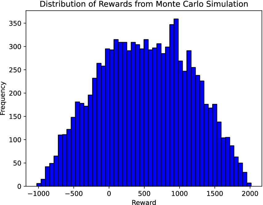
Figure 2. Sensitivity analysis using a Monte Carlo simulation, a broad distribution of rewards suggests a significant influence on our parameters highlighting the model’s sensitivity.

The following sections will incorporate the reward function into the learning process. By assigning rewards for different actions and states, the agent will be able to identify the most favorable choices that lead to higher rewards and, consequently, better performance.

4 Deep Q-learning

Learning an optimal strategy can be done in different ways; Bellman’s dynamic programming is the most common way. Bellman’s dynamic programming is a fundamental approach in RL that breaks down decision-making processes into simpler sub-problems. It relies on the principle of optimality, which asserts that the optimal policy can be derived by making optimal decisions based on the current and future states at each stage. This approach is advantageous for problems with a discrete and finite state space, where the entire decision process can be systematically analyzed and solved. The major strength of Bellman’s method is its comprehensiveness and precision in finding the optimal solution through recursion and backward induction. However, its primary drawback is the “curse of dimensionality”; as the state and action spaces expand, the computational resources and time required to compute the solution increase exponentially, making it impractical for complex, high-dimensional problems.

Another option besides dynamic programming is DQN, which combines RL with deep neural networks, leveraging the approximation capabilities of deep learning to estimate the value function. This approach allows handling environments with high-dimensional state spaces, making it well-suited for tasks like image-based problems where traditional methods falter. DQNs can generalize across states, reducing the need to explicitly compute the value of each state-action pair, which significantly mitigates the curse of dimensionality. However, DQNs introduce challenges, such as the need for large amounts of data to effectively train the neural network, the risk of overfitting, and the complexity of tuning network architectures and hyperparameters. Moreover, the black-box nature of neural networks makes the decision-making process less interpretable than Bellman’s dynamic programming.

In our case, a neural network model is trained using the Tensorflow Keras library (Abadi et al., 2016) to learn an optimal strategy for actions that affect state variables. Figure 3 shows the neural network’s architecture that is trained to obtain an action based on states. DQNs combine Deep Learning and Q-learning elements to handle complex, high-dimensional state spaces, making them particularly effective for tasks where traditional Q-learning approaches may become impractical or inefficient.

Figure 3

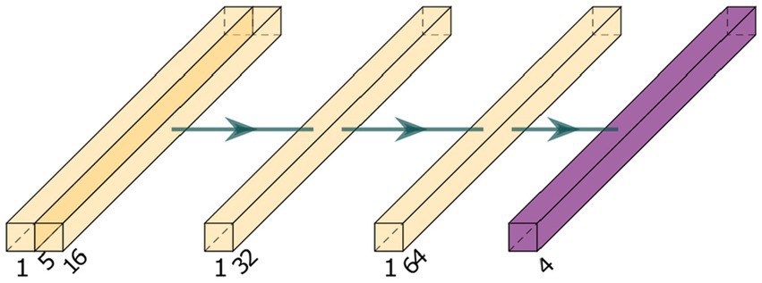
Figure 3. The architecture of the DQN neural network consists of three fully connected layers and a final softmax connection. During the training process, the network is controlled by a reward function while interacting with the environment.

The network consists of four layers with different numbers of neurons and activation functions. The first layer includes 16 neurons and expects input with five features. The ReLU activation function adds nonlinearity to the network and improves its ability to learn complicated relationships. The second layer consists of 32 neurons and uses ReLU activation. The third layer includes 64 neurons with ReLU activation. Finally, the output layer consists of four neurons corresponding to the four actions in the environment, respectively. Using the activation function “Softmax,” this layer converts the output values into a probability distribution for the actions. The neural network is designed to accept a state representation with five features as input and generate action probabilities from which the agent can choose. With ReLU activation when learning complex Q-value relationships and softmax activation, the architecture is best suited for RL tasks using the DQN methodology.

Figure 4 shows the outlines of a generic training loop for RL. It involves iteratively training an agent through multiple episodes in an environment. During each episode, the agent selects actions based on its current state and a learned strategy. The actions can be selected by exploration (random) or exploitation (based on the predictions of the strategy). The agent then observes the next state and immediate reward from the environment. The rewards are normalized to a consistent range. The algorithm updates its internal model or Q-values based on the observed transitions to improve the agent’s strategy. The process is repeated for a specified number of episodes, storing the cumulative rewards achieved in each episode. Ultimately, the training loop aims to optimize the agent’s strategy to maximize cumulative rewards over time.

Figure 4

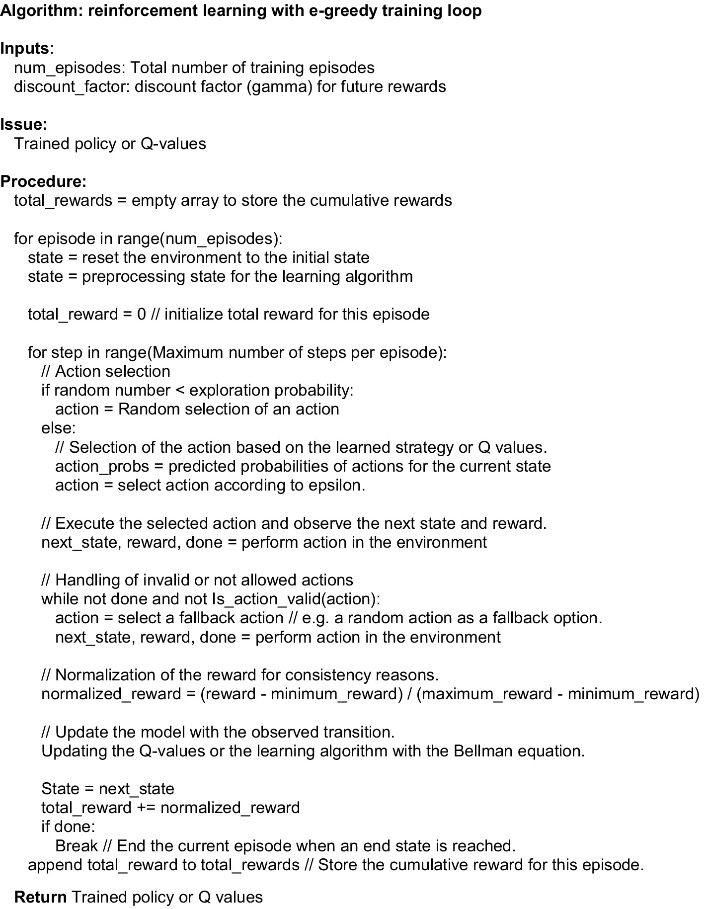
Figure 4. RL training loop with ε-greedy-exploration-transition.

5 ε-Greedy

ε-Greedy is an exploration and exploitation strategy agents use to make decisions in uncertain environments. ε-Greedy was chosen because it can switch to new actions when the agent exploits a particular strategy. For example, repair leaking or modeling states were often exploited without a balance in the agents’ decisions so needed to strike a balance between trying new actions (exploration) and exploiting the best-known actions (exploitation) to maximize long-term rewards. We added the ε-Greedy strategy to balance all the decisions; the ε-Greedy strategy is simple and easy to implement (Figure 5). At each time step “t,” the agent selects an action according to the following rule:

1. With a probability of ε (epsilon), the agent chooses a random action from the set of available actions. This promotes exploration by allowing the agent to try different actions and learn more about the environment.

2. With probability (1 − ε), the agent exploits its current knowledge and chooses the action with the highest estimated reward based on previous experience. Exploitation aims to take advantage of the actions shown to yield higher rewards.

Figure 5

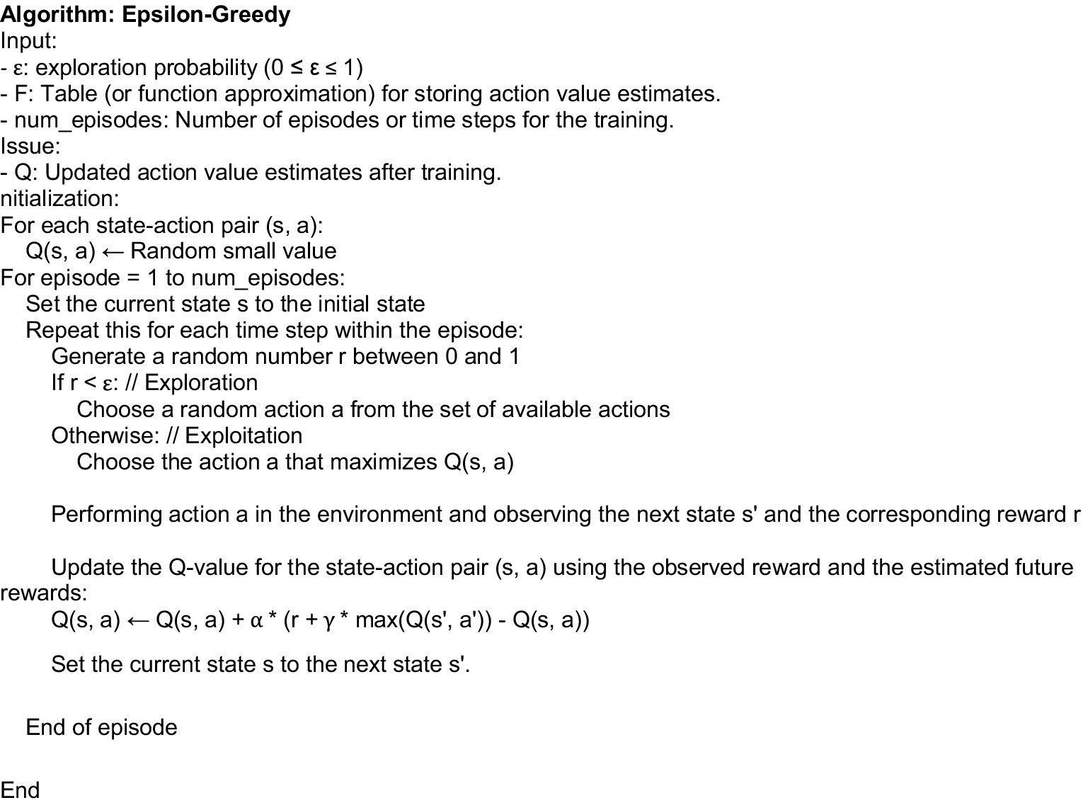
Figure 5. ε-Greedy. The random part represents the exploration section where different options are searched.

By adjusting the value of ε, an agent can control the degree of exploration versus exploitation. A higher ε-value encourages more exploration, while a lower ε-value tends toward more exploitation. The main advantage of ε-Greedy is its simplicity and versatility. It is a nonparametric approach that requires no assumptions about the underlying environment. In addition, ε-Greedy is computationally efficient, making it suitable for a wide range of applications. However, ε-Greedy also has some drawbacks. A significant limitation is that it treats all actions during exploration as equally uncertain, which may not be the case in complex environments. It may be suboptimal in situations where some actions are worth exploring more than others.

To address this constraint, alternatively, different forms of ε-Greedy have been suggested, including implementing a decreasing ε schedule. The idea is to start with a high ε-value to explore more at the beginning of the learning process, gradually decreasing this value over time, focusing more on exploitation as the agent gains more experience. Although ε-Greedy and Metropolis-Hastings are different algorithms used in different contexts (RL and Markov chain Monte Carlo methods, respectively), they have some conceptual similarities when considering their connections to MDPs and Markov chains. Both the ε-Greedy and Metropolis-Hasting methods involve a tradeoff between exploration and exploitation. In ε-Greedy, the agent weighs between exploring new actions (with probability ε) and using the currently known best actions (with probability 1 − ε) during the decision process in an MDP. In Metropolis-Hastings, the algorithm weighs between exploring new states (by proposing transitions to new states with a certain probability) and using states with higher probability (by accepting or rejecting the proposed transitions based on the acceptance probability) during the sampling process in a Markov chain. In ε-Greedy, the agent randomly chooses an action (with probability ε) during exploration rather than always choosing the best-known action. This stochastic introduces exploration and ensures the agent is not stuck in a suboptimal strategy.

In ε-Greedy, the agent’s decision-making is based on the current state of the environment, which satisfies the Markov property of MDPs. The agent does not need to maintain a history of past states to make decisions. In ε-Greedy, as the agent collects more data through interactions with the environment, it is expected to converge to the optimal action—value function (Q-function) or strategy for the MDP.

The model’s performance is evaluated by testing it in the environment and selecting actions based on the highest predicted action probability. Our final code can be obtained in Ortega, (2024).

6 Implementation

In Figure 6, we depict the states and actions that were illustrated in our RL process. The states (1) Annual Volume, (2) Necessity, (3) Availability, (4) Distance, and (5) Modeling interact with the actions: (a) Repair leaking, (b) Construction of aqueducts, (c) Dam construction, and (d) Perform studies. Note that states and actions are intrinsically connected, for example, the action Repair leaking with Necessity and Construction of aqueducts with Distance.

Figure 6

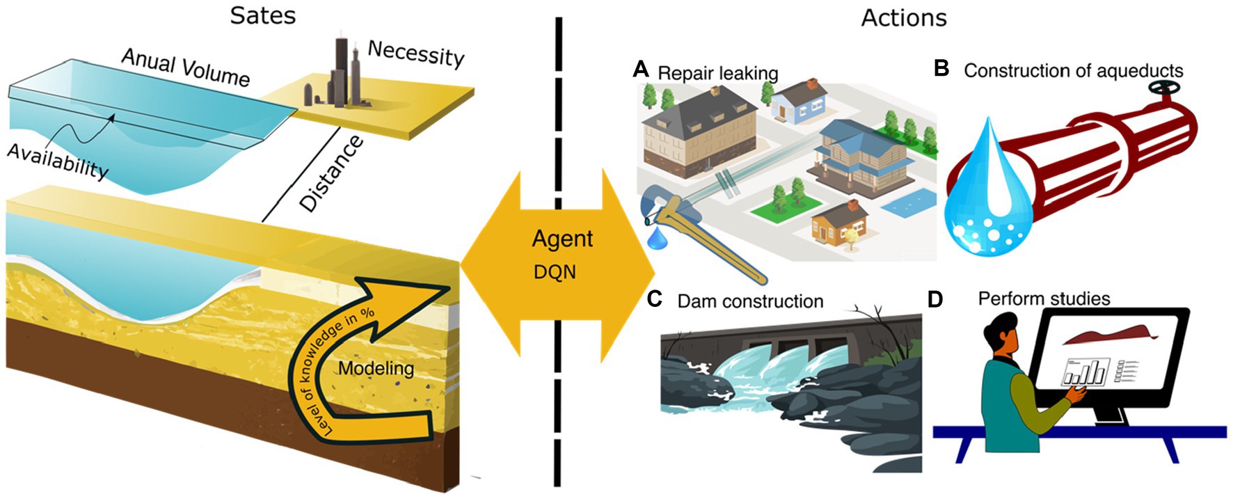
Figure 6. Illustration of states and actions of this specific example. The states and actions are intrinsically connected; for example, action “Perform studies” with “Modeling” and “Construction of aqueducts with Distance.” The agent receives states and decides an action based on a function DQN. Internally, there is a reward function that controls the efficiency of the RL process.

Unlike other machine learning methods that focus on accuracy without guiding the learning process, RL aims to teach the agent how to learn and make good decisions in its environment. During training, the agent explores the environment and refines its understanding of state transitions and action sequences. Thus, in RL, how we learn is more important rather than merely focusing on accuracy. The RL’s iterative nature and adaptive approach allow for continuous updating of strategies based on feedback from the environment, making it different from traditional supervised learning. Further research and experiments can extend this approach to more complex environments.

The Environment class simulates a water management system with five continuous state variables, each with specific ranges. The neural network model is built using Tensorflow Keras (Abadi et al., 2016) and consists of three hidden layers with 16, 32, and 64 neurons, respectively, and a final output layer with four neurons corresponding to the discrete actions. The model is trained to predict the action probabilities based on the current state, learning the optimal environmental strategy. In the training loop, episodes are run to gain experience and update the model based on the observed transitions. Rewards are calculated using the coefficient-based reward function, highlighting the importance of each state variable. The model’s performance is evaluated by testing it in the environment and selecting actions based on the highest predicted action probabilities.

Model complexity is generally strongly related to training stability (Hu et al., 2021). The initial state is chosen for the city of La Paz, Mexico, which is the capital city of Baja California Sur. In RL, a step is a single interaction between the agent and its environment. During each step, the agent selects an action, and the environment responds by transitioning to a new state and providing a reward signal. This action-state-reward cycle is fundamental to RL algorithms, and the agent often updates its policy or value function based on the outcomes of these steps. In Q-learning, the agent updates its Q-values after each step.

Conversely, an episode refers to a sequence of steps that begins with an initial state and concludes when a predefined terminal condition is met. Episodes are a way to structure RL tasks and define when the agent has completed a specific task or goal. The termination of an episode could be due to reaching a goal state (infinite time horizon), exceeding a maximum number of steps (finite time horizon), or encountering a particular event. Also, epochs pertain to the training process of DQN neural networks. During each epoch, the entire training dataset is passed through the neural network forward and backward. Deep learning models are typically trained over multiple epochs to enhance their performance. The number of epochs is a hyperparameter that can be adjusted based on the model’s convergence behavior.

In Figure 7, we provide an instance of the total reward function across various episodes. Decision changes are significant just before the learning trend stabilizes, meaning decision policies compete to establish a learning trend. For this reason, episodes 1–7 show variability in the four actions. Figure 7 displays all learning episodes to demonstrate that the trend has begun to stabilize. The increase in rewards signifies that the RL agent is learning from its interactions with the environment and is finding better strategies or policies over time. As it accumulates experience, it becomes better at selecting actions that lead to higher rewards (exploitation). At the same time, the RL process may have found a good balance between exploration (trying new actions) and exploitation (choosing known good actions) to maximize rewards.

Figure 7

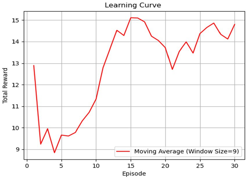
Figure 7. The learning curve illustrates the agent’s performance based on the total reward function in each episode. After episode 10, the agent shows significant progress, indicating an increased level of learning.

Since the DQN starts without knowledge, the reward function slowly performs better until it has the optimal behavior. However, we found that the reward function does not always behave the same way because it depends on the initial random state. We can estimate the Q-value (Figure 8) at each episode depending on the different actions. Decision changes are significant just before the learning trend stabilizes, meaning decision policies compete to establish a learning trend. For this reason, episodes 1–7 show variability in the four actions. Note that Figure 7 displays all learning episodes to demonstrate that the trend begins to stabilize, but Figure 8 enhances those changes.

Figure 8

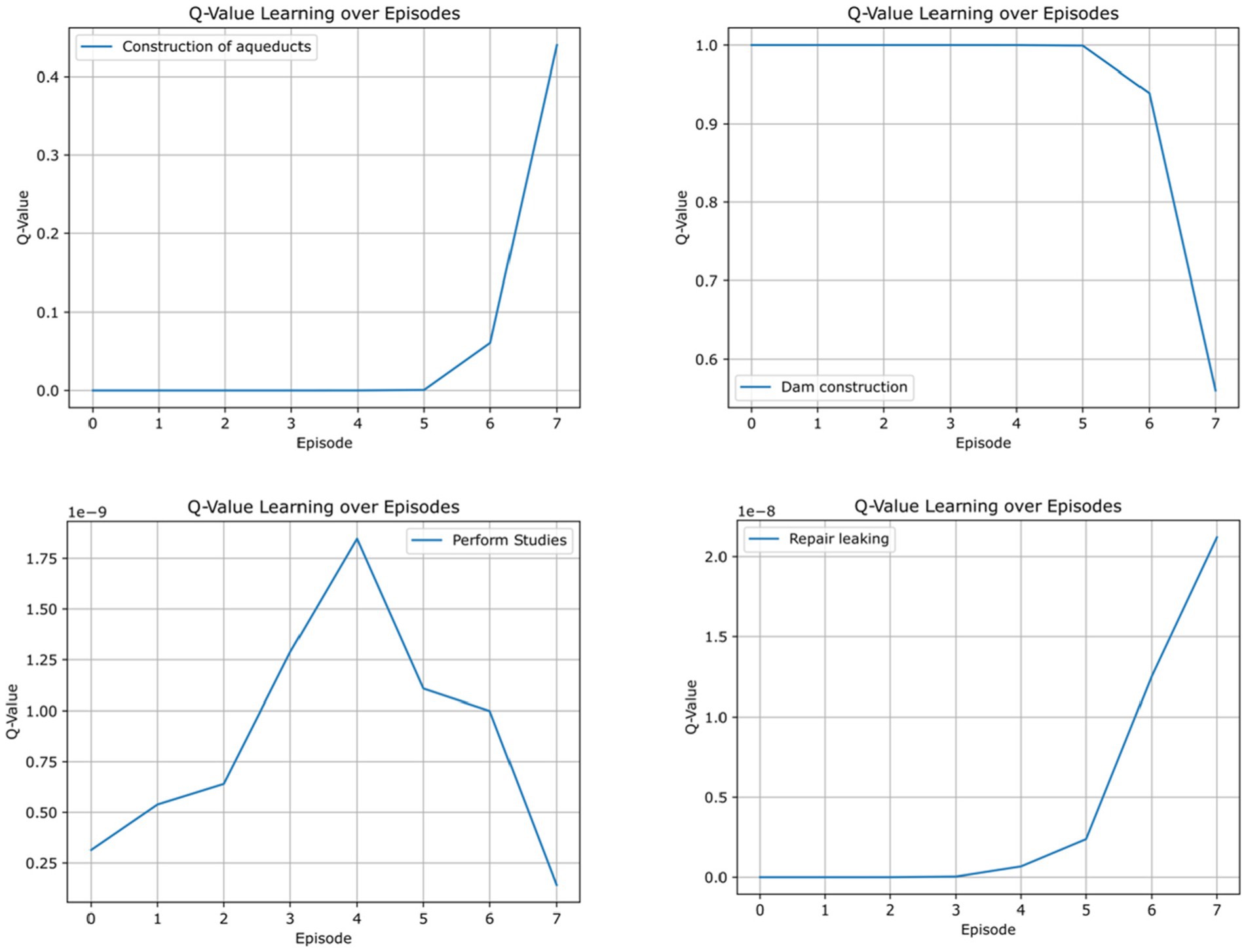
Figure 8. Q-values for different actions.

We note that in all cases, the learning process behaves similarly. First, performing studies is constantly growing as the most important activity until it reaches its highest value, then repair leaking starts. While performing studies is decreasing, it reaches a level where construction of aqueducts begins; this is because the studies are solid enough that modeling the aquifer has reached robust results. Then, the dam construction starts. Note in Figure 8 that dam construction has an opposite trend because it is defined in that way in the reward function construction.

The reward function in RL plays a pivotal role in governing the efficiency and optimization of a process. It essentially serves as the guide that directs an agent toward its goals. This function encapsulates the objectives and priorities of an experienced group, defining what they seek to maximize in their chosen task, thereby shaping the agent’s decision-making to reach those goals.

Designing the reward function in RL is crucial because it guides the learning process, shaping the agent’s behavior to achieve desired goals. However, crafting an effective reward function can be challenging.

Learning can be slow or stall if the agent receives infrequent feedback. Striking the right balance between rare and frequent rewards is essential, so we found that 20 steps is a good balance. We tried exponential and complex linear behavior, but we found that a simple linear combination helps to converge to solutions. Reward engineering requires deep domain knowledge and an understanding of the task. A poorly designed reward function can lead to suboptimal or undesirable agent behavior. Moreover, reconciling conflicting objectives can be tough. Different stakeholders may have different goals, so designing a reward function that balances these objectives is challenging.

A well-designed reward function should also generalize to various situations, allowing the agent to adapt to new scenarios without extensive manual adjustments.

Our example represents one of the different variants of politics that can be implemented. In our case, we have focused on the construction of dams since this corresponds to an immediate need. The phases and actions in the RL process are, therefore, presented only for the purpose of a simple exercise and test. Our computer code is published at https://github.com/rortegaru/DQNWATER.

Once we have implemented the RL process, we can use it for various purposes. The different ways to use this methodology include:

(a) Classification: Benefit serves as a measure to classify the aquifer most beneficial to society’s needs. In our case, the benefit is the reward function when compared to all the different aquifers. (b) Optimal Sequences: Another more traditional approach is to analyze each aquifer separately, attempting to understand the RL learning process. This helps us determine how to apply the relationships between actions and states for each case. (c) Complexity: We can introduce additional elements, like a complex water network system and observe the decision-making behavior. We have provided some examples of these analyses.

7 Application to the Mexican aquifers

According to the World Water Assessment Program (Water, 2012), Mexico is in a region that is quickly approaching absolute physical water scarcity (Figure 9). Climate change, urban growth, and farming needs drive Mexico’s water scarcity. The country’s diverse climates, ranging from arid in the north to humid in the south, make managing water problems difficult. As development increases, so does the pressure on water supplies, raising concerns about ensuring clean water for everyone. This urgent issue challenges policymakers to find ways to save and manage water to avoid a crisis.

Figure 9

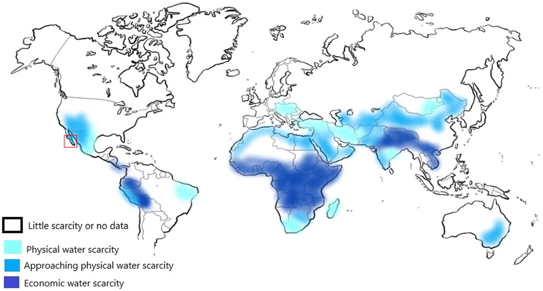
Figure 9. Global map of physical water scarcity. The red square shows the study region [Adapted and modified from World Water Assessment Program (WWAP), March 2012].

Suppose we want to classify the aquifers requiring immediate attention. In that case, we can utilize the entire database of the Federal Commission of Water (CONAGUA, from the Spanish acronym Comisión Nacional del Agua). In Figure 10, we depict the 564 aquifers of Mexico with the four initial states. The Mexican aquifers comprise a combination of the United States Hydrological Unit Codes (HUC) 6 and 8 (Seaber et al., 1987). Data were collected from the repositories of CONAGUA and the Mexican Census 2020 (Instituto Nacional de Estadística, Geografía e Informática, 2020; Comisión Nacional del Agua, 2023). Figure 10 depicts four distinct states for each watershed.

Figure 10

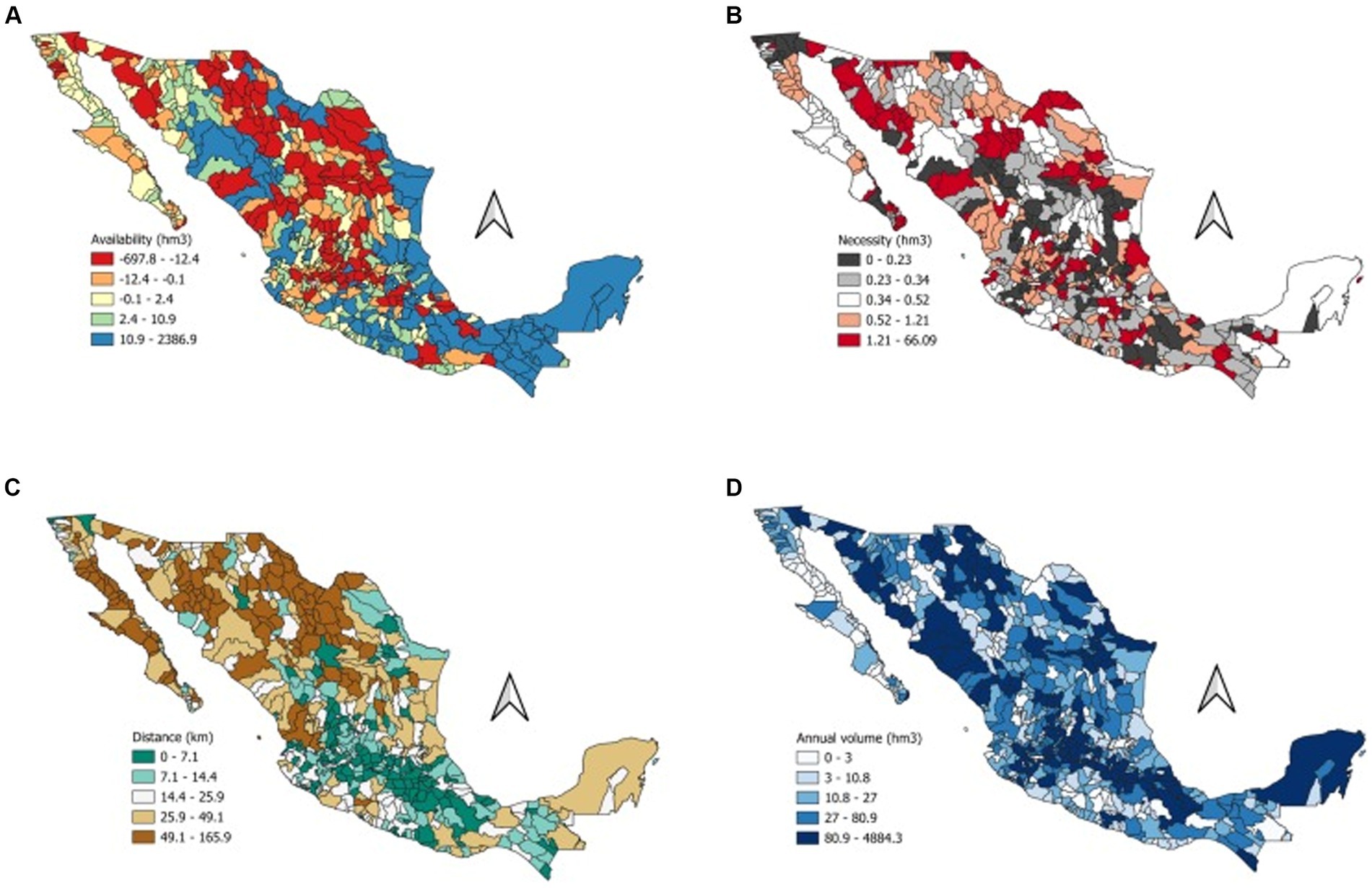
Figure 10. Maps representing the watersheds of Mexico based on four different states. (A) Availability in hectometers, (B) necessity in hectometers. (C) shortest distance to population and (D) Annual volume in hectometers.

Next, we selected only deficit watersheds (Figure 11). Notably, desert and highland regions are in deficit, while the northern part of the country faces more significant availability challenges than the southern part. We refer to watersheds in deficit as critical watersheds.

Figure 11

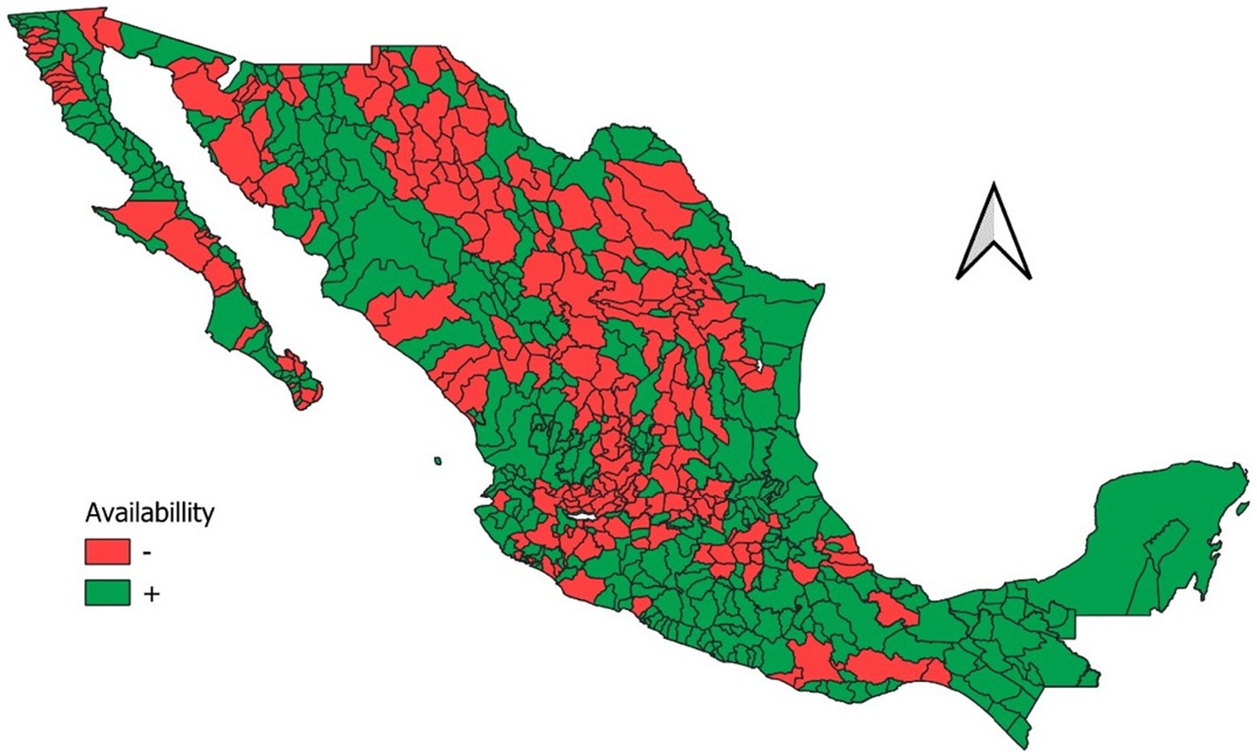
Figure 11. Deficit and available watersheds in Mexico. The watersheds in deficit are used for further analysis in the RL process.

In Figure 12, we compare critical and non-critical watersheds. Based on availability, we display the highest and lowest values for four states in critical watersheds. Out of 653 watersheds, 56 are considered critical due to deficits. In the Electronic Supplement, we present that table. Critical watersheds, accounting for merely 8.6% of the total, span 41% of Mexico’s land area. This emphasizes the crucial importance of studying these critical watersheds. We have excluded modeling values, assuming most studies start from scratch without prior modeling.

Figure 12

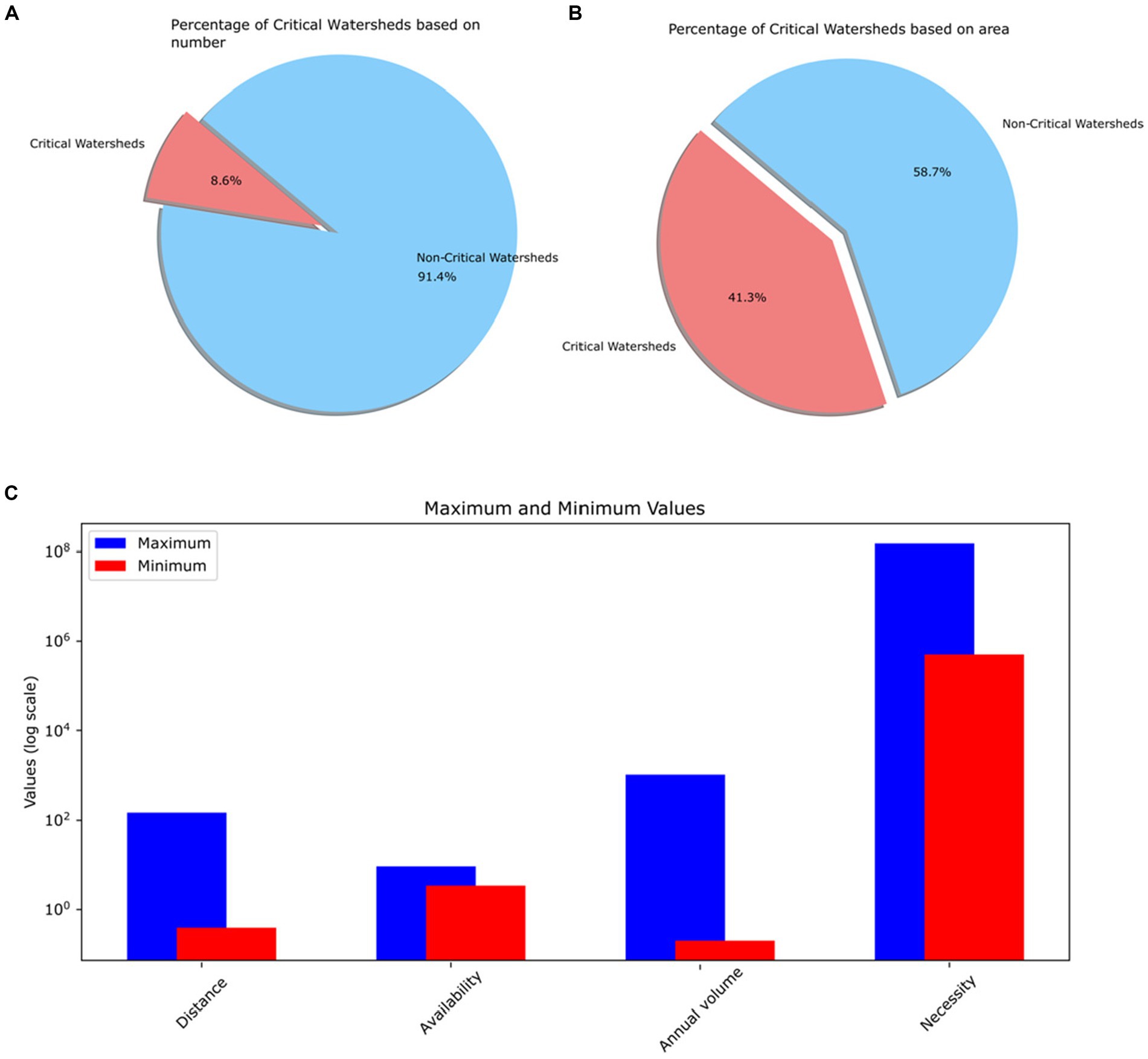
Figure 12. Percentage of critical watersheds: (A) based on numbers, (B) Based on area, (C) Maximum and minimum values of four different states representing critical watersheds.

Next, we evaluated critical watersheds using our RL process and illustrated the benefits in Figure 13. Aquifers with the highest benefit scores receive the highest reward function values. This includes aquifers that are in proximity, have nearby populations, are in critical condition, and can address issues through water infrastructure repairs.

Figure 13

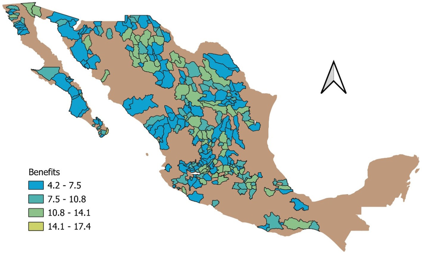
Figure 13. Watersheds with highest benefits.

Finally, we analyzed only the watersheds of Baja California Sur. In Figure 14, we show the watersheds in a similar way to what we presented in Mexico. According to the latest available data, Baja California Sur stands out as the state with the highest water stress levels in Mexico. This situation mirrors challenges seen in other countries across the American continent, such as Chile. Addressing the pressing issues in Baja California Sur is crucial. However, it is essential to note that while this case highlights a significant concern; our approach should not be overly generalized. Instead, we should tailor our strategies and actions to the specific circumstances of each case. By maintaining a critical perspective and focusing on localized solutions, we can effectively address water stress issues and inform targeted public policies.

Figure 14

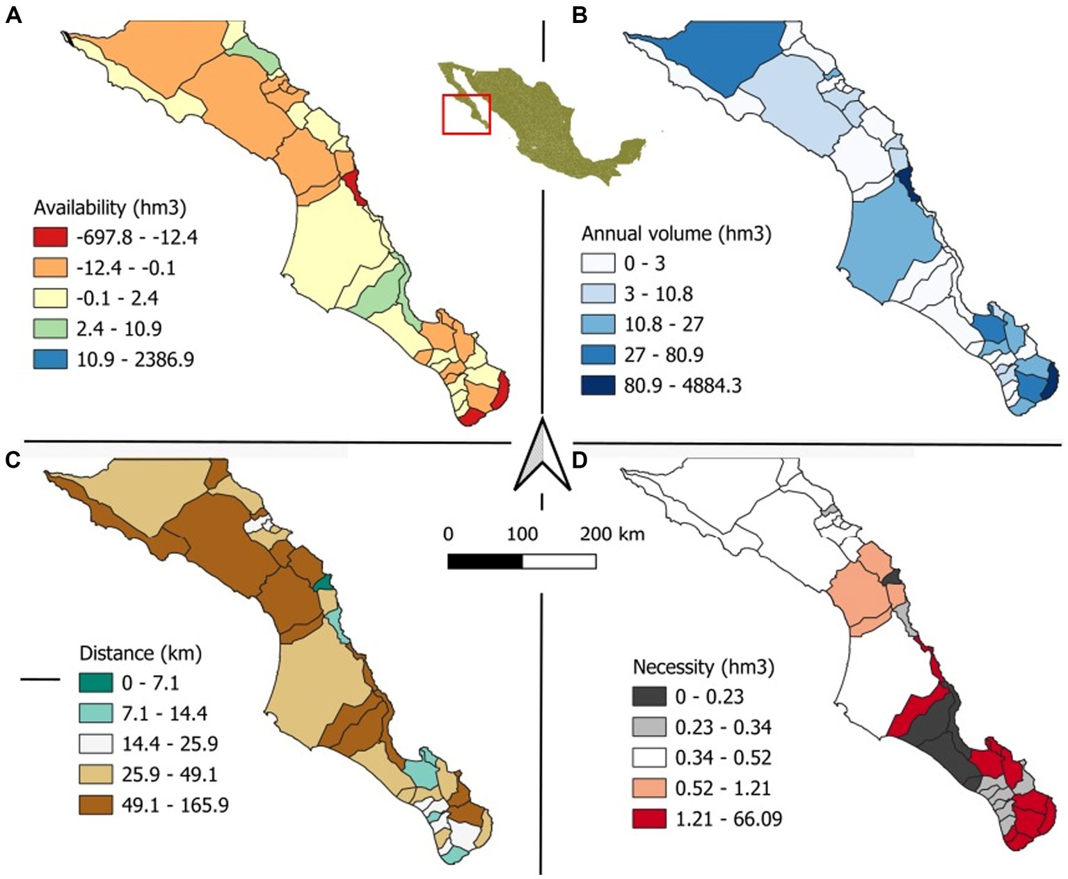
Figure 14. Maps of Baja California Sur based on four different states. (A) Availability in hectometers, (B) annual volume in hectometers, (C) shortest distance to population, and (D) necessity in hectometers.

In this case, we proceeded in the same way as we did in the entire country; however, we added a simple simulation that includes a “repair leaking” based on the distribution of the streets in the major cities of Baja California Sur. Instead of using a simple percentage of 30% (Jornada, 2023), we used the number of streets and buildings and performed our steps based on that number. In Figure 15, we show the water network that we constructed to simulate that number.

Figure 15

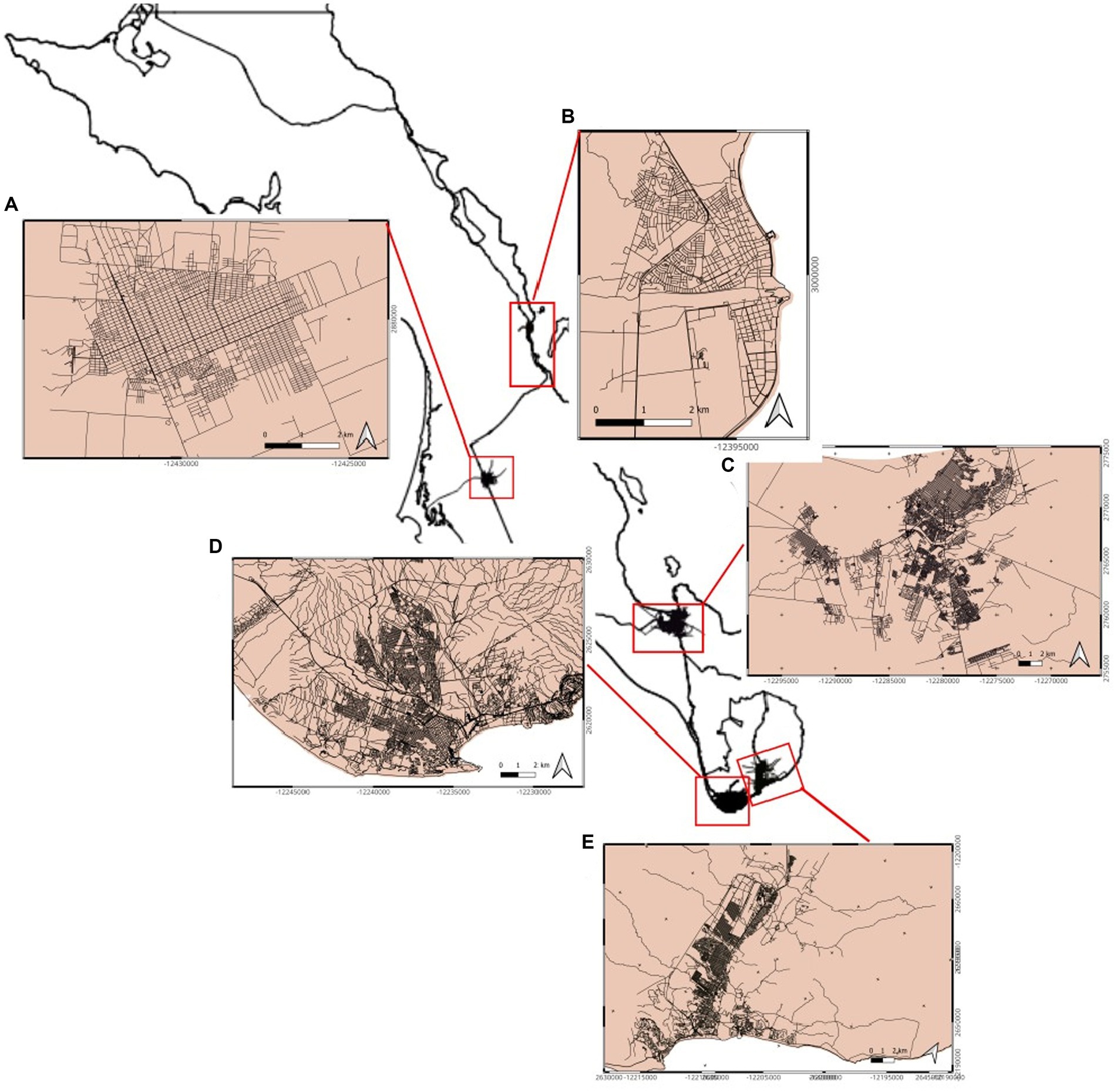
Figure 15. Water grids of the five cities with population higher to 10,000 habitants. (A) Cd. Constitución, (B) Loreto, (C) La Paz, (D) Cabo San Lucas, and (E) San José del Cabo.

In Figure 16 and Table 1, our results reveal a complex trade-off among the states and actions defining the final benefit value. Notably, proximity to population centers and needs plays a crucial role in hierarchical definitions. Consequently, as requested by the Mexican Consejo Nacional de Humanidades, Ciencias y Tecnologías (CONAHCYT) in the 10-year project Researchers for Mexico, we have successfully derived an unbiased value to prioritize the study of watersheds, considering social, technical, and beneficial aspects. Following our analysis, we recommend prioritizing the study of four watersheds (Todos Santos, Melitón Albañez, Cañada Honda, and Plutarco Elias Calles) due to their highest benefit scores.

Figure 16

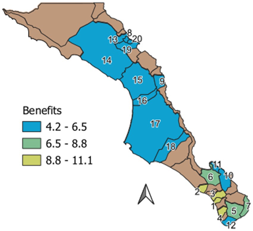
Figure 16. Benefit map of Baja California Sur. All the numbered watersheds are in a deficit state. The assessment of benefits is quantified using the reward function. Watersheds correspond to Table 1.

Table 1

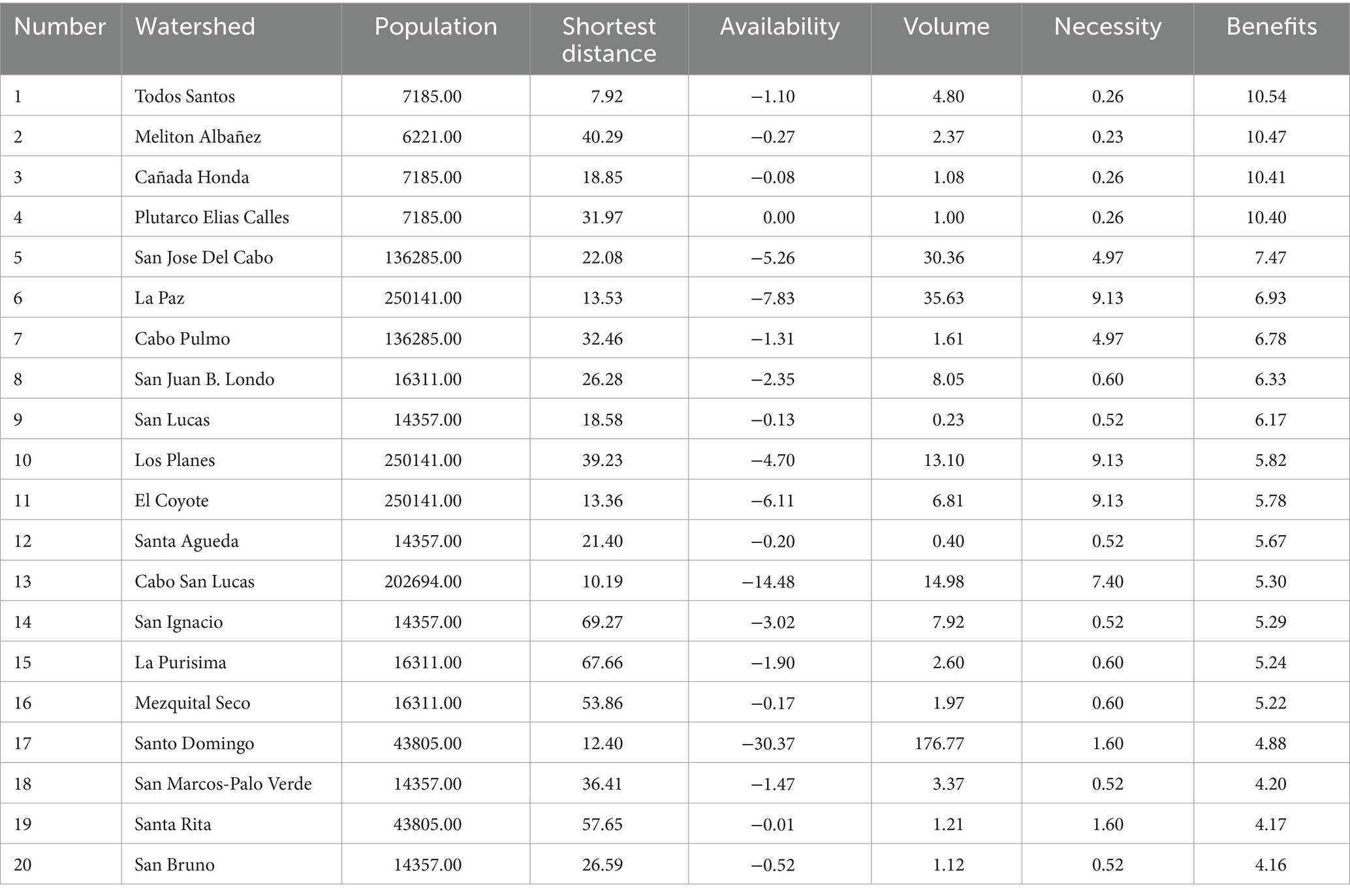
Table 1. Benefit value defined a complex trade-off among the states and actions.

8 Discussion

It is necessary to have an intrinsic connection between states and actions in the RL framework for water management Annual Volume, Necessity, Availability, Distance and Modeling are crucially linked with actions such as Repair leaking, Construction of aqueducts, Dam construction, and Perform studies, requiring a tailored approach to address specific aspects of water management. The success of water management depends more on the specific model we create than on the RL technique itself. Although RL is used for optimization, the real challenge is building a model that accurately represents water management issues through its states and actions. Essentially, how well RL works depends on how good the model is, making the model’s design crucial for addressing real-world problems.

This integrated setup underscores RL’s unique capability to guide learning processes toward making informed decisions, distinguishing it from other machine learning methods that might prioritize accuracy without steering the learning. RL’s adaptability and iterative nature, guided by continuous feedback, enable dynamic strategy updates, starkly contrasting conventional supervised learning paradigms. Our exploration further delves into the practical application within a simulated water management system, emphasizing the role of a carefully designed reward function and the challenge of balancing complex state-actions relationships to foster efficient learning and decision-making.

Our findings highlight the delicate balance between exploration and exploitation in the RL process, where the agent progressively refines its strategy to achieve greater rewards. However, this aspect of learning is not the most critical component because, ultimately, the key factor is the score of the reward function. Even if learning becomes stagnant, it is essential to continually evaluate the reward function, as its performance is the ultimate measure of success in this context. In some cases, having a robust evaluation metric, such as the score of the reward function, is more important than the specific steps taken to reach the optimal decision.

The finite-infinite time horizon problem deals with limiting the number of steps; using a high number of steps, say 10,000, is a useful practice in certain cases. However, limiting the number of steps can be problematic because we do not know if the goal will be reached. Therefore, waiting for the RL to reach its final target is better. For this reason, we have not limited the number of steps; instead, we have carefully revised the penalty rules so that it will always reach its target, no matter if it is thousands of steps. Remember that the optimization mechanism will oversee finding the best solution.

Calibrating the hyperparameters (ε, η) is a work in progress and is currently out of our reach. An example is the discount factor η (Equation 1), which balances the previous rewards with the current one. A low value favors the immediate rewards, while a high value favors the long-term values; that is, it controls the “memory” of the rewards of each state. Although we have decided to use high values to give weight to all the values using a factor that allows us to remember the previous states, a detailed study is necessary to find the optimal value.

Reinforcement learning offers a multitude of advantageous facets beyond mere optimization in complex systems like water management. Its adaptability allows it to tackle unforeseen challenges and dynamic changes within an environment, making it an invaluable tool for long-term planning and decision-making. Moreover, RL’s ability to learn from interactions and feedback enables the development of strategies that improve over time, thereby enhancing efficiency and effectiveness in achieving goals. This iterative learning process, grounded in trial and error, fosters innovation by encouraging the exploration of new solutions. Furthermore, RL’s versatility extends its applicability across various domains, from robotics and automation to healthcare and finance, demonstrating its potential to provide tailored, impactful solutions in diverse settings.

Our study demonstrates how RL can effectively address key water management challenges, as shown in our analysis of Mexican aquifers and the distinction between critical and non-critical watersheds. By using RL to assess watersheds for potential benefits, we gain a deeper understanding of these complex issues. Our findings lead to recommending specific watersheds for focused study, considering their impact on society, technology, and benefits to guide future water management strategies.

Traditional water management methods, such as the Analytic Hierarchy Process (AHP) and others, have offered structured frameworks to address complex decision-making by deconstructing problems into more straightforward, hierarchical elements. These methods stress systematic analysis and prioritization grounded in expert judgment and pairwise comparisons, enabling a more deterministic approach to decision-making. While effective for static and well-defined problems, these conventional methods may lack the flexibility and adaptability to confront dynamic environmental conditions and evolving water management challenges. Their dependence on predefined criteria and expert input can also constrain their capacity to assimilate new data and adapt to unforeseen water availability or demand changes.

In contrast, RL presents a more dynamic and adaptive approach to water management, capable of continuously learning from the environment and optimizing decisions based on real-time feedback. Unlike methods such as AHP, RL algorithms can navigate complex and uncertain environments through trial and error, adjusting strategies based on outcomes and rewards. This capacity for learning and adaptation renders RL particularly suited for the complexities of water management, where conditions can swiftly change due to climatic variability, population growth, and shifting land use patterns. RL’s potential to derive optimal strategies through iterative learning and its ability to handle high-dimensional data and uncertainty positions it as a promising tool for innovative water management solutions, marking a significant advancement over traditional methods.

In addition to the AHP, traditional water management has depended on methods such as Cost–Benefit Analysis (CBA), Linear Programming (LP), and Multi-Criteria Decision Making (MCDM). CBA evaluates the financial aspects of water projects by comparing costs and benefits, focusing on economic efficiency. LP addresses water resource allocation problems through mathematical optimization, striving for the optimal outcome within specified constraints. MCDM, akin to AHP, considers various factors and stakeholder preferences to inform decision-making, providing a systematic approach to assessing intricate scenarios.

Reinforcement learning represents a departure from these traditional methods by adopting a dynamic, feedback-oriented approach. Unlike the static, often linear frameworks of CBA, LP, and MCDM, RL excels in environments characterized by incomplete information and fluctuating conditions. It learns optimal actions through trial and error, guided by a reward system aligned with water management goals. This adaptability enables RL to address real-world complexities, such as sudden water availability or demand patterns, rendering it a versatile tool for contemporary water management challenges. While traditional methods offer valuable insights through structured analysis, RL’s capacity for continuous learning and adaptation presents a forward-looking approach to managing water resources in an increasingly uncertain world.

This study marks a pioneering effort in Mexico, particularly within Baja California Sur, by concentrating on watershed management for public use. While previous research (Mendoza et al., 1997) on climate change and urban studies (Cotler et al., 2022) has primarily focused on ecosystems and sustainability, our work stands out by applying RL to watershed management. This innovative approach represents a growing trend globally in leveraging advanced computational techniques for environmental management. Notably, to our knowledge, this is the first work employing a rule-based RL strategy specifically tailored for watershed management, introducing a novel perspective to the field and potentially setting a precedent for future studies. We show a global tendency toward water management and machine learning, including the paradigm of RL in a more graphical way using bibliometric analysis (Figure 17).

Figure 17

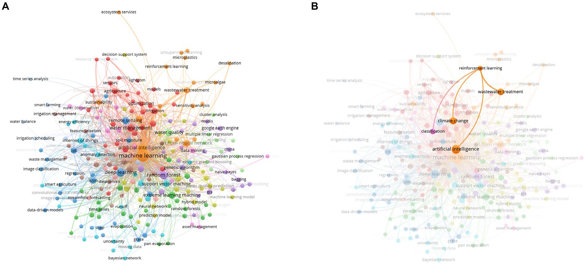
Figure 17. Bibliometric analysis of papers on machine learning and water management from 2020 to 2024. (A) General overview and (B) RL enhancement. The RL paradigm is still in its nascent stage.

In practical terms, implementing RL in water management requires the involvement of stakeholders who can influence activities and outcomes. Boards of directors and governing bodies should take part in formulating strategies and actions, while experts design initial prototypes and establish the groundwork for the relationships between actions and states. These experts should also contribute to defining the reward function, as it will be the basis for optimization.

For instance, if we aim to optimize the design and installation of desalination plants using RL, essential factors such as: energy requirements (in MWatts), intake water quality (measured by total dissolved solids), discharge rate (in l/s), etc., should be identified as states. Discussions should then focus on determining appropriate reward functions and considering initial states. An optimization analysis can show the relationships between states and actions, leading to decisions like placing absorption wells or choosing between direct intake or well-intake methods.

9 Conclusion

We have developed an RL with the ruled-based system to generate a process that defines optimal decision values over time. This process allows us to choose the best actions based on different states within a complex aquifer system, where we have integrated physical characteristics and changes in social and human factors within an artificial intelligence framework. The most important conclusions of this work are as follows:

a. Integrating rule-based actions to achieve optimal decisions in water management needs specific goals that are not universally applicable.

b. Classifying critical watersheds is an effective process for RL.

c. RL tackles the complex connections among its constituent elements.

Our research field opens new avenues for the definition of reward functions and state-change algorithms to improve continuously. Future research should explore integrating rule-based actions alongside RL to refine decision-making for specific objectives, like identifying watersheds that significantly benefit society, especially in mountainous and arid regions that remain a priority. This entails a deeper analysis of the intricate relationships within these ecosystems and the urgent need for interventions in areas facing acute water scarcity.

In summary, this approach to water management and decision-making policies forms part of an intricate decision network that can expand over time.

Data availability statement

The datasets presented in this study can be found in online repositories. The names of the repository/repositories and accession number(s) can be found in the article/Supplementary material.

Author contributions

RO: Writing – original draft, Writing – review & editing. DC: Writing – original draft, Writing – review & editing. AC-M: Writing – review & editing.

Funding

The author(s) declare that financial support was received for the research, authorship, and/or publication of this article. The financial support for this research was provided through the grants CF–2023-G-958 and 319664 from CONAHCYT, and the “Investigadores por México” Project 1220 and CICESE Internal projects 691-106 and 691-118.

Acknowledgments

We extend our deepest gratitude to the two reviewers whose invaluable insights and suggestions have significantly broadened and enriched the scope of our work. Their expertise has enhanced the quality of our research and inspired us to explore our topic from a more comprehensive perspective. The authors acknowledge the authorities of the State Water Commission of Baja California Sur, the National Water Commission, and the municipality of La Paz, including its operating organization, for their valuable recommendations and feedback.

Conflict of interest

The authors declare that the research was conducted in the absence of any commercial or financial relationships that could be construed as a potential conflict of interest.

Publisher’s note

All claims expressed in this article are solely those of the authors and do not necessarily represent those of their affiliated organizations, or those of the publisher, the editors and the reviewers. Any product that may be evaluated in this article, or claim that may be made by its manufacturer, is not guaranteed or endorsed by the publisher.

Supplementary material

The Supplementary material for this article can be found online at: https://www.frontiersin.org/articles/10.3389/frwa.2024.1384595/full#supplementary-material

References

Abadi, M., Barham, P., Chen, J., Chen, Z., Davis, A., Dean, J., et al. (2016). TensorFlow: a system for large-scale machine learning. In 12th USENIX symposium on operating systems design and implementation (OSDI 16). Available at: https://www.usenix.org/conference/osdi16 (Accessed July 12, 2023).

Google Scholar

Amasyali, K., Munk, J., Kurte, K., Kuruganti, T., and Zandi, H. (2021). Deep reinforcement learning for autonomous water heater control. Buildings 11:2023. doi: 10.3390/buildings11110548

Crossref Full Text | Google Scholar

Bellman, R. (1957). A Markovian decision process. J. Math. Mech. 6, 679–684.

Google Scholar

Binas, J., Luginbuehl, L., and Bengio, Y. (2019). Reinforcement learning for sustainable agriculture. ICML 2019 Workshop Climate. Available at: https://www.climatechange.ai/papers/icml2019/32 (Accessed July 22, 2023).

Google Scholar

Brockman, G., Cheung, V., Pettersson, L., Schneider, J., Schulman, J., Tang, J., et al. (2016). Openai gym. arXiv [Preprint]. Available at: https://arxiv.org/abs/1606.01540 (Accessed July 22, 2023).

Google Scholar

Castelletti, A., Galelli, S., Restelli, M., and Soncini-Sessa, R. (2010). Tree-based reinforcement learning for optimal water reservoir operation. Water Resour. Res. 46, 1–19. doi: 10.1029/2009WR008898

Crossref Full Text | Google Scholar

Chen, X., and Ray, A. (2022). Deep reinforcement learning control of a boiling Water reactor. IEEE Trans. Nucl. Sci. 69, 1820–1832. doi: 10.1109/TNS.2022.3187662

Crossref Full Text | Google Scholar

Chen, K., Wang, H., Valverde-Pérez, B., Zhai, S., Vezzaro, L., and Wang, A. (2021). Optimal control towards sustainable wastewater treatment plants based on multi-agent reinforcement learning. Chemosphere 279:130498. doi: 10.1016/j.chemosphere.2021.130498

PubMed Abstract | Crossref Full Text | Google Scholar

Chichilnisky, G., and Heal, G. (1993). Global Environmental Risks. J. Econ. Perspect. 7, 65–86. doi: 10.1257/jep.7.4.65

Crossref Full Text | Google Scholar

Comisión Nacional del Agua. (2023). Disponibilidad de acuíferos. Available at: https://sigagis.conagua.gob.mx/gas1/sections/Disponibilidad_Acuiferos.html (Accessed January 10, 2024).

Google Scholar

Cotler, H., Cuevas, M., and Landa, R. (2022). Environmental governance in urban watersheds: the role of civil society organizations in Mexico. Sustain. For. 14, 1–988. doi: 10.3390/su14020988

Crossref Full Text | Google Scholar

Emamjomehzadeh, O., Kerachian, R., Emami-Skardi, M. J., and Momeni, M. (2023). Combining urban metabolism and reinforcement learning concepts for sustainable water resources management: a nexus approach. J. Environ. Manag. 329:117046. doi: 10.1016/j.jenvman.2022.117046

PubMed Abstract | Crossref Full Text | Google Scholar

Ghobadi, F., and Kang, D. (2023). Application of machine learning in Water resources management: a systematic literature review. Water 15, 1–620. doi: 10.3390/w15040620

Crossref Full Text | Google Scholar

Gorelick, S. M., and Zheng, C. (2015). Global change and the groundwater management challenge. Water Resour. Res. 51, 3031–3051. doi: 10.1002/2014wr016825

Crossref Full Text | Google Scholar

Hu, C., Cai, J., Zeng, D., Yan, X., Gong, W., and Wang, L. (2020). Deep reinforcement learning based valve scheduling for pollution isolation in water distribution network. Math. Biosci. Eng. 17, 105–121. doi: 10.3934/mbe.2020006

PubMed Abstract | Crossref Full Text | Google Scholar

Hu, X., Chu, L., Pei, J., Liu, W., and Bian, J. (2021). Model complexity of deep learning: a survey. Knowl. Inf. Syst. 63, 2585–2619. doi: 10.1007/s10115-021-01605-0

Crossref Full Text | Google Scholar

Hu, C., Wang, Q., Gong, W., and Yan, X. (2022). Multi-objective deep reinforcement learning for emergency scheduling in a water distribution network. Memet Comput 14, 211–223. doi: 10.1007/s12293-022-00366-9

Crossref Full Text | Google Scholar

Huang, W.-Y., and Uri, D. N. (1990). Optimal policies for protecting the quality of groundwater. Resour. Energy 11, 371–394. doi: 10.1016/0165-0572(90)90005-4

Crossref Full Text | Google Scholar

Instituto Nacional de Estadística, Geografía e Informática. (2020). Censo de Población y Vivienda 2020. Available at: https://www.inegi.org.mx/programas/ccpv/2020/ (Accessed January 10, 2024).

Google Scholar

Ingold, K., and Tosun, J. (2020). Special issue “public policy analysis of integrated water resource management.”. Water 12, 1–2321. doi: 10.3390/W12092321

Crossref Full Text | Google Scholar

Jornada, L. (2023). Se desperdicia por fugas entre 20 y 60%de agua potable en varios estados. Available at: https://www.jornada.com.mx/notas/2022/04/30/estados/se-desperdicia-por-fugas-entre-20-y-60-de-agua-potable-en-varios-estados/ (Accessed January 10, 2024).

Google Scholar

Khampuengson, T., and Wang, W. (2022). Deep reinforcement learning ensemble for detecting anomaly in telemetry water level data. Water 14, 1–2492. doi: 10.3390/w14162492

Crossref Full Text | Google Scholar

Lee, K. M., Ganapathi Subramanian, S., and Crowley, M. (2022). Investigation of independent reinforcement learning algorithms in multi-agent environments. Front. Artif. Intellig. 5:805823. doi: 10.3389/frai.2022.805823

PubMed Abstract | Crossref Full Text | Google Scholar

Mendoza, V., Villanueva, E., and Adem, J. (1997). Vulnerability of basins and watersheds in Mexico to global climate change. Clim. Res. 9, 139–145. doi: 10.3354/cr009139

Crossref Full Text | Google Scholar

Mohtadi, H. (1996). Environment, growth, and optimal policy design. J. Public Econ. 63, 119–140. doi: 10.1016/0047-2727(95)01562-0

Crossref Full Text | Google Scholar

Ortega, R. (2024). DQN WATER. Available at: https://github.com/rortegaru/DQNWATER (Accessed January 10, 2018).

Google Scholar

Ramos, H. M., McNabola, A., López-Jiménez, P. A., and Pérez-Sánchez, M. (2020). Smart water management towards future water sustainable networks. Water 12, 1–58. doi: 10.3390/w12010058

Crossref Full Text | Google Scholar

Ruelens, F., Claessens, B. J., Quaiyum, S., De Schutter, B., Babuška, R., and Belmans, R. (2018). Reinforcement learning applied to an electric Water heater: from theory to practice. IEEE Trans. Smart Grid 9, 3792–3800. doi: 10.1109/TSG.2016.2640184

Crossref Full Text | Google Scholar

Santoro, A., Frankland, P. W., and Richards, B. A. (2016). Memory transformation enhances reinforcement learning in dynamic environments. J. Neurosci. 36, 12228–12242. doi: 10.1523/JNEUROSCI.0763-16.2016

PubMed Abstract | Crossref Full Text | Google Scholar

Savenije, H. H. G., and Van Der Zaag, P. (2005). “Integrated water resources management concepts and issues” in 31st IAHR Congress 2005: Water Engineering for the Future, Choices and Challenges.

Google Scholar

Seaber, P. R., Kapinos, F. P., and Knapp, G. L. (1987). Hydrologic unit maps: US Geological Survey water supply paper 2294. US Geological Survey. Available at: https://pubs.usgs.gov/wsp/wsp2294/pdf/wsp_2294.pdf (Accessed January 10, 2024).

Google Scholar

Sivamayil, K., Rajasekar, E., Aljafari, B., Nikolovski, S., Vairavasundaram, S., and Vairavasundaram, I. (2023). A systematic study on reinforcement learning based applications. Energies 16, 1–1512. doi: 10.3390/en16031512

Crossref Full Text | Google Scholar

Skirzyński, J., Becker, F., and Lieder, F. (2021). Automatic discovery of interpretable planning strategies. Mach. Learn. 110, 2641–2683. doi: 10.1007/s10994-021-05963-2

Crossref Full Text | Google Scholar

Strnad, F. M., Barfuss, W., Donges, J. F., and Heitzig, J. (2019). Deep reinforcement learning in world-earth system models to discover sustainable management strategies. Chaos 29:123122. doi: 10.1063/1.5124673

PubMed Abstract | Crossref Full Text | Google Scholar

Water, U. N. (2012). World Water Assessment Programme. Water in a Changing World: Facts and Figures. Paris: Unesco

Google Scholar