From global glacier modeling to catchment hydrology: bridging the gap with the WaSiM-OGGM coupling scheme

Coupled glacio-hydrological models have recently become a valuable method for predicting the hydrological response of catchments in mountainous regions under a changing climate. While hydrological models focus mostly on processes of the non-glacierized part of the catchment with a relatively simple glacier representation, the latest generation of standalone (global) glacier models tend to describe glacier processes more accurately by using new global datasets and explicitly modeling ice-flow dynamics. Yet, to the authors' knowledge, existing catchment-scale coupled glacio-hydrological models either do not include these most recent advances in glacier modeling or are simply not available to other users. By making use of the capabilities of the free, distributed, physically-based Water Flow and Balance Simulation Model (WaSiM) and the Open Global Glacier Model (OGGM), a coupling scheme is developed to bridge the gap between global glacier representation and local catchment hydrology. The WaSiM-OGGM coupling scheme is used to further assess the impacts under future climates on the glaciological and hydrological processes in the Gepatschalm catchment (Austria), by considering a combination of three climate projections under the Representative Concentration Pathways (RCP) 2.6, 4.5, and 8.5. Additionally, the results are compared to the original WaSiM model with the integrated Volume-Area (VA) scaling approach for modeling glaciers. Although both models (WaSiM with VA scaling and WaSiM-OGGM coupling scheme) perform very similar during the historical simulations (1971–2010), large discrepancies arise when looking into the future (2011–2100). In terms of runoff, the VA scaling model suggests a reduction of the mean monthly peak between 10–19%, whereas a reduction of 26–41% is computed by the coupling scheme. Similarly, results suggest that glaciers will continuously retreat until 2100. By the end of the century, between 20–43% of the 2010 glacier area will remain according to the VA scaling model, but only 1–23% is expected to remain with the coupling scheme. The results from the WaSiM-OGGM coupling scheme raises awareness of including more sophisticated glacier evolution models when performing hydrological simulations at the catchment scale in the future. As the WaSiM-OGGM coupling scheme is released as open-source software, it is accessible to any interested modeler with limited or even no glacier knowledge.

1 Introduction

In high mountainous regions, which are characterized by large precipitation sums and low temperatures, glaciers play a fundamental role. They act as huge reservoirs of fresh water and are therefore a crucial component in the water balance cycle (Meier, 1969; Ersi et al., 2009). During winter, water is stored and subsequently released during warmer months when ice and snow melt, contributing to the generation of runoff. Even small glacierized headwaters within larger river basins can significantly contribute to runoff downstream, and therefore impact the reliability of water supply (Huss, 2011). This effect is particularly noticeable in water-stressed regions. This is because the largest contribution of meltwater occurs in summer, when groundwater contribution, and in some regions precipitation, are often at their lowest (e.g., Cochand et al., 2019; Schaffer et al., 2019). In a warming climate, glacier contribution to runoff will change. Accelerating melt rates will lead to a decrease in glacier volume and increased runoff, causing the peak discharge to shift to spring or early summer (Koboltschnig and Schöner, 2011; Marzeion et al., 2012; Hanzer et al., 2018). The contribution of glacier melt to the runoff will gradually decline over a prolonged period due to the reduction in glacier volume (Huss et al., 2008; Naz et al., 2014), as is expected for the European Alps, for example. Here, strong warming conditions could result in a reduction of around 90% of the current glacier volume by the end of the century (Zekollari et al., 2019). Similar losses are expected to occur in water-scarce regions, for example in Himalayan basins (Wood et al., 2020; Dixit et al., 2021). The implications in these regions could be extremely serious, as glaciers are a reliable source of domestic water supply for many communities.

To better understand and predict the evolution of glaciers and their contribution to runoff in mountain hydrology, glacio-hydrological models are a powerful tool. They combine catchment hydrology and glacier modeling to offer a comprehensive representation of all the processes involved (Stoll et al., 2020; van Tiel et al., 2020). However, modeling glaciers remains a challenging issue, especially due to scarce long-term glaciological measurements (i.e., mass balances, Naz et al., 2014). Moreover, numerous models rely on empirical methods to estimate glacier evolution, such as the Volume-Area (VA) scaling approach (Bahr et al., 1997, 2015) or the Δh method (Huss et al., 2010). Although the first method can provide reliable estimates of glacier volume (e.g., Radić et al., 2007; Kormann et al., 2016), and the second can accurately attribute the effect of changes in glacier geometry to runoff trends (e.g., Duethmann et al., 2015), an explicit representation of the ice-flow dynamics is missing.

In this context, great progress has been made in coupling standalone glacier models to hydrological models, with the aim of improving the representation of glaciers and their contribution to runoff. For example, Stoll et al. (2020) applied two independent glacio-hydrological models, HQsim-GEM and AMUNDSEN, and compared future changes in the glaciology and hydrology of an Austrian catchment. While HQsim-GEM is a combination of the hydrological model HQsim and the glacier evolution model GEM, AMUNDSEN is a hydroclimatological model that implements the Δh method for modeling glacier geometries. In addition, AMUNDSEN, which was originally developed by Strasser et al. (2008), was successfully used to assess future climate change impacts on the hydrology of the Ötztal Alps (Hanzer et al., 2016, 2018). Other examples can be found in Stahl et al. (2008) and Naz et al. (2014). In the first study, a semi-distributed conceptual hydrological model HBV-EC model was coupled to a glacier response model, in which glacier evolution is considered through the VA scaling approach. In the second study, the authors coupled the hydrological soil-vegetation model DHSVM to the Glacier Dynamics Model GDM to predict the future effect of glacier recession on streamflow in a Canadian catchment.

While it is widely acknowledged that glacier retreat and subsequent mass loss on a global scale play a significant role in both sea-level-rise and regional runoff, it is only in recent years that extensive research has been conducted on the subject of global glacier studies (Radić and Hock, 2014; Huss and Hock, 2015). The available global Randolph Glacier Inventory (RGI, RGI Consortium, 2017) together with glacier mass changes observations (e.g., Zemp et al., 2019; Hugonnet et al., 2021) around the globe, have been proving to be a valuable resource in taking global glacier modeling a step further. These achievements can clearly be seen through some state-of-the-art models, such as the Global Glacier Evolution Model (GloGEM, Huss and Hock, 2015), the Open Global Glacier Model (OGGM, Maussion et al., 2019), and the Python Glacier Evolution Model (PyGEM, Rounce et al., 2020). In the field of hydrology, Wiersma et al. (2022) already exploited the capabilities of the GloGEM model by coupling it to the PCR-GLOBWB 2 global hydrological model. In their study, they highlight the added value of using a global glacier model for better representing glacier evolution and hence the runoff predictions in highly glacierized catchments. Yet, the coupling scheme developed focuses on large-scale basins. Besides, the glacier model still relies on the empirical Δh method and is only available upon request. Another example can be found in Khadka et al. (2020), where the Open Global Glacier Model (OGGM) is integrated into the Glacio-hydrological Degree-Day Model (GDM). The coupled model is then used to predict the future response of a Himalayan catchment until 2100. However, the independent models are not driven with exactly the same input climate data.

Although more coupled glacio-hydrological models have become available recently, not all are freely accessible to the user. Furthermore, most models still rely on empirical routines to estimate glacier evolution, thereby missing the explicit ice-flow dynamics that can be supplied by most global models. In order to bridge the gap between glacier representation and the hydrological response of a catchment, we developed a coupling scheme in which we combined a distributed, process-based hydrological model with a global glacier model for the Gepatschalm catchment in Austria. To achieve our purpose, we used OGGM (Maussion et al., 2019) to produce annual glacier outputs based on explicit ice-flow dynamics and subsequently coupled it to the Water Flow and Balance Simulation Model (WaSiM, Schulla, 1997). Since WaSiM represents non-glacier (and even glacier) processes with notable success (e.g., Verbunt et al., 2003; Kormann et al., 2016; Thornton et al., 2021), we rely on WaSiM for simulating non-glacier processes (e.g., evapotranspiration) and replace the integrated VA scaling approach by OGGM's outputs. Compared to Khadka et al. (2020), the WaSiM-OGGM coupling scheme shows more consistency in terms of feedback between independent models, as both WaSiM and OGGM are driven with the same input climate dataset. Furthermore, it extends the common procedure of only transferring one output variable from one model to the other (e.g., glacier areas only, as suggested by Khadka et al., 2020 and Stoll et al., 2020, or glacier runoff only, like Wiersma et al., 2022 did), since the feedback between models includes glacier areas, ice thickness distributions, and glacier mass balances. Additionally, we applied the coupling scheme to predict the glacio-hydrological response of the catchment under future climate conditions and compared the results to the VA scaling approach. This WaSiM-OGGM coupling scheme may serve as an open-source tool for improving runoff predictions in high mountainous catchments and for policy making in water resources management.

2 Materials and methods

2.1 Study area and data

The Gepatschalm area is located in the Kaunertal region, in the Ötztal Alps (Austria), and covers a total surface of 57.5 km². Figure 1A shows the location of the study area within Austria and Figure 1B the topography, where elevations of around 1,880 m a.s.l. can be found near the gauging station and elevations up to ~3,500 m a.s.l. can be found in the southern boundaries, near the glaciers. Moreover, the observed glaciers outlines for 1969 (Patzelt, 2013) and 2015 (Buckel and Otto, 2018) are included in the figure, showing a clear reduction in glacierized area in recent decades. In 1969, 47% of the study area was covered by glaciers, and by 2015 this reduced to 36%. The climate in the region is mostly warm and dry (Hanzer et al., 2018), where the mean annual total precipitation recorded by two nearby stations (2,640 and 1915 m a.s.l.) was 700 mm for the period 1990–1997. The mean annual temperature for the same period was −1.2 °C.

Figure 1

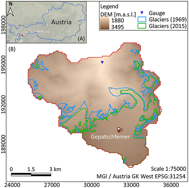
Figure 1. (A) Location of study area within Austria, (B) topography, glacier outlines for the years 1969 and 2015 (Patzelt, 2013; Buckel and Otto, 2018) and location of the gauging station with available runoff measurements.

2.1.1 Climate data

Within and around the study area (up to ~30 km away) more than 50 stations have been measuring hourly and daily values of precipitation (P), temperature (T), relative humidity (RH), wind speed (WS), and global radiation (GR). However, only a few stations cover all variables and for a period long enough for the simulations. To apply the WaSiM-OGGM coupling scheme, all variables need to be known for each model grid cell. This can be achieved using analysis or re-analysis datasets with high spatio-temporal resolution. For example, the Austrian Meteorological Service (Zentralanstalt für Meteorologie und Geodynamik, ZAMG) offers a multivariable analysis and nowcasting system, Integrated Nowcasting through Comprehensive Analysis system (INCA, Haiden et al., 2011), in which numerical weather predictors are combined with real-time observations (station and radar data) and high-resolution topographic data to produce gridded datasets of variables (e.g., P, T, RH, WS, GR). The INCA dataset has been successfully used in the past for hydrological modeling (e.g., Schöber et al., 2010; Förster et al., 2018) and this is used here as a climate input. The spatial resolution of this dataset is 1 × 1 km, whereas the variables are provided with a 1-h time step (except precipitation, which is available at a 15-min resolution). Because the period covered by INCA spans from 2003 to 2019, an analogous downscaling method is adopted to extend the dataset into the past (back to the year 1969). To this end, a kNN (k-Nearest Neighbor, Lall and Sharma, 1996; Winter et al., 2019) re-sampling method is applied. The period 1969–2003 is reconstructed by resampling (with replacement) from nearest neighbors (NN). The new time series is created while preserving statistical properties of the known time series, such as monthly mean temperatures or monthly precipitation sums. NN refers to the days for which the station data from 2003-2019 are closest, with respect to temperature and precipitation patterns, to days within the same month in the kNN-time series (1969–2003). The NN with, for example, the smallest Euclidean distance is subsequently selected as the match-day.

2.1.2 Future projections

To predict the catchment's response and evaluate the performance of the models under future climate projections, high-resolution regional climate model data provided by the EURO-CORDEX initiative (Jacob et al., 2013) is used. The regional climate model data has a horizontal resolution of 0.11 degrees and three different climate model combinations were selected. These are composed of three Global Climate Models (GCM) and three Regional Climate Models (RCM) under different Representative Concentration Pathways (RCP 2.6, 4.5, and 8.5), which are summarized in Table 1. The reference period is taken from 01/1971 to 12/2000 and the data was bias adjusted following the MultI-scale bias AdjuStment (MidAS) tool (v0.2.1.), developed by Berg et al. (2022).

Table 1

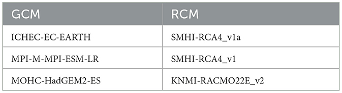
Table 1. GCMs and RCMs considered for the prediction of the catchment's response in the future.

2.1.3 Observed glaciological and hydrological data

Daily measurements of runoff are available at the outlet of the catchment (Figure 1), for the period 01/1985 to 12/2019 [Tiroler Wasserkraft AG (TIWAG)]. Glacier outlines from the Austrian Glacier Inventory are accessible for the years 1969, 1998, 2006, and 2015 (Patzelt, 2013; Fischer et al., 2015; Buckel and Otto, 2018). Furthermore, two types of glacier mass balance datasets are available: (a) average annual geodetic mass balance observations for the period 2000–2020 on a per glacier basis (Hugonnet et al., 2021) and (b) annual glacier mass balance observations at the tongue of Gepatschferner at different elevation heights (from 2,175 to 2,875 m a.s.l.), for the period 2012–2020 (Stocker-Waldhuber, 2019).

2.1.4 Simulation period

The simulation period is split into two parts: (a) the historical period, spanning from 1971 to 2010, and (b) the future period, from 2011 to 2100 (Figure 2). For the historical period, the models are calibrated against available observed data and INCA is used as input climate data. The models are initialized in 1969, since glacier outlines are available for that year. For the future period, the calibrated models are then run for each of the climate projections. Although the future simulations start in 2011, the historical simulations are carried out until the year 2019. This is because that glacier mass balance observations are available mostly only after 2010, thus the glacier model can only be calibrated for that period. Note that the climate projection's historical period ends in 2005 after which the RCPs start. Thus, the last 5 years of the historical period in the hydrological simulations are affected by the RCPs.

Figure 2

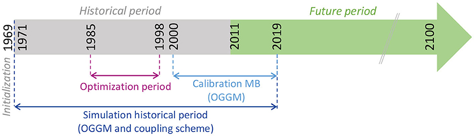
Figure 2. Simulation period. Historical period from 1971 to 2010 and future period from 2011 to 2100. The models are initialized in 1969. The coupling scheme is optimized during the period 1985 to 1998 and the mass balance model in OGGM is calibrated during the period 2000–2019.

2.2 Water balance model including VA scaling

The simulation of the water balance components of the Gepatschalm catchment is performed with the Water Flow and Balance Simulation Model WaSiM (Schulla, 1997, 2021). For this study, the Richards version 10.06.04 (2021) for Windows is used. Table 2 summarizes the main sub-processes considered within WaSiM with their corresponding model or approach. In this study, the main focus is given to the glacier model, which is described in the following section. A detailed description of the remaining sub-processes can be found in the model documentation (Schulla, 2021).

Table 2

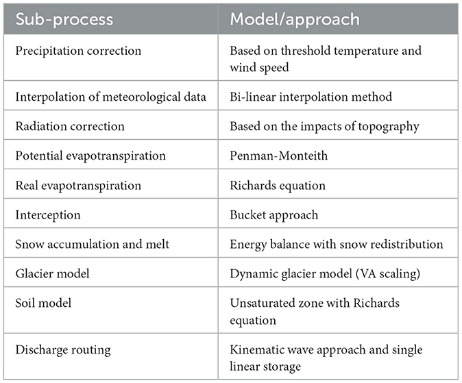
Table 2. Summary of the main sub-processes included in WaSiM.

2.2.1 VA scaling approach

WaSiM simulates glacier evolution with the Volume-area scaling approach, which is based on the physically validated but still empirical relationship described by Equation (1) (Chen and Ohmura, 1990; Bahr et al., 1997):

$\begin{array}{ll}V=b\times A^f& (1)\end{array}$

Where: V is the volume of the glacier (m km²), A is the area of the glacier (km²), b is an empirical scaling factor that represents the mean ice thickness (m) of a 1 km² glacier (default value = 28.5 m) and f is the scaling exponent (−) (default value = 1.36). The default values adopted here correspond to the values suggested by WaSiM, according to the relationship found by Chen and Ohmura (1990) for 63 mountain Alpine glaciers. The VA scaling approach essentially tries to express a volume (V) (L³) by knowing the glacier area (A) (L²). In order maintain consistent units, the units of the scaling factor are usually (L^{3 − 2f}). However, in Equation (1), b is used, since the scaling factor can be intuitively interpreted as the glacier's mean ice thickness per unit area (Grinsted, 2013). To initialize the model, only the glacier area is required, hence no information about the glacier thickness or volume is provided. At the beginning of the simulation, WaSiM determines the initial volume of the glacier based on the area and the VA scaling equation (Equation 1). Thus, it is important to initialize the model in a year with available glacier observations (in this case, the year 1969 is selected). At the end of the first mass balance year (in the Northern Hemisphere, the mass balance year spans from 1st October to 30th September), the glacier's mass balance is converted into a volume by taking into account the ice density. Considering that V_old is the volume of the glacier at the beginning of the mass balance year and V_new is the newly calculated volume at the end of the first year of the simulation, the latter can be expressed as:

$\begin{array}{ll}{V}_{new}=V_{old}+\frac{M{B}_{new}}{{\rho }_{ice}}\times ic{e}_{value}\times cel{l}_{size}& (2)\end{array}$

Where: V_new is the new calculated volume (m km²), V_old is the initial volume of the glacier (m km²), MB_new is the new mass balance rate of the glacier at the end of the mass balance year (mm w.e.) or (kg m⁻²) (Equation 3), ρ_ice is the ice density (kg m⁻³), ice_value is the number of cells identified as glacierized cells and cell_size is the size of the one model cell (km²) (here 100 × 100 m). The mass balance rate gives the change in the mass of a glacier through accumulation (gained mass) and ablation (lost mass). The accumulation is the result of solid precipitation and the internal metamorphosis of snow to firn and then to ice. On the contrary, the ablation refers to the melt rate of the glacier and is described by a temperature-index model (T-index, with or without radiation, Hock, 1999).

$\begin{array}{l}M{B}_{new}=P_{solid}\\ -\left\{\begin{array}{c}(MF+{\alpha }_{ice/firn/snow}\times I_0\times \frac{G_s}{I_s})\times (T-T_0)T>T_0\\ 0T\le T_0\end{array}\right\}& (3)\end{array}$

Where: MB_new is the mass balance rate (mm d⁻¹) from Equation (2), P_solid refers to the solid precipitation (and internal metamorphosis from snow to ice), MF is the melt factor (mm °C⁻¹ d⁻¹), α are empirical coefficients (mm °C⁻¹ d⁻¹), I₀ and I_s are the potential direct incoming shortwave radiation at each grid cell and at defined locations of meteorological stations, respectively (Wh m⁻²), G_s is the observed radiation at the same station (Wh m⁻²), T is the air temperature (°C) and T₀ is the threshold temperature for melt (°C). Then, with the new volume (Equation 2), the new area of the glacier after the end of the mass balance year can be obtained by means of Equation (4):

$\begin{array}{ll}{A}_{new}={(\frac{V_{new}}{b})}^{\frac{1}{f}}& (4)\end{array}$

With the new glacier area A_new, WaSiM estimates the number of cells that need to be added or subtracted (in case the mass balance is positive or negative, respectively) based on an iterative process. This process is done by dividing the glacier into elevation bands of equal elevation differences (Schulla, 2021).

2.3 WaSiM-OGGM coupling scheme

Even though the VA scaling approach is widely used and has demonstrated its efficacy in estimating glacier evolution (e.g., Radić et al., 2007; Stahl et al., 2008), a representation of the explicit ice-flow dynamics is still an open point. In this context, the Open Global Glacier Model OGGM (Maussion et al., 2019) allows modeling the evolution of glaciers by applying a depth-integrated flowline model, in which the ice flux along each of the glaciers' flowlines is computed. Thus, the main idea behind the coupling scheme is to benefit from both models' capabilities and complement their strengths in order to overcome the main challenges that each of them may present:

• WaSiM is a fully-distributed model, whereas OGGM is based on a “1.5D” flowline geometry.

• Daily simulations can be performed with WaSiM, whereas monthly to annual scales are considered in OGGM.

• While in WaSiM the glacier's volume is unknown, OGGM can offer the volume, areas and ice thickness along the flowlines for each glacier.

• OGGM models the glacier's evolution using explicit ice-flow dynamics, whereas WaSiM is based on the empirical VA scaling approach.

The main workflow of the coupling scheme consists of three steps and is depicted in Figure 3. In this study, an “offline” coupling between both models is performed. This means that the models are run separately but the inputs are updated in accordance to the other model's outputs.

Figure 3

Figure 3. Detailed workflow of the coupling scheme with multi-criteria optimization.

2.3.1 First WaSiM run with re-sampling of climate data

To ensure a consistent exchange of variables between the independent models, WaSiM and OGGM are driven with the same climate data. In the first step of the coupling scheme, WaSiM runs on a daily time step. First, precipitation values are corrected, for example, due to wind undercatch (Hanzer et al., 2016). Second, all climate variables (e.g., from the INCA dataset) are bi-linearly interpolated to match the grid cell resolution of the model (from 1 to 0.01 km² in this case). Finally, as OGGM requires monthly input data of temperature and precipitation, these two variables are re-sampled at a monthly time step. Both monthly mean temperature and monthly precipitation sum are calculated from daily timesteps. At this stage, it is important to highlight that this WaSiM run solely serves to prepare the driven climate data for later use by OGGM. However, as this study additionally aims to investigate the differences between the WaSiM-OGGM coupling scheme and the original WaSiM model with VA scaling, the daily outputs (e.g., runoff) are stored and analyzed later in the results section.

2.3.2 OGGM run and processing of glacier outputs

During this step, a dynamic run is carried out in OGGM, using the climate data which was processed and re-sampled to monthly values by WaSiM. By default, OGGM uses the Randolph Glacier Inventory (RGI RGI Consortium, 2017) as initial outlines for the glaciers, which for this case correspond to the year 2003. Since the simulations are conducted from 1969 onwards, the model requires a dynamic spin-up for initialization. During this spin-up, the model tries to find a past glacier state whose area matches that of the glacier outline date by adjusting a temperature bias. The mass balance components are determined by a temperature-index method (Equation 5, Maussion et al., 2023) similar to WaSiM but calibrated on geodetic mass balance observations:

$\begin{array}{ll}{B}_i(z)=P_i^{solid}(z)-d_f\times max(T_i(z)-T_{melt},0)& (5)\end{array}$

Where: B_i(z) is the monthly mass balance rate at elevation z (mm w.e. month⁻¹), $P_i^{solid}(z)$ is the monthly solid precipitation at elevation z (mm month⁻¹), T_i(z) is the monthly temperature at elevation z (°C), T_melt is the temperature threshold at which melt occurs (°C), and d_f indicates the temperature sensitivity of the glacier (mm month⁻¹ °C⁻¹).

The calibration is carried out based on the average annual geodetic mass balance observations for the period 01/2000 to 01/2020 (Hugonnet et al., 2021), in which three parameters (melt factor, temperature bias, and precipitation factor) are adjusted on a per glacier basis. Moreover, to limit the number of calibrated parameters, mass balance observations at Gepatschferner glacier tongue are used as an additional dataset. This prevents an overparameterization of the model, and enables a comprehension of the interannual variability of the mass balance components. Such a model evaluation cannot be achieved solely by comparing the model performance against the average delta in geodetic mass balance observations.

OGGM determines the ice thickness of the glacier based on a flowline model (Maussion et al., 2019, 2023). This means that the ice flows solely along the flowlines, for which the cross-section or bed-shape is defined. As a result, a “1.5D” geometry of the glacier is obtained. This is, however, not sufficient for integrating OGGM's output into WaSiM's simulations, since WaSiM is a fully-distributed model with a 2D computational domain. For this reason, a conversion of the flowline model with “1.5D” geometry into a grid (2D geometry) containing the glacier's outline is carried out. This process is merely based on a geometric approximation whereby the outer points that define the widths of the cross-sections along the flowlines are connected to delineate a plausible glacier outline. The procedure is exemplified in Supplementary Figure S1. Furthermore, an approximation of the ice thickness distribution throughout each glacier and for each year is computed. This allows not only the areas of OGGM to be integrated, but also the glacier volumes, so that explicit representation of the ice dynamics occurs within the coupling scheme. This spatially explicit volume transfer extends the HQsim-GEM approach proposed by Stoll et al. (2020), which has been constructed using only an area feedback between glacier evolution and the hydrological model.

2.3.3 Final WaSiM run: coupling scheme

During the last step of the coupling scheme, the outputs generated from OGGM serve as input when re-running WaSiM. In this step, WaSiM's simulations are still carried out with a daily resolution but the glacier input grids (areas and volumes) are updated on an annual basis. This annual update scheme is justified for several reasons. First, it adheres to the VA scaling approach, as the new glacier volume is estimated at the end of the mass balance year. Second, an annual update of glacier states is a common procedure in comparable studies (e.g., Stoll et al., 2020). Third, the prediction of glacier evolution generally relies on seasonal (e.g., 6-month) to multi-annual scales (e.g., Chiarle et al., 2020), mainly associated with the rather slow glacier's movement, which might only be visible after a year (or several years).

Still, both models calculate the glacier mass balance rates separately, requiring a direct correspondence between them to ensure the proper transfer of the glacier's dynamics from OGGM to WaSiM. In this sense, one obvious solution might be the direct integration of OGGM mass balances into WaSiM, hence substituting the daily mass balance values calculated by WaSiM. However, this cannot be easily achieved and a modification of the model's source code is required. In some cases, the codes are not readily available for the user, or even if they are, a code's modification might work for the current WaSiM's version, but incompatibilities can be expected if another updated version is selected. Besides, in this study, WaSiM is chosen as the hydrological model, but the developed coupling might serve as a basis for coupling OGGM with any other similar model. Moreover, the potential of getting daily mass balance values would be unexploited and this is one of the main capabilities of WaSiM and a primary reason for selecting this model. Consequently, another solution consists of using the glacier mass balance rates calculated by OGGM as a constraint when re-running WaSiM. This is introduced through a multi-criteria optimization approach, in which the most sensitive parameters in WaSiM are automatically adjusted by minimizing the differences between OGGM (assumed to be ‘observed' in this case) and WaSiM (simulated) mass balances rates. To achieve this, the Statistical Parameter Optimization Tool for Python (SPOTPY, Houska et al., 2015) in combination with the Shuffled Complex Evolution algorithm - University of Arizona (SCE-UA, Duan et al., 1994) is used. Since the parameters of the hydrological model need to be calibrated in any case, it is performed only once during the third step of the coupling scheme, thus ensuring the consistency between both independent models as one component of the objective function.

Furthermore, comparisons are made between observed and simulated runoff at the catchment outlet. As a result, the multi-objective function is represented by Equation (6):

$\begin{array}{ll}OF=w_1·(1-KG{E}_Q)+w_2·(1-B{E}_Q)+w_3·abs(BIA{S}_Q)+w_4·RS{R}_{GMB}& (6)\end{array}$

Where: KGE_Q is the Kling-Gupta Efficiency (Gupta et al., 2009), BE_Q is the Benchmark Efficiency (Schaefli and Gupta, 2007) and BIAS_Q is the bias (according to Gupta et al., 1998), all of them calculated based on observed and simulated runoff. RSR_GMB is the Root Mean Squared Error standard deviation ratio between observed and simulated glacier mass balances (Moriasi et al., 2007). w₁ to w₄ are the weights used to assign the magnitude of the contribution of each performance measure into the total objective function. The sum of all weights is equal to 1 and similarly to the study carried out by Tarasova et al. (2016), values of 0.23, 0.4, 0.07, and 0.3 for w₁, w₂, w₃ and w₄ are adopted, respectively. w₁, w₂ and w₃ make the multi-objective function more sensitive to runoff behavior, representing 70% of the total weight. On the other hand, w₄ suggests that glacier mass balance represents a 30% of the total weight in the multi-objective function. This value is in the same order of magnitude to the contribution of ice melt to the total runoff and similar to the value suggested by Tarasova et al. (2016). As depicted in Figure 2, the optimization is carried out for the period 1985–1998, being the model initialized in 1969. Although the maximum number of iterations was set at 3,000, the minimum objective function was found after only 1,218 iterations. The SCE-UA algorithm was employed due to its popularity among hydrological models (van Tiel et al., 2020), but it might be computationally more expensive than other options. Nonetheless, due to the high flexibility of SPOTPY, alternative algorithms and objective functions may be considered. The coupling scheme aims to be a versatile tool that can be tailored to meet the requirements of any modeler.

3 Results and discussion

This section includes the simulation results after running the models for the historical and future periods. The results are presented and analyzed in terms of runoff, glacier mass balances rates and changes in glacierization (volumes and areas). The focus is given to the comparison between the results of the water balance model with the integrated VA scaling approach (for simplification, here named VA scaling) and the WaSiM-OGGM coupling scheme (simply referred as the coupling scheme).

A brief discussion on the results of the coupling scheme optimization is addressed first. As stated in Section 2.3.3, the multi-objective function OF (Equation 6) consists of several functions that may have varying magnitudes, causing challenges in weight assignment. However, upon completion of the optimization procedure, it becomes evident that all values fall within a similar range. More specifically, the values of the involved objective functions are shown by replacing the values in Equation (6):

$\begin{array}{l}OF=0.23·(1-0.88)+0.4·(1-0.25)+0.07·abs(0.061)\\ +0.3·0.72=0.55& (7)\end{array}$

These findings underscore the general applicability of this user-defined OF.

3.1 Runoff

3.1.1 Historical period

Figure 4 shows the simulation results during the historical period (1971–2010). The simulated runoff is the result of the two different models: VA scaling and the coupling scheme. Moreover, the figure includes the observed runoff and the performance measures of each model (observed vs. simulated values). Since the observed runoff is available only after 01/1985, the performance measures refer to the period 01/1985 to 12/2010. In both models, the simulated runoff is underestimated during spring/summer and slightly overestimated during autumn. Since snow melt is the primary contributor to runoff during spring, the underestimation might be attributed to the snow model. In both cases, VA scaling and coupling scheme, the melting from snow is described using an energy balance approach that also considers gravitational slides and wind redistribution. However, snow melt on glaciers is described differently, following the T-index approach (similar to Equation 3). Even though WaSiM offers the possibility to model snow melt on glaciers using the same approaches selected within the snow model, the simulation results showed more deficiencies and was therefore not considered.¹ On the other hand, the overestimation of autumn runoff could be due to glacier melt, as this is the main component contributing to runoff during this season.

Figure 4

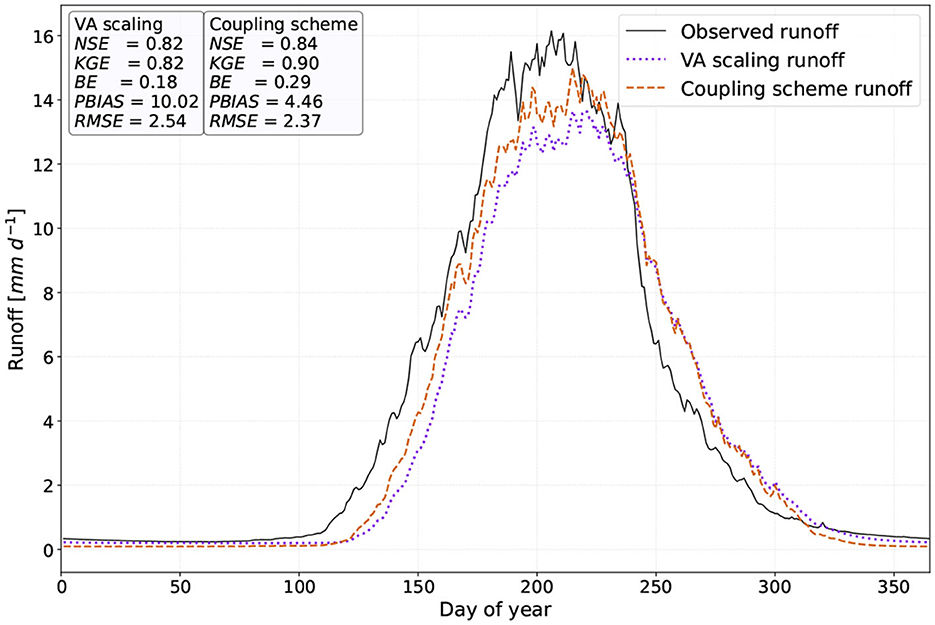
Figure 4. Mean daily observed (black solid line, period 1985–2010) and simulated runoff (violet point line: WaSiM with VA scaling, brown dashed line: WaSiM-OGGM coupling scheme) for the historical period (1971–2010) and corresponding performance measures.

Essentially, both models show a very good performance in simulating runoff, making it challenging to determine which model is more suitable. However, the primary objective of this coupling scheme is not to provide a more accurate representation of runoff, but rather to offer a more robust and reliable model that could potentially improve the simulation results in glacierized catchments in the future. For this reason, the future period is analyzed in the following section.

3.1.2 Future period

Figure 5 shows the mean monthly runoff for the reference and three different future periods (rows, from bottom to top): 1971–2010, 2011–2040, 2041–2070, and 2071–2100. The diagrams on the left are the results of the VA scaling model, whereas the diagrams on the right indicate the results of the coupling scheme. In all diagrams, the results are depicted as an ensemble mean of the three GCM/RCMs combinations and for the three different RCPs (blue for RCP2.6, green for RCP4.5 and red for RCP8.5), with their corresponding spread. The simulated mean monthly runoff for the historical period (1971–2010, black dashed line) is also included.

Figure 5

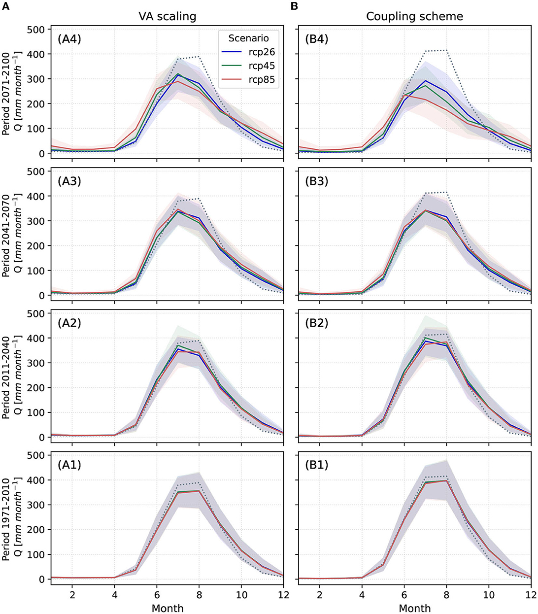
Figure 5. Mean monthly runoff for the reference and three different future periods (rows, from bottom to top: 1971–2010, 2011–2040, 2041–2070, 2071–2100) and for the two models: (A) WaSiM with VA scaling integrated approach and (B) WaSiM-OGGM coupling scheme. The values represent the ensemble mean of the three GCM/RCMs combinations and for RCP2.6 (blue), RCP4.5 (green), and RCP8.5 (red). The black dashed line indicates the simulated mean monthly runoff during the historical period.

During the reference period (first row, 1971–2010), almost no differences can be observed between simulation results. The models behave similarly under the different RCPs and the results are close to the historical simulations. Like the results shown in Figure 4, the VA scaling model seems to slightly underestimate the peak runoff, compared to the coupling scheme. For the near future (period 2011–2040, second row), both models behave similarly and there are only small differences between simulation results under the different RCPs. The mean monthly peak is slightly reduced and remains in August for RCP8.5 for both models but is shifted to July for RCP2.6 and 4.5. Moreover, there is an increase of the winter flows, between September and December. This increase can also be seen when analyzing the middle period 2041–2070 (third row). In addition, for both models and for all RCPs, the mean monthly peak already shifts to July, suggesting that the runoff of the catchment changes from a glacial/glacionival to a nivo-glacial regime (Hanzer et al., 2018). When comparing the results of both models, it is evident that the coupling scheme exhibits a stronger reduction of the monthly peak, while the VA scaling model demonstrates higher runoff values during spring, particularly for RCP8.5.

Comparable results are observed during the last period 2071–2100 (upper row), where the mean monthly peak is reduced and shifted to July. However, the coupling scheme results for RCP8.5 suggest that the peak could shift to June with a stronger reduction in magnitude (44% peak reduction compared to the historical period). Again, simulated winter runoff increases in both models, most importantly for RCP8.5. In spring months, the VA scaling model shows an increase in the monthly values relative to the coupling scheme. The mean annual runoff for RCP8.5 during the latest period is 1,393 mm for the VA scaling and 1,108 mm for the coupling scheme. This suggests that the simulated runoff from the coupling scheme is ~20% lower than the results from the VA scaling, so the increased spring values do not compensate the strong reduction of runoff during summer. Similarly, the coupling scheme yields values that are 8 and 14% lower for RCP2.6 and RCP4.5, respectively.

In addition, Figure 6 shows the 30-year mean annual simulated runoff for the same future periods (columns, left to right: 2011–2040, 2041–2070, and 2071–2100). For each period, the figures indicate the ensemble mean of the GCM/RCMs and are displayed based on the RCPs. Each diagram also features the mean values from the historical period and both models. This figure shifts the focus from the seasonal response of the catchment to the annual totals. In this way, it is possible to infer whether the lower summer values predicted by the coupling scheme might compensate the higher spring values predicted by the VA scaling model, as seen in Figure 5.

Figure 6

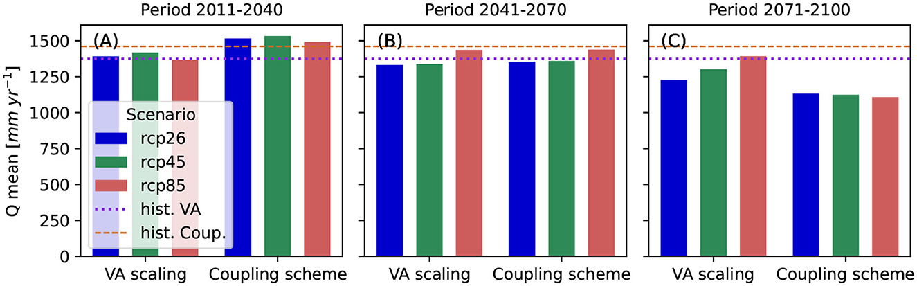
Figure 6. Thirty-year mean annual runoff values as a result from both models, for different future periods: (A) 2011–2040, (B) 2041–2070 and (C) 2071–2100. The values represent the ensemble mean of the three GCM/RCMs combinations, for RCP2.6 (blue), RCP4.5 (green), and RCP8.5 (red). The mean annual historical values for the VA scaling and the coupling scheme are also included in the figure.

When analyzing the first period (2011–2040), results from each individual model indicate minimal changes relative to the historical period. These findings align with the seasonal response depicted in Figure 5, where the VA scaling model also produces slightly lower values. When looking at the second period (2041–2070), although Figure 5 indicates that the peak in summer is reduced in all scenarios and for both models, Figure 6 suggests that the annual amount might increase with the VA scaling model for RCP8.5. On the contrary, the mean annual values are reduced within the coupling scheme for all scenarios, compared to the historical period. Finally, for the third period (2071–2100), the same behavior is expected as for the second period and VA scaling model. Nevertheless, the coupling scheme produces noticeably reduced mean annual runoff values, 26% lower values compared to the historical period and for RCP8.5. In contrast, the VA scaling results predict a potential increase of 2% in mean annual runoff for the same RCP, compared to the historical period.

3.2 Glaciers

To better understand the relatively diverse response between both models when simulating runoff under future climate projections, glacier evolution is analyzed in detail in the next sections.

3.2.1 Glacier mass balance

Figure 7 depicts the annual mass balance rates for all the glaciers within the study area, simulated by both models (VA scaling on the left and coupling scheme on the right) and as a total average for the entire catchment. Glacier mass balance rates for the historical period are indicated in gray until 2011, which denotes the beginning of the future projections. Future projections are represented by the ensemble mean of the three GCM/RCMs combinations together with their respective spread, and for the different RCPs (blue for RCP2.6, green for RCP4.5 and red for RCP8.5).

Figure 7

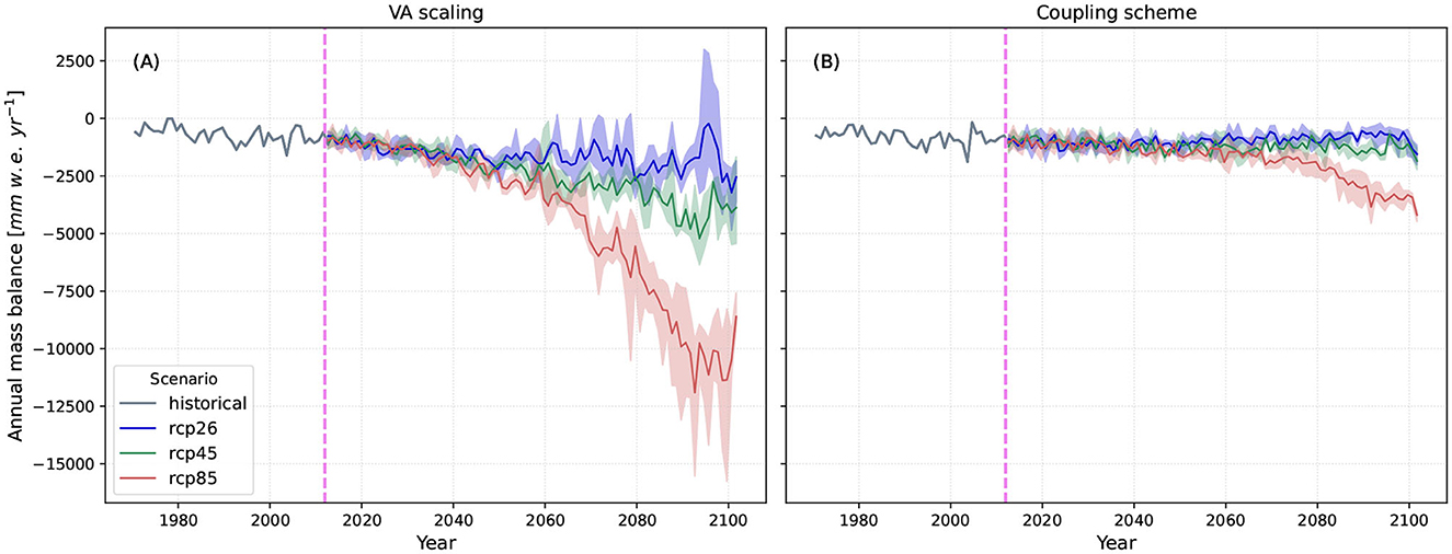
Figure 7. Annual mass balance rates as a total average (mm w.e. yr^-1): (A) WaSiM with VA scaling integrated approach and (B) WaSiM-OGGM coupling scheme. The values represent the ensemble mean of the three GCM/RCMs combinations and for RCP2.6 (blue), RCP4.5 (green), and RCP8.5 (red). The gray line indicates the results during the historical period.

From Figure 7 it is clear that the models exhibit comparable behavior throughout the historical period, with the VA scaling and coupling scheme models yielding a mean annual mass balance rate of −0.71 and −0.82 m w.e., respectively. For RCP2.6, the VA scaling results indicate a significant rise in inter-annual variability. At the end of the century, a total average cumulative mass loss of ~142 m w.e. is expected (this value is obtained through the integration of annual mass balance values over time). On the other hand, the results from the coupling scheme suggests that only 124 m w.e. will be lost by 2100 (thus, the mass loss obtained from the VA scaling is 13% higher than from the coupling scheme). From the simulation results under RCP4.5 and 8.5, higher losses are expected. The total average mass loss at the end of the century under RCP4.5 is ~214 m w.e. for the VA scaling and 144 m w.e. for the coupling scheme. The greatest difference between simulation results, however, is observed under RCP8.5. In this case, according to the VA scaling, the study area could potentially encounter an overall average mass loss of almost 390 m w.e. by 2100, whereas the results from the coupling scheme show almost half of that (198 m w.e.). This rather odd behavior of the VA scaling under RCP8.5 might be attributed to the very small glacierized areas that still prevail in the region at the end of the century. Considering that the mass balance is the change in mass per unit area, even a very small area might lead to huge mass balance rate values.

3.2.2 Glacier volumes and areas

In Figure 8, simulated glacier areas are compared to the observed outlines for the year 1998 (29 years after initialization of the model). On the left, the results from the WaSiM simulations with the integrated VA scaling approach are shown, whereas on the right, the results from the coupling scheme with the areas obtained from OGGM are presented. In both cases, the simulated areas are represented by glacier coverage in each model cell. If a model cell does not contain any glacier, then the value is 0%. On the contrary, if a model cell is completely covered by glaciers, the value reaches 100% and is represented by the dark blue color. Any value between 0 and 100% is depicted with lighter blue colors, as shown in the legend. Furthermore, the evaluation of the simulation results in terms of glacier areas is summarized with two performance measures. On the one hand, the Probability of Detection (POD) indicates the ability of the model to correctly predict glacierized cells. On the other hand, the False Alarm Rate (FAR) indicates that the model simulation identified glacierized cells where no glaciers were observed. Both measures range between 0 and 1, 1 being the optimum value for POD and 0 for FAR (Kormann et al., 2016).

Figure 8

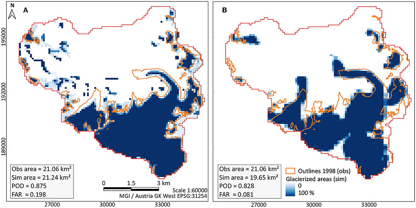
Figure 8. Glacier areas: observed (orange) and simulated glacier areas (blue) for the year 1998. (A) WaSiM with VA scaling integrated approach and (B) WaSiM-OGGM coupling scheme.

While the simulation results from the VA scaling suggest that the model more accurately represents glacier shapes (higher POD), the coupling scheme is less prone to falsely simulate glacierized cells (lower FAR). The generation of false glacierized areas with the VA scaling model might be attributed to the snow model, which enables the re-distribution of snow and therefore the accumulation of it in model cells throughout the years, which will finally lead to the conversion of snow into firn and then into ice. An advantage of the coupling scheme is that, since the glacier areas are updated every year considering the ice-flow dynamics determined by OGGM, unlikely (i.e., “numerical glaciers” Freudiger et al., 2017, which are still viewed as challenging within glacio-hydrological models) accumulation amounts of snow/firn/ice throughout the years are avoided. However, the simulated areas from the coupling scheme exhibit a few deficiencies, which are already evident in Figure 8.

First of all, since the conversion from OGGM's flowline model into a 2D glacier geometry is based on a geometric approximation, the delineation of the glacier shape is not entirely accurate. This is clear, for example, in the southern part of Gepatschferner, where part of the glacier is excluded due to an inaccurate connection of points. Second, the tongue of some glaciers, including Gepatschferner, seem to be rather exaggerated. This outcome is related to the dynamic spin-up of the glaciers and the unknown geometry (or glacier state) considered during the initialization of OGGM. During the dynamic spin-up, an initial state of the glaciers is searched until the simulated areas match the given observed values (i.e., from the RGI date). Therefore, glaciers might grow in the past so that this initial state together with the given historical climatic conditions lead to the presently known geometries. The only drawback is that glaciers can only grow along the flowlines because of OGGM's nature, which in the end results in “longer” glacier tongues. Finally, OGGM is not capable of creating glaciers prior to the RGI's date. For this reason, it is not possible to model glaciers that existed before the RGI's date and have since melted completely or partially persist in the study area.

The evaluation of the models performances in terms of glacierized volumes and areas under future climate conditions is depicted in Figure 9. The upper row refers to the area of the glaciers, whereas the lower row refers to the volume. The left diagrams correspond to the results from the VA scaling model and the right diagrams to the coupling scheme. The historical simulations (1971–2010) are shown in gray. The ensemble mean of the future simulations, which start in the year 2011, are shown for the different RCPs, and the observed areas are indicated for the years 1969, 1998, 2006, and 2015 (red dots).

Figure 9

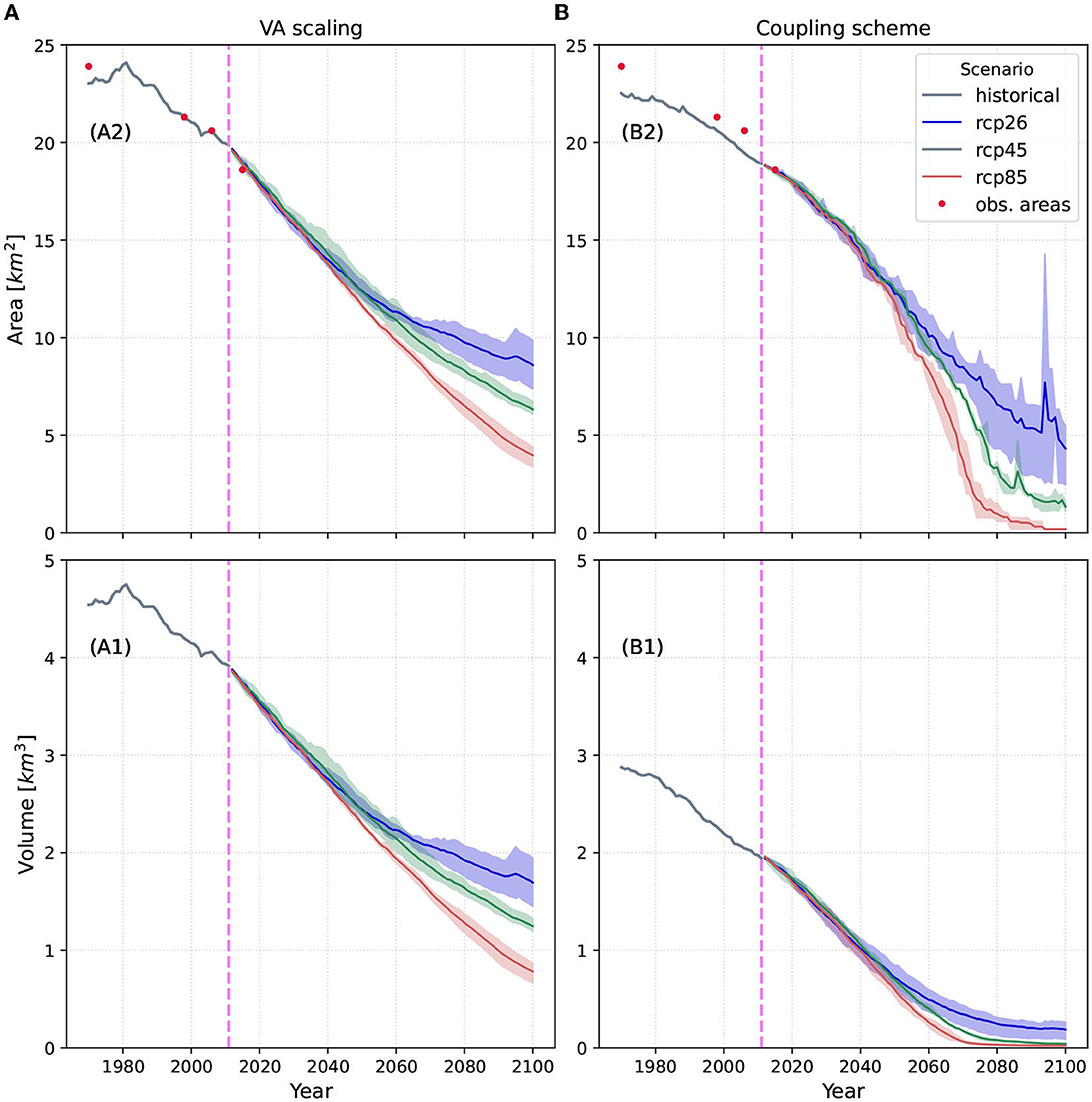
Figure 9. Glacier volumes and areas: (A) WaSiM with VA scaling integrated approach and (B) WaSiM-OGGM coupling scheme. The upper row indicates the glacier areas, whereas the lower row the volumes. The values represent the ensemble mean of the three GCM/RCMs combinations and for RCP2.6 (blue), RCP4.5 (green), and RCP8.5 (red). The gray line indicates the results from the historical simulation and the red dots the observed areas according to the RGI.

When looking at the evolution of the glacier areas throughout the historical period, it becomes clear that both models behave quite similarly. Even though the coupling scheme seems to underestimate the areas in the past, both models reach a similar value by the end of the period. In 2010, the total area simulated by the VA scaling model is 19.9 km², whereas a value of 19.0 km² is obtained from the coupling scheme. This similar behavior between models can still be perceived until 2040 and for all RCPs, where results differ by only 2% (glacier area of 14.0 and 14.3 km² for the VA scaling and coupling scheme, respectively). After 2040, a greater deviation in areas between models is expected. For example, under the VA scaling, the total glacier coverage is expected to reach 8.6 km² by the end of the century for RCP2.6. In contrast, this value is 4.3 km² when considering the coupling scheme. That means that by the year 2100, 77% of the glaciers will melt according to the coupling scheme, but only 57% according to the VA scaling, compared to the areas in 2010. For RCP4.5, the aforementioned values escalate to 93 and 68% respectively, and they become extreme for RCP8.5, where a total area loss of 99 and 80% is expected by the coupling scheme and the VA scaling, respectively.

In terms of volumes, the discrepancies between model results are much larger. On the one hand, the initial volume within WaSiM simulations is determined directly and empirically with the VA scaling equation (Equation 1), where only the glacier area is known. On the other hand, the coupling scheme relies on the volume determined by OGGM, which is based on the ice-flow dynamics and depends on the ice thickness and bed shape of the glacier. Moreover, the annual update of the glacier volumes is performed differently in each model. In the case of WaSiM with VA scaling, the same relation between volume and area is maintained over the years, since the empirical factors affecting Equation (1) remain unchanged. On the contrary, the feedback from OGGM is integrated annually into the coupling scheme, hence, this relation is updated each year and is based on modeled ice-flow dynamics. At the beginning of the simulations, the VA scaling model predicts a total volume of 4.5 km³, equivalent to a mean ice thickness of nearly 80 m distributed throughout the total Gepatschalm area. As for the coupling scheme, this value is 2.9 km³ or 50 m of ice thickness. The initial volume clearly affects the glacier's evolution in the future. With regard to the VA scaling, glacier volumes of 1.7, 1.3, and 0.8 km³ are projected for RCP2.6, 4.5, and 8.5, respectively, by 2100. These values are significantly more optimistic than those predicted by the coupling scheme, where almost all glaciers would have disappeared by the end of the century and under all RCPs (0.19, 0.04, and 0.02 km³ for RCP2.6, 4.5, and 8.5, respectively).

Finally, Figure 10 shows the spatially distributed glacier coverage for the year 2070. The figure contains three main columns that represent the different RCPs and that are divided according to the model (VA scaling and coupling scheme). The rows refer to the GCM/RCMs combinations. As a reference, the observed glacier outlines corresponding to the year 1998 are included in the figure. Similarly to Figure 8, the blue colors indicate the percentage of glacierization in each model cell.

Figure 10

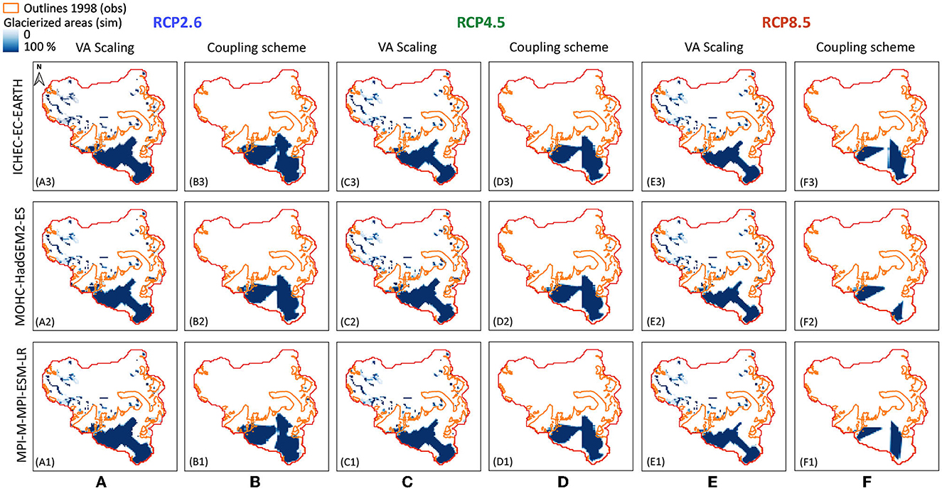
Figure 10. Projected glacier coverage for the year 2070, under the three different RCPs: (A) VA scaling and (B) coupling scheme, both under RCP2.6, (C) VA scaling and (D) coupling scheme, both under RCP4.5, (E) VA scaling and (F) coupling scheme, both under RCP8.5. The rows indicate the GCM/RCMs combinations. If a model cell is completely glacierized, it is represented by the dark blue color. The observed glacier outline of 1998 is also included in the figures (orange line).

In all scenarios, it is clear that almost all small glaciers would have disappeared by the year 2070, no matter which model is used. Only Gepatschferner remains in the catchment, with the smallest area given by RCP8.5. In this case, the results from the coupling scheme (last column, sub-figures F₁ to F₃) indicate that Gepatschferner might even be divided into two parts. This division aligns with the two main flowlines that prevail within the glacier, from which the 2D geometry is constructed. The VA scaling results also reveal a similar representation of the glacier. This outcome is also evident in a neighboring glacier, the Hochjochferner, which has already been divided into two parts according to the flowlines.

An additional remark can be made on the glacier results: the higher negative mass balances obtained with the VA scaling approach (Figure 7) may indicate a more rapid shrinkage of glaciers (compared to the coupling scheme) and therefore a stronger reaction to climate change. However, this behavior appears rather contradictory since larger glacier areas are expected to remain with the VA scaling by 2070 (Figure 10). This could be explained by the higher initial volume estimated by the VA scaling approach, suggesting that glaciers can store more water (in the form of ice, firn, or snow) than the values obtained by the coupling scheme.

3.2.3 Comparisons with OGGM run under ISIMIP3b

To have a deeper understanding about the discrepancies between results on glacier evolution, additional OGGM runs are performed with future climate data from Inter-Sectoral Impact Model Intercomparison Project, third simulation round (ISIMIP3b, Lange et al., 2023; Maussion et al., 2023). This dataset is bias adjusted and statistically downscaled from the more recent Coupled Model Intercomparison Project (Phase 6) climate data (CMIP6, Eyring et al., 2016), which uses W5E5 v2.0 as its observational reference dataset. W5E5 is a compilation of WFDE5 over land and ERA5 over the ocean Lange (2019). Compared to the climate projections used in the first part of this paper, the ISIMIP3B climate data uses a newer generation of GCMs but lacks the dynamical downscaling step through RCMs. The horizontal resolution of the bias-adjusted data is 0.25 deg, which is coarser than the bias-adjusted data on the INCA grid in the first part of the study. The future simulations, which also begin in 2011, are initialized with the glacier states from a historical simulation starting in 1969 with dynamic spin-up, where the W5E5 dataset served as input climate (default climate dataset in OGGM). The results are presented in Figure 11, where the solid line indicates the ensemble mean of five GCMs together with their spread and the colors represent three different Shared Socioeconomic Pathways (SSPs): blue for SSP126, turquoise for SSP370 and red for SSP585. The first and last scenarios are comparable to RCP2.6 and 8.5, respectively, which correspond to the CMIP5 original climate data used in the future projections of this study.

Figure 11

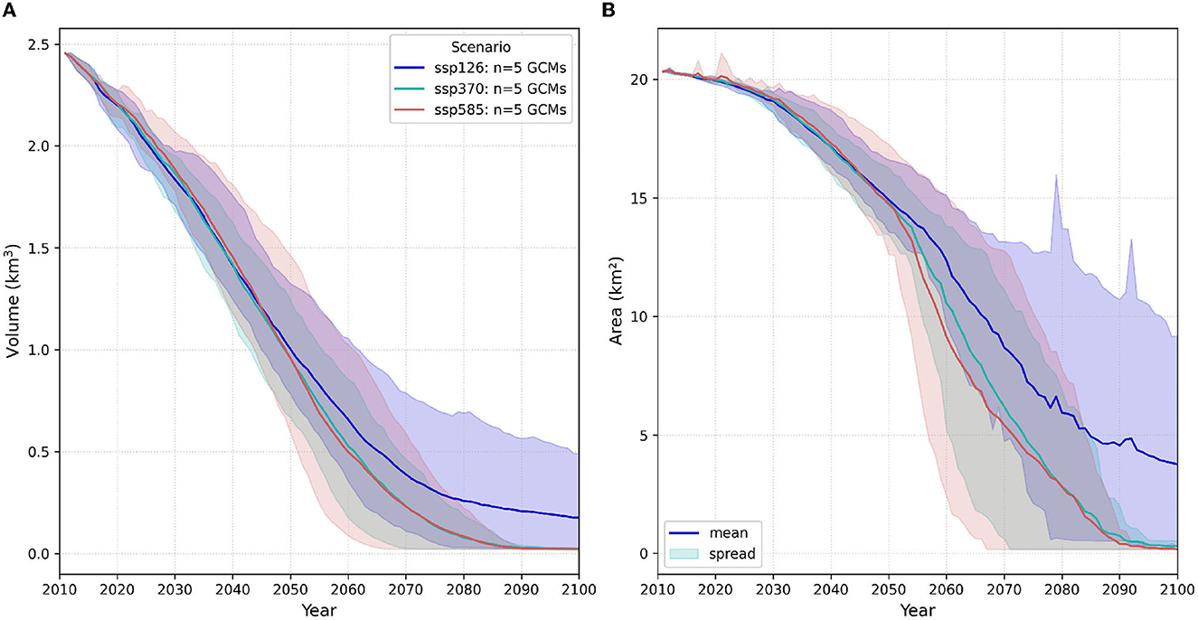
Figure 11. OGGM results with climate data from ISIMIP3b: (A) volume evolution of the glaciers in the study area and (B) area evolution. The values represent the ensemble mean of the five GCMs and for three SSPs: SSP126 (blue), SSP370 (turquoise), and SSP585 (red).

The diagram on the left of Figure 11 shows the evolution of the glaciers' volume, and on the right, the glacierized areas in Gepatschalm. At the beginning of the future simulations, in 2011, a volume of 2.5 km³ is estimated, which corresponds to an area of 20.3 km². Although this area is very close to the value obtained with the VA scaling and the coupling scheme, major differences in terms of volumes are observed. In this case, the initial volume is 60% lower than the VA scaling estimate and 20% higher than the value obtained from the coupling scheme. However, when analyzing certain future years, there seems to be more similarity between the results provided by the ISIMIP3b-OGGM run and the coupling scheme. Table 3 presents the projected volume obtained from each simulation and for three future years: 2040, 2070 and 2100. The values are an ensemble mean of all climate models and refer to RCP2.6/SSP126 and RCP8.5/SSP585.

Table 3

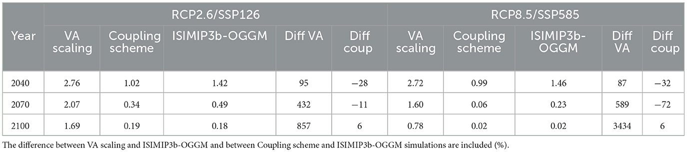
Table 3. Glacier volume predictions for the years 2040, 2070, and 2100 from the different models [VA scaling, coupling scheme, and ISIMIP3b-OGGM (values are in km³)].

Except for RCP8.5 and 2070, the simulated volumes obtained from ISIMIP3b-OGGM and the coupling scheme differ by < 32%. However, the differences are much higher when comparing ISIMIP3b-OGGM with the VA scaling results. The similarities between results from the coupling scheme and OGGM forced by CMIP6 are expected, since both glacier models follow the same ice-flow dynamics. The disparities are likely attributed to the climate models used in each case, which generally represent the main source of uncertainty (Marzeion et al., 2020). The selection of the initial ice volume (in this case in 2011) is crucial for future predictions, since different ice thicknesses could significantly affect glacier evolution as determined by van Tricht et al. (2023). The coupling scheme calculates the initial volume based on the distributed ice thickness using the OGGM depth-integrated flowline model, while the VA scaling approach provides a rough estimate of the initial volume by multiplying the initial area by a mean ice thickness. Furthermore, this mean ice thickness (represented by b in Equation 1) remains constant over time, suggesting that the glaciers will keep the same mean ice thickness until the end of the century. Additionally, the factors involved in Equation (1) are “global” and uniform throughout the catchment and cannot be adjusted on a per glacier basis. This implies that all glaciers are affected by the same thickness, which might well not be the case, especially considering the diversity of glacier sizes within the study area. The coupling scheme is however able to deal with both issues by annually updating the geometries of the glaciers, including the distribution of ice thickness on a per glacier basis.

In any case, and to gain deeper understanding of the VA scaling approach, we also performed a sensitivity analysis on the parameters affecting Equation (1), to see for instance how different mean ice thicknesses (b in Equation 1) influence the results. Our findings demonstrate that, in terms of runoff, neither parameter was sensitive during the historical simulations. Additionally, results from the sensitivity test on the scaling exponent conducted by Radić et al. (2007) indicate that when estimating volume changes over a 100-year period, differences of up to 86% on this factor have negligible effects on results (< 6%). Consequently, the use of fixed (and default) values might be justified, which also align with the values reviewed by Grinsted (2013). Nevertheless, the b factor in Equation (1) exerts a major influence on future projections. As an example, we performed an additional simulation with b = 60 m (the default value is 28.5 m), which represents an average thickness of the glaciers in the catchment (Fischer and Kuhn, 2013). The projected mean annual runoff for RCP4.5 during 2071–2100 increases from 1,419 to 1,527 mm when changing the default value to 60 m. In terms of glacierized areas, the expected glacier coverage increases from 9.4 to 14.6 km², as opporsed to the default set-up (for RCP4.5). This high variability in simulation results under future projections raises concerns about applying the VA scaling approach to estimate runoff in highly glacierized catchments, and places more trust in the use of global glacier models such as OGGM.

3.3 Applicability of the coupling scheme in other catchments

Although the WaSiM-OGGM coupling scheme has only been applied to the Gepatschalm area so far, its use could be extended to any other glacierized catchment. This might be particularly advantageous, for example, in catchments where glacier observations are not available. In this case, the annual glacier outputs generated from OGGM allow to perform model simulations starting at any desired year, hence overcoming dependence on observed outlines. Furthermore, the successful application of both models in water-scarce regions (examples of studies carried out with WaSiM can be found in Cornelissen et al., 2013; Idrissou et al., 2020; Pesci et al., 2023 and with OGGM, in Dixit et al., 2021; Ross et al., 2023) encourages the use of the coupling scheme in such areas. As a changing climate may significantly impact water availability by the end of the century, the prediction of the catchment's hydrological response becomes crucial. Consequently, a deeper understanding of glacier evolution and its contribution to runoff can lead to more effective management of water resources in water-scarce regions.

4 Conclusions

Glacier processes are of major importance to the hydrological response of a catchment, especially when making predictions under future climatic conditions. The WaSiM-OGGM coupling scheme developed in this study has proved to be a step forward in the representation of glaciers and their contribution to runoff generation when looking at different future climate scenarios. The integration of OGGM's detailed ice-flow dynamics representation into the physically-based hydrological WaSiM model enhanced overall runoff performance during the historical period and improved predictions of runoff and glacier evolution in the future. The obtained results align with similar studies, ensuring greater reliability.

The VA scaling approach has shown to be robust during historical simulations, where different values of b lead to similar results. Nevertheless, selecting this parameter has a significant effect on the model's performance for future time periods. Therefore, adopting a singular value for the entire simulation period and catchment as a whole may not be suitable when analyzing different scenarios. This issue is tackled by the WaSiM-OGGM coupling scheme, since an annual update of the glacier volumes and areas is fed into the model, thus no longer being dependent on the VA scaling relation.

The determination of the glacier's geometry from OGGM is based on an approximation, which led to some deficiencies and hence to a slight underestimation of the total glacier area. This issue, combined with the unknown initial conditions of the glaciers in the past, might be the cause of the underestimations in terms of initial areas, compared to the observed values. With the constant advances in modeling and programming, it could be feasible to improve the delineation of the glacier geometries and therefore obtain a more accurate representation. In addition, a more thorough method could be adopted for initializing OGGM, in which glaciers are reconstructed based on climate information and their current geometry (Eis et al., 2021). Furthermore, the coupling scheme could also be adapted to the next generation of mass balance models, in which, for example, a higher temporal resolution could be used (Schuster et al., 2023).

We are confident in the efficacy of the coupling scheme when performing simulations with little or even no glacier observations, since OGGM (and consequently the coupling scheme) can be initialized in any year. Finally, it is worth noting that the WaSiM-OGGM coupling scheme is accessible as open-source software (Pesci, 2023), allowing for the prediction of the hydrological response of any mountainous catchment without necessitating additional expertise in glacier modeling. This is particularly valuable in areas where water scarcity may become a critical issue.

Data availability statement

The datasets presented in this study can be found in online repositories. The names of the repository/repositories and accession number(s) can be found below: https://doi.org/10.5281/ZENODO.8315508; https://github.com/p-s-o/simple-knn-weather-data-disaggregation.

Author contributions

MP: Conceptualization, Software, Visualization, Writing – original draft, Methodology. PS: Software, Writing – review & editing. TB: Data curation, Writing – review & editing. KF: Conceptualization, Funding acquisition, Project administration, Supervision, Validation, Writing – review & editing.

Funding

The author(s) declare financial support was received for the research, authorship, and/or publication of this article. This study was carried out in the framework of the DIRT-X project, which is part of AXIS, an ERA-NET initiated by JPI Climate, and funded by FFG Austria, BMBF Germany (FKZ: 01LS1902B), FORMAS Sweden, NWO NL, and RCN Norway with co-funding from the European Union (Grant No. 776608).

Acknowledgments

We acknowledge the World Climate Research Programme's Working Group on Regional Climate, and the Working Group on Coupled Modeling, former coordinating body of CORDEX and responsible panel for CMIP5. We also thank the climate modeling groups (listed in Table 1 of this paper) for producing and making available their model output. We also acknowledge the Earth System Grid Federation infrastructure an international effort led by the U.S. Department of Energy's Program for Climate Model Diagnosis and Intercomparison, the European Network for Earth System Modelling and other partners in the Global Organisation for Earth System Science. We also acknowledge the provision of the INCA data by the University of Innsbruck and the provision of the runoff data by TIWAG. Another thanks goes to Martin Stocker-Waldhuber for the provision of the mass balance data at Gepatschferner. Finally, we extend our gratitude to Ross Pidoto for proofreading the manuscript, and to the reviewers and Nicole Schaffer for their enriching discussions and enormous help in improving the manuscript. The publication of this article was funded by the Open Access Fund of Leibniz Universität Hannover.

Conflict of interest

The authors declare that the research was conducted in the absence of any commercial or financial relationships that could be construed as a potential conflict of interest.

Publisher's note

All claims expressed in this article are solely those of the authors and do not necessarily represent those of their affiliated organizations, or those of the publisher, the editors and the reviewers. Any product that may be evaluated in this article, or claim that may be made by its manufacturer, is not guaranteed or endorsed by the publisher.

Supplementary material

The Supplementary Material for this article can be found online at: https://www.frontiersin.org/articles/10.3389/frwa.2023.1296344/full#supplementary-material

Footnotes

1. ^It is worth noting that this option does not exist for firn and ice melt. These components can only be represented by the T-index method. In order to warrant consistency between both mass balance computations in WaSiM and in OGGM, all runoff components originating from glaciers are computed using the T-index model in WaSiM likewise.

References

Bahr, D. B., Meier, M. F., and Peckham, S. D. (1997). The physical basis of glacier volume-area scaling. J. Geophys. Res. Atmosp. 102, 20355–20362. doi: 10.1029/97JB01696

Crossref Full Text | Google Scholar

Bahr, D. B., Pfeffer, W. T., and Kaser, G. (2015). A review of volume-area scaling of glaciers. Rev. Geophys. 53, 95–140. doi: 10.1002/2014RG000470

PubMed Abstract | Crossref Full Text | Google Scholar

Berg, P., Bosshard, T., Yang, W., and Zimmermann, K. (2022). MIdASv0.2.1 - MultI-scale bias adjuStment. Geosci. Model Dev. 15, 6165–6180. doi: 10.5194/gmd-15-6165-2022

Crossref Full Text | Google Scholar

Buckel, J., and Otto, J.-C. (2018). The austrian glacier inventory gi 4 (2015) in arcgis (shapefile) format, supplement to: Buckel, johannes; otto, jan-christoph; prasicek, günther; keuschnig, markus (2018): Glacial lakes in austria—distribution and formation since the little ice age. Glob. Planet. Change 164, 39–51. doi: 10.1016/j.gloplacha.2018.03.003

Crossref Full Text | Google Scholar

Chen, J., and Ohmura, A., (eds.). (1990). Estimation of Alpine Glacier Water Resources and Their Changes Since the 1870s, Vol. 193. Lausanne: IAHS.

Google Scholar

Chiarle, M., Paranunzio, R., Nigrelli, G., Mortara, G., Terzago, S., von Hardenberg, J., et al. (2020). Forecasting alpine glacier evolution at the seasonal/multiannual scale. doi: 10.5194/egusphere-egu2020-13289

Crossref Full Text | Google Scholar

Cochand, M., Christe, P., Ornstein, P., and Hunkeler, D. (2019). Groundwater storage in high alpine catchments and its contribution to streamflow. Water Resour. Res. 55, 2613–2630. doi: 10.1029/2018WR022989

Crossref Full Text | Google Scholar

Cornelissen, T., Diekkrüger, B., and Giertz, S. (2013). A comparison of hydrological models for assessing the impact of land use and climate change on discharge in a tropical catchment. J. Hydrol. 498, 221–236. doi: 10.1016/j.jhydrol.2013.06.016

Crossref Full Text | Google Scholar

Dixit, A., Sahany, S., and Kulkarni, A. V. (2021). Glacial changes over the Himalayan Beas basin under global warming. J. Environ. Manage. 295, 113101. doi: 10.1016/j.jenvman.2021.113101

PubMed Abstract | Crossref Full Text | Google Scholar

Duan, Q., Sorooshian, S., and Gupta, V. K. (1994). Optimal use of the sce-ua global optimization method for calibrating watershed models. J. Hydrol. 158, 265–284. doi: 10.1016/0022-1694(94)90057-4

Crossref Full Text | Google Scholar

Duethmann, D., Bolch, T., Farinotti, D., Kriegel, D., Vorogushyn, S., Merz, B., et al. (2015). Attribution of streamflow trends in snow and glacier melt-dominated catchments of the Tarim River, Central Asia. Water Resour. Res. 51, 4727–4750. doi: 10.1002/2014WR016716

Crossref Full Text | Google Scholar

Eis, J., van der Laan, L., Maussion, F., and Marzeion, B. (2021). Reconstruction of past glacier changes with an ice-flow glacier model: proof of concept and validation. Front. Earth Sci. 9, 595755. doi: 10.3389/feart.2021.595755

Crossref Full Text | Google Scholar

Ersi, K., Chaohai, L., Zichu, X., Xin, L., and Yongping, S. (2009). Assessment of glacier water resources based on the glacier inventory of China. Ann. Glaciol. 50, 104–110. doi: 10.3189/172756410790595822

Crossref Full Text | Google Scholar

Eyring, V., Bony, S., Meehl, G. A., Senior, C. A., Stevens, B., Stouffer, R. J., et al. (2016). Overview of the coupled model intercomparison project phase 6 (cmip6) experimental design and organization. Geosci. Model Dev. 9, 1937–1958. doi: 10.5194/gmd-9-1937-2016

Crossref Full Text | Google Scholar

Fischer, A., and Kuhn, M. (2013). Ground-penetrating radar measurements of 64 austrian glaciers between 1995 and 2010. Ann. Glaciol. 54, 179–188. doi: 10.3189/2013AoG64A108

Crossref Full Text | Google Scholar

Fischer, A., Seiser, B., Stocker-Waldhuber, M., Mitterer, C., and Abermann, J. (2015). The austrian glacier inventories gi 1 (1969), gi 2 (1998), gi 3 (2006), and gi lia in arcgis (shapefile) format, supplement to: Fischer, andrea; seiser, bernd; stocker-waldhuber, martin; mitterer, christian; abermann, jakob (2015): Tracing glacier changes in austria from the little ice age to the present using a lidar-based high-resolution glacier inventory in austria. Cryosphere 9, 753–766. doi: 10.5194/tc-9-753-2015

Crossref Full Text | Google Scholar

Förster, K., Garvelmann, J., Meißl, G., and Strasser, U. (2018). Modelling forest snow processes with a new version of wasim. Hydrol. Sci. J. 63, 1540–1557. doi: 10.1080/02626667.2018.1518626

Crossref Full Text | Google Scholar

Freudiger, D., Kohn, I., Seibert, J., Stahl, K., and Weiler, M. (2017). Snow redistribution for the hydrological modeling of alpine catchments: snow redistribution for hydrological modeling. Wiley Interdiscip. Rev. Water 4, e1232. doi: 10.1002/wat2.1232

Crossref Full Text | Google Scholar

Grinsted, A. (2013). An estimate of global glacier volume. Cryosphere 7, 141–151. doi: 10.5194/tc-7-141-2013

Crossref Full Text | Google Scholar

Gupta, H. V., Kling, H., Yilmaz, K. K., and Martinez, G. F. (2009). Decomposition of the mean squared error and nse performance criteria: implications for improving hydrological modelling. J. Hydrol. 377, 80–91. doi: 10.1016/j.jhydrol.2009.08.003

Crossref Full Text | Google Scholar

Gupta, H. V., Sorooshian, S., and Yapo, P. O. (1998). Toward improved calibration of hydrologic models: multiple and noncommensurable measures of information. Water Resour. Res. 34, 751–763. doi: 10.1029/97WR03495

Crossref Full Text | Google Scholar

Haiden, T., Kann, A., Wittmann, C., Pistotnik, G., Bica, B., and Gruber, C. (2011). The integrated nowcasting through comprehensive analysis (inca) system and its validation over the Eastern Alpine region. Weather Forecast. 26, 166–183. doi: 10.1175/2010WAF2222451.1

Crossref Full Text | Google Scholar

Hanzer, F., Förster, K., Nemec, J., and Strasser, U. (2018). Projected cryospheric and hydrological impacts of 21st century climate change in the ötztal alps (Austria) simulated using a physically based approach. Hydrol. Earth Syst. Sci. 22, 1593–1614. doi: 10.5194/hess-22-1593-2018

Crossref Full Text | Google Scholar

Hanzer, F., Helfricht, K., Marke, T., and Strasser, U. (2016). Multilevel spatiotemporal validation of snow/ice mass balance and runoff modeling in glacierized catchments. Cryosphere 10, 1859–1881. doi: 10.5194/tc-10-1859-2016

Crossref Full Text | Google Scholar

Hock, R. (1999). A distributed temperature-index ice- and snowmelt model including potential direct solar radiation. J. Glaciol. 45, 101–111. doi: 10.3189/S0022143000003087

Crossref Full Text | Google Scholar

Houska, T., Kraft, P., Chamorro-Chavez, A., and Breuer, L. (2015). Spotting model parameters using a ready-made python package. PLoS ONE 10, e0145180. doi: 10.1371/journal.pone.0145180

PubMed Abstract | Crossref Full Text | Google Scholar

Hugonnet, R., McNabb, R., Berthier, E., Menounos, B., Nuth, C., Girod, L., et al. (2021). Accelerated global glacier mass loss in the early twenty-first century. Nature 592, 726–731. doi: 10.1038/s41586-021-03436-z

PubMed Abstract | Crossref Full Text | Google Scholar

Huss, M. (2011). Present and future contribution of glacier storage change to runoff from macroscale drainage basins in europe. Water Resour. Res. 47. doi: 10.1029/2010WR010299

Crossref Full Text | Google Scholar

Huss, M., Farinotti, D., Bauder, A., and Funk, M. (2008). Modelling runoff from highly glacierized alpine drainage basins in a changing climate. Hydrol. Process. 22, 3888–3902. doi: 10.1002/hyp.7055

Crossref Full Text | Google Scholar

Huss, M., and Hock, R. (2015). A new model for global glacier change and sea-level rise. Front. Earth Sci. 3, 54. doi: 10.3389/feart.2015.00054

Crossref Full Text | Google Scholar

Huss, M., Jouvet, G., Farinotti, D., and Bauder, A. (2010). Future high-mountain hydrology: a new parameterization of glacier retreat. Hydrol. Earth Syst. Sci. 14, 815–829. doi: 10.5194/hess-14-815-2010

Crossref Full Text | Google Scholar

Idrissou, M., Diekkrüger, B., Tischbein, B., Ibrahim, B., Yira, Y., Steup, G., et al. (2020). Testing the robustness of a physically-based hydrological model in two data limited inland valley catchments in Dano, Burkina Faso. Hydrology 7, 43. doi: 10.3390/hydrology7030043

Crossref Full Text | Google Scholar

Jacob, D., Petersen, J., Eggert, B., Alias, A., Christensen, O. B., Bouwer, L. M., et al. (2013). Euro-cordex: new high-resolution climate change projections for European impact research. Reg. Environ. Change 14, 563–578. doi: 10.1007/s10113-013-0499-2

Crossref Full Text | Google Scholar

Khadka, M., Kayastha, R. B., and Kayastha, R. (2020). Future projection of cryospheric and hydrologic regimes in Koshi River basin, Central Himalaya, using coupled glacier dynamics and glacio-hydrological models. J. Glaciol. 66, 831–845. doi: 10.1017/jog.2020.51

Crossref Full Text | Google Scholar

Koboltschnig, G. R., and Schöner, W. (2011). The relevance of glacier melt in the water cycle of the alps: the example of Austria. Hydrol. Earth Syst. Sci. 15, 2039–2048. doi: 10.5194/hess-15-2039-2011

Crossref Full Text | Google Scholar

Kormann, C., Bronstert, A., Francke, T., Recknagel, T., and Graeff, T. (2016). Model-based attribution of high-resolution streamflow trends in two alpine basins of Western Austria. Hydrology 3, 7. doi: 10.3390/hydrology3010007

Crossref Full Text | Google Scholar

Lall, U., and Sharma, A. (1996). A nearest neighbor bootstrap for resampling hydrologic time series. Water Resour. Res. 32, 679–693. doi: 10.1029/95WR02966

Crossref Full Text | Google Scholar

Lange, S. (2019). Wfde5 Over Land Merged With era5 Over the Ocean (w5e5) Potsdam: GFZ Data Services. doi: 10.5880/pik.2019.023

Crossref Full Text | Google Scholar

Lange, S., Quesada-Chacón, D., and Büchner, M. (2023). Secondary ISIMIP3b bias-adjusted atmospheric climate input data (v1.2). Potsdam: ISIMIP. doi: 10.48364/ISIMIP.581124.2

Crossref Full Text | Google Scholar

Marzeion, B., Hock, R., Anderson, B., Bliss, A., Champollion, N., Fujita, K., et al. (2020). Partitioning the uncertainty of ensemble projections of global glacier mass change. Earths Fut. 8. doi: 10.1029/2019EF001470

Crossref Full Text | Google Scholar

Marzeion, B., Jarosch, A. H., and Hofer, M. (2012). Past and future sea-level change from the surface mass balance of glaciers. Cryosphere 6, 1295–1322. doi: 10.5194/tc-6-1295-2012

Crossref Full Text | Google Scholar

Maussion, F., Butenko, A., Champollion, N., Dusch, M., Eis, J., Fourteau, K., et al. (2019). The open global glacier model (oggm) v1.1. Geosci. Model Dev. 12, 909–931. doi: 10.5194/gmd-12-909-2019

Crossref Full Text | Google Scholar

Maussion, F., Rothenpieler, T., Dusch, M., Schmitt, P., Vlug, A., Schuster, L., et al. (2023). Oggm/oggm: v1.6.0. Zenodo. doi: 10.5281/zenodo.7718476

Crossref Full Text | Google Scholar

Meier, M. F. (1969). Glaciers and water supply. J. Am. Water Works Assoc. 61, 8–12. doi: 10.1002/j.1551-8833.1969.tb03696.x

Crossref Full Text | Google Scholar

Moriasi, D. N., Arnold, J. G., van Liew, M. W., Bingner, R. L., Harmel, R. D., and Veith, T. L. (2007). Model evaluation guidelines for systematic quantification of accuracy in watershed simulations. Transact. ASABE 50, 885–900. doi: 10.13031/2013.23153

Crossref Full Text | Google Scholar

Naz, B. S., Frans, C. D., Clarke, G. K. C., Burns, P., and Lettenmaier, D. P. (2014). Modeling the effect of glacier recession on streamflow response using a coupled glacio-hydrological model. Hydrol. Earth Syst. Sci. 18, 787–802. doi: 10.5194/hess-18-787-2014

Crossref Full Text | Google Scholar

Patzelt, G. (2013). Austrian Glacier Inventory 1969 (g i). Bremen: Pangaea.

Google Scholar

Pesci, M. H. (2023). Wasim-oggm: v1.0.1. Zenodo. doi: 10.5281/zenodo.8315508

Crossref Full Text | Google Scholar

Pesci, M. H., Mouris, K., Haun, S., and Förster, K. (2023). Assessment of uncertainties in a complex modeling chain for predicting reservoir sedimentation under changing climate. Model. Earth Syst. Environ. 9, 3777–3793. doi: 10.1007/s40808-023-01705-6

Crossref Full Text | Google Scholar

Radić, V., and Hock, R. (2014). Glaciers in the earth's hydrological cycle: assessments of glacier mass and runoff changes on global and regional scales. Surv. Geophys. 35, 813–837. doi: 10.1007/s10712-013-9262-y

Crossref Full Text | Google Scholar

Radić, V., Hock, R., and Oerlemans, J. (2007). Volume-area scaling vs flowline modelling in glacier volume projections. Ann. Glaciol. 46, 234–240. doi: 10.3189/172756407782871288

Crossref Full Text | Google Scholar

RGI Consortium (2017). Randolph Glacier Inventory 6.0. National Snow and Ice Data Center. doi: 10.7265/4M1F-GD79

Crossref Full Text | Google Scholar

Ross, A. C., Mendoza, M. M., Drenkhan, F., Montoya, N., Baiker, J. R., Mackay, J. D., et al. (2023). Seasonal water storage and release dynamics of Bofedal wetlands in the Central Andes. Hydrol. Process. 37. doi: 10.1002/hyp.14940

Crossref Full Text | Google Scholar

Rounce, D. R., Hock, R., and Shean, D. E. (2020). Glacier mass change in high mountain Asia through 2100 using the open-source python glacier evolution model (pygem). Front. Earth Sci. 7, 331. doi: 10.3389/feart.2019.00331

Crossref Full Text | Google Scholar

Schaefli, B., and Gupta, H. V. (2007). Do nash values have value? Hydrol. Process. 21, 2075–2080. doi: 10.1002/hyp.6825

Crossref Full Text | Google Scholar

Schaffer, N., MacDonell, S., Réveillet, M., Yáñez, E., and Valois, R. (2019). Rock glaciers as a water resource in a changing climate in the semiarid chilean Andes. Reg. Environ. Change 19, 1263–1279. doi: 10.1007/s10113-018-01459-3

Crossref Full Text | Google Scholar

Schöber, J., Achleitner, S., Kirnbauer, R., Schöberl, F., and Schönlaub, H. (2010). Hydrological modelling of glacierized catchments focussing on the validation of simulated snow patterns-applications within the flood forecasting system of the Tyrolean River Inn. Adv. Geosci. 27, 99–109. doi: 10.5194/adgeo-27-99-2010

Crossref Full Text | Google Scholar

Schulla, J. (1997). Hydrologische Modellierung von Flussgebieten zur Absch#tzung der Folgen von Klimaänderungen (Dissertation), ETH, Zurich, Switzerland.

Google Scholar

Schulla, J. (2021). Model Description Wasim. Zürich: Hydrology Software Consulting.

Google Scholar

Schuster, L., Rounce, D. R., and Maussion, F. (2023). Glacier projections sensitivity to temperature-index model choices and calibration strategies. Ann. Glaciol. 1–16. doi: 10.1017/aog.2023.57

Crossref Full Text | Google Scholar

Stahl, K., Moore, R. D., Shea, J. M., Hutchinson, D., and Cannon, A. J. (2008). Coupled modelling of glacier and streamflow response to future climate scenarios. Water Resour. Res. 44. doi: 10.1029/2007WR005956

Crossref Full Text | Google Scholar

Stocker-Waldhuber, M. (2019). Multi-Method Investigation of Dynamic Processes in Rapidly Changing Alpine Glaciers (Dissertation), Katolische Universität Eichstätt-Inglostadt, Eichstätt-Inglostadt.

Google Scholar

Stoll, E., Hanzer, F., Oesterle, F., Nemec, J., Schöber, J., Huttenlau, M., et al. (2020). What can we learn from comparing glacio-hydrological models? Atmosphere 11, 981. doi: 10.3390/atmos11090981

Crossref Full Text | Google Scholar

Strasser, U., Bernhardt, M., Weber, M., Liston, G. E., and Mauser, W. (2008). Is snow sublimation important in the alpine water balance? Cryosphere 2, 53–66. doi: 10.5194/tc-2-53-2008

Crossref Full Text | Google Scholar

Tarasova, L., Knoche, M., Dietrich, J., and Merz, R. (2016). Effects of input discretization, model complexity, and calibration strategy on model performance in a data-scarce glacierized catchment in Central Asia. Water Resour. Res. 52, 4674–4699. doi: 10.1002/2015WR018551

Crossref Full Text | Google Scholar

Thornton, J. M., Brauchli, T., Mariethoz, G., and Brunner, P. (2021). Efficient multi-objective calibration and uncertainty analysis of distributed snow simulations in rugged alpine terrain. J. Hydrol. 598, 126241. doi: 10.1016/j.jhydrol.2021.126241

Crossref Full Text | Google Scholar

van Tiel, M., Stahl, K., Freudiger, D., and Seibert, J. (2020). Glacio-hydrological model calibration and evaluation. WIREs Water 66, 249. doi: 10.1002/wat2.1483

Crossref Full Text | Google Scholar

van Tricht, L., Zekollari, H., Huss, M., Farinotti, D., and Huybrechts, P. (2023). Global vs local glacier modelling: a comparison in the Tien Shan. doi: 10.5194/tc-2023-87

Crossref Full Text | Google Scholar

Verbunt, M., Gurtz, J., Jasper, K., Lang, H., Warmerdam, P., and Zappa, M. (2003). The hydrological role of snow and glaciers in alpine river basins and their distributed modeling. J. Hydrol. 282, 36–55. doi: 10.1016/S0022-1694(03)00251-8

Crossref Full Text | Google Scholar

Wiersma, P., Aerts, J., Zekollari, H., Hrachowitz, M., Drost, N., Huss, M., et al. (2022). Coupling a global glacier model to a global hydrological model prevents underestimation of glacier runoff. Hydrol. Earth Syst. Sci. 26, 5971–5986. doi: 10.5194/hess-26-5971-2022

Crossref Full Text | Google Scholar

Winter, B., Schneeberger, K., Dung, N. V., Huttenlau, M., Achleitner, S., Stötter, J., et al. (2019). A continuous modelling approach for design flood estimation on sub-daily time scale. Hydrol. Sci. J. 64, 539–554. doi: 10.1080/02626667.2019.1593419

Crossref Full Text | Google Scholar

Wood, L. R., Neumann, K., Nicholson, K. N., Bird, B. W., Dowling, C. B., and Sharma, S. (2020). Melting himalayan glaciers threaten domestic water resources in the mount everest region, Nepal. Front. Earth Sci. 8, 128. doi: 10.3389/feart.2020.00128

Crossref Full Text | Google Scholar

Zekollari, H., Huss, M., and Farinotti, D. (2019). Modelling the future evolution of glaciers in the european alps under the euro-cordex rcm ensemble. Cryosphere 13, 1125–1146. doi: 10.5194/tc-13-1125-2019

Crossref Full Text | Google Scholar

Zemp, M., Huss, M., Thibert, E., Eckert, N., McNabb, R., Huber, J., et al. (2019). Global glacier mass changes and their contributions to sea-level rise from 1961 to 2016. Nature 568, 382–386. doi: 10.1038/s41586-019-1071-0

PubMed Abstract | Crossref Full Text | Google Scholar