
95% of researchers rate our articles as excellent or good
Learn more about the work of our research integrity team to safeguard the quality of each article we publish.
Find out more
ORIGINAL RESEARCH article
Front. Water , 21 December 2023
Sec. Water and Built Environment
Volume 5 - 2023 | https://doi.org/10.3389/frwa.2023.1287357
 Mohamed Galal Eltarabily1,2
 Hany Farhat Abd-Elhamid3,4
 Martina Zeleňáková5*
 Mohamed Kamel Elshaarawy6Mohamed Elkiki1,7
 Tarek Selim1
Introduction: Efficient water resource management in irrigation systems relies on the accurate estimation of seepage loss from lined canals. This study utilized machine learning (ML) algorithms to tackle this challenge in seepage loss prediction.
Methods: Firstly, seepage flow through irrigation canals was modeled numerically and experimentally using Slide2 and physical models, respectively. Then, the Slide2 model results were compared to the experimental tests. Thus, the model was used to conduct 600 simulation scenarios. A parametric analysis was performed to investigate the effect of canal geometry and liner properties on seepage loss. Based on the conducted scenarios, ML models were developed and evaluated to determine the best predictive model. The ML models included non-ensemble (regression-based, evolutionary, neural network) and ensemble models. Non-ensemble models (adaptive boosting, random forest, gradient boosting). There were four input ratios in these models: bed width to water depth, side slope, liner to soil hydraulic conductivity, and liner thickness to water depth. The output variable was the seepage loss ratio. Seven performance indices and k-fold cross-validation were employed to evaluate reliability and accuracy. Moreover, a sensitivity analysis was conducted to investigate the significance of each input in predicting seepage loss.
Results and discussion: The findings revealed that the Artificial Neural Network (ANN) model was the most dependable predictor, achieving the highest determination-coefficient (R2) value of 0.997 and root-mean-square-error (RMSE) of 0.201. The eXtreme Gradient Boosting (XGBoost) followed the ANN model closely, which achieved an R2 of 0.996 and RMSE of 0.246. Sensitivity analysis showed that liner hydraulic conductivity is the most significant parameter, contributing 62% predictive importance, while the side slope has the lowest significance. In conclusion, this study presented efficient and cost-effective models for predicting seepage loss, eliminating the need for resource-intensive experimental or field investigations.
Water scarcity is increasing due to climate change. This increase underscores the necessity to investigate water losses. It is essential to improve water management, especially in water-scarce regions. Irrigation is regarded as one of the most essential water uses. Water is lost in irrigation canals due to seepage and evaporation, but evaporation losses are insignificant in comparison (Waller and Yitayew, 2015). Seepage occurs when water percolates into the soil through the wetted perimeter of the canal (Jamel, 2016). Seepage can be severe if the soil through which the canal passes is porous and the canal is unlined. Thus, preventing or controlling canal seepage loss improves water resource utilization efficiency (Swamee et al., 2000).
Measuring canal seepage loss involves various methods, such as field measurements, analytical formulas, empirical equations, and numerical modeling (Vishnoi and Saxena, 2014; Christian and Trivedi, 2018). Field measurements include the ponding method, the inflow–outflow method, and point measurements (Waller and Yitayew, 2015), but their implementation can be difficult due to practical constraints (Eltarabily and Negm, 2015). In contrast, numerical models offer flexibility and speed and require fewer inputs, making them increasingly popular for estimating canal seepage loss (Elkamhawy et al., 2021).
To effectively estimate seepage loss using numerical models, selecting consistent boundary conditions and developing seepage models based on these conditions is crucial. Previous research has explored seepage from earthen canals through direct measurements (Lund et al., 2023) or analytical studies (Sharma and Chawla, 1979; Chahar, 2007; Osman and Rahman, 2008; Ghazaw, 2011; Carabineanu, 2012; Uchdadiya and Patel, 2014). Empirical equations have been used and compared in earlier studies (Mowafy, 2001; Saha, 2015), while more recent research increasingly uses numerical modeling techniques (Salmasi and Abraham, 2020; El-Molla and El-Molla, 2021a,b; El-Molla and Eltarabily, 2023; Eltarabily et al., 2023a,b).
Lining irrigation canals is considered one of the most efficient ways to reduce water losses in water-conveying systems (Abd-Elaty et al., 2022). Canal lining improves flow characteristics, reduces seepage loss, controls weeds growing, and minimizes maintenance costs. Moreover, it mitigates water logging risks in adjacent low agricultural lands (Abd-elziz et al., 2022). Different lining materials reduce seepage loss, including compacted earth, concrete, flexible membranes, asphaltic concrete, and soil cement mixtures (Waller and Yitayew, 2015).
Studies have explored the impact of different lining materials on seepage loss. Kahlown and Kemper (2005) evaluated the reduction of water losses from watercourses of several types of lining (rectangular brick masonry and concrete trapezoidal sections for canal bed and sides). Results showed a minor difference in losses between earthen and long-term lined watercourses. Bahramlu (2011) investigated seepage loss in irrigated channels with rock cement and concrete lining in cold regions, specifically in Hamedan province, Iran. The results revealed no substantial disparity in the average seepage loss between the concrete-lined channels and those covered with rock cement. Aghvami et al. (2013) employed the SEEP/W model and Evolutionary Polynomial Regression (EPR) modeling techniques to investigate seepage in the Qazvin and Isfahan channels in Iran. Results showed that EPR was more accurate in estimating channel seepage than the SEEP/W model. Jamel (2016) studied the seepage loss from unlined and lined triangular channels using the SEEP/W model. Results showed that the seepage loss increased with higher soil and lining hydraulic conductivities, freeboard, inner side slopes, and channel height (the water depth plus the freeboard).
Salmasi and Abraham (2020) used the SEEP/W model to study the factors affecting seepage from trapezoidal, rectangular, and triangular earth canals and develop linear and non-linear multivariate relationships. Results showed that the wetted perimeter was distinguished as an effective parameter in the seepage from the canals, while the canal's inner side slope had a low impact on the seepage. Sharief and Zakwan (2021) compared the performance of a low-density polyethylene (LDPE) lined canal with a random rubble (RR) masonry-lined canal. Results showed that the seepage loss from LDPE lining was calculated as 2% compared to 8% from RR lining. Hosseinzadeh Asl et al. (2020) investigated the impact of hydraulic and geometric parameters on seepage loss in an unlined channel by the SEEP/W model and the empirical relationships. Results showed that the SEEP/W model accurately estimated seepage loss compared to the empirical relationships. Moreover, the empirical relationships had excessive errors. El-Molla and El-Molla (2021a) used the SEEP/W model to explore the impact of compacted earth lining on the amount of seepage discharges. Results showed that 99.8% of the seepage discharges can be saved if the soil is highly compacted.
Eltarabily et al. (2023a) utilized the FLOW-3D and Slide2 models to estimate the discharge and seepage loss from the canal reaches, respectively. Moreover, the effect of lining on the discharge and seepage loss of the El-Sont Canal in Egypt was investigated using Cement Concrete (CC) and CC with Low-Density Polyethylene (LDPE) film. Results showed that by lining the canal by CC with LDPE film, the discharges of the canal reaches were averagely increased by 150%, while the seepage loss was reduced by 97%. Eltarabily et al. (2023b) used the Slide2 model to investigate the effect of lining on seepage loss from lined irrigation canals. The study considered different groundwater table (GWT) locations, canal berm widths, and liner properties (hydraulic conductivity and liner thickness). The results showed that the liner hydraulic conductivity had the highest effect on seepage loss, irrespective of the GWT location and the canal berm width.
In recent years, machine learning and soft computing techniques have proven robust and reliable in modeling hydraulic and hydrologic processes (Nourani et al., 2012; Elshaarawy and Hamed, 2023). These techniques can handle large, complex, and noisy datasets, making them suitable for simulating seepage when the physical relationships are not fully understood. Balkhair (2002) conducted an ANN to approximate an aquifer's transmissivity and storage coefficient, yielding highly accurate results. Lallahem et al. (2005) conducted an ANN model that effectively simulated groundwater levels within an unconfined sedimentary aquifer in France, highlighting the advantages of utilizing ANN for groundwater level modeling. Samani et al. (2007) developed an ANN for estimating parameters in a non-leaky confined aquifer, providing a simpler and more accurate surrogate than traditional methods. Najafzadeh and Barani (2011) conducted a comprehensive study on predicting scour depth around bridge piers using two methods: Group Method of Data Handling (GMDH) networks developed with Genetic Programming (GP) and Back Propagation (BP) algorithms. The study revealed that while the GMDH-GP model is more time-consuming and complex, it yields more accurate predictions than the GMDH-BP model.
Taormina et al. (2012) developed an ANN for predicting groundwater levels in an unconfined coastal aquifer in Italy. They examined the relationship between groundwater fluctuations and factors such as marine tide, rainfall recharge, and evapotranspiration. The study demonstrated the efficacy of ANN in simulating shallow aquifer groundwater levels. Mohanty et al. (2013) conducted an assessment comparing the predictive capabilities of MODFLOW (a finite difference method) and the ANN model for groundwater flow prediction in an alluvial aquifer. The findings showed that the ANN model outperformed the MODFLOW in predictive accuracy and efficiency. Fallah-Mehdipour et al. (2013) demonstrated the effectiveness of GEP in deriving the governing groundwater flow equations for two aquifers in Iran, highlighting its superior performance. Najafzadeh and Tafarojnoruz (2016) employed neuro-fuzzy-based group method of data handling (NF-GMDH) improved with particle swarm optimization (PSO) to estimate the longitudinal dispersion coefficient in rivers. The results revealed that NF-GMDH-PSO had the highest efficiency for predicting longitudinal dispersion coefficients.
Najafzadeh et al. (2018) explored the impact of debris on scour depth around bridge piers using NF-GMDH models enhanced with various evolutionary algorithms. The results highlighted the significance of the blockage ratio in scour depth prediction, with NF-GMDH-PSO providing the most accurate results among the tested models. Najafzadeh and Saberi-Movahed (2019) utilized the group method of data handling (GMDH), incorporating gene-expression programming (GEP), to predict three-dimensional free-span expansion rates around pipelines affected by waves. The GMDH-GEP model performed well against other models, emphasizing the role of sediment size, pipeline geometry, and wave characteristics in scour rate predictions. Gad et al. (2023) utilized ANN and GEP models to analyze and predict seepage loss. They created new relations using variables such as Manning's coefficient, the Froude number, and the hydraulic radius. The GEP method showed more promising results than ANN in forecasting seepage loss for lined and unlined canal conditions. They reported high determination coefficients, correlation factors, and low RMSE values, signifying the models' robustness for predicting seepage loss.
Based on the above, limited research has addressed seepage loss from lined irrigation canals. Accurate prediction of seepage loss is critical for increasing water efficiency, especially in water-scarce regions. ML models provide a viable alternative by learning complex data-driven relationships between influential factors like canal geometry and liner properties to predict seepage loss. Hence, this study was conducted to predict seepage loss from lined irrigation canals using both ML models (non-ensemble and ensemble). The non-ensemble models were Multiple Linear Regression (MLR), Multiple Non-linear Regression (MNLR), Support Vector Regression (SVR), Gene Expression Programming (GEP), and Artificial Neural Network (ANN). The ensemble models were Adaptive Boosting (AdaBoost), Random Forest (RF), and eXtreme Gradient Boosting (XGBoost).
Furthermore, the performance of the models was assessed using seven performance indices to gauge the accuracy and dependability of the models. Finally, a sensitivity analysis was employed to examine the relationship between input variables in estimating seepage loss from lined irrigation canals. This study can enable water resources specialists and designers to evaluate the effect of the investigated parameters on predicting seepage loss quickly and more economically than costly experimental studies.
Figure 1 shows the research methodology used in this study. Firstly, experimental tests were implemented in a physical model for unlined and lined canals with different configurations. The Slide2 numerical model was then used to estimate the seepage loss, and its results were compared with the physical one. Moreover, the Slide2 model was used to perform multiple scenarios considering different canal geometries and liner properties for estimating seepage loss from lined canals. Based on these scenarios, ML models were developed. Finally, the adopted ML models were evaluated to determine the best predictive model of seepage loss from lined canals.
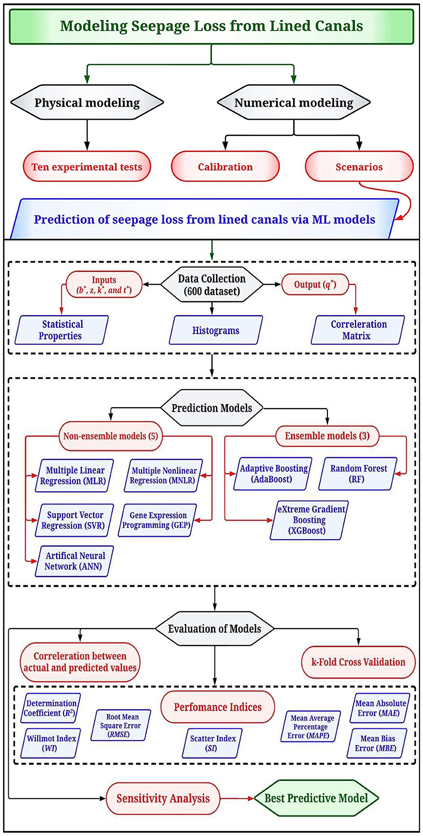
Figure 1. Flowchart of the methodological approach adopted in this study.
The prediction methodology included: (1) dataset was gathered from the Slide2 model scenarios. This data was then assessed for statistical properties using a heatmap and histograms; (2) both non-ensemble and ensemble ML methods were utilized. Results from these models were measured against select performance indices; (3) the data was split into training and test subsets, followed by k-fold cross-validation; and (4) finally, the model's accuracy was determined using specific performance indicators, and a sensitivity analysis was conducted.
This research examined various geometric and hydraulic factors influencing seepage loss from lined irrigation canals (Eltarabily et al., 2023b). The parameters studied included seepage loss per unit length of the canal (q), soil's hydraulic conductivity (k), width of the canal bed (b), depth of water in the canal (y), slope of the canal sides (z), thickness of the liner (tL), and the hydraulic conductivity of the liner (kL). Equation 1 was derived using dimensional analysis, as presented below:
The executed functional relation by applying Buckingham's π theorem (Evans, 1972) was shown in Equation 2 as follows:
The π terms can be expressed in Equation 3 as follows:
Where q* is the seepage losses ratio (q/k. y), b* is the canal geometry ratio (b/y), k* is the liner hydraulic conductivity ratio (kL/k), and t* is the liner thickness ratio (tL/y).
A physical model was constructed in the Irrigation and Hydraulic Laboratory at the Faculty of Engineering, Horus University in Egypt, New Damietta, Egypt. The model was installed inside rectangular tanks made of securit glass of thickness of 1 cm with a length of 100 cm, a width of 50 cm, and a height of 100 cm. The tank bottom was drilled into eight slots of ½ inch diameter and attached with a drainage configuration consisting of a pipe system containing two pipelines ¾ inch diameter with four slots per line. Figure 2 depicts the longitudinal and transverse directions of the physical model and illustrates the inner tank dimensions and the pipe system. The tests were conducted for a half cross-section of unlined and lined symmetrical canals, as shown in Supplementary Figures 1A, B, respectively.
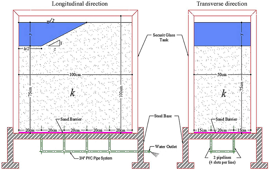
Figure 2. Schematic representation of the implemented physical model in longitudinal and transverse directions.
Firstly, a sand barrier was placed at the tank bottom. Then, the soil was placed and compacted in layers of 20 cm. The canal side slope was compacted to fit the slope 2H:1V. The soil hydraulic conductivity was 0.00825 cm s−1, as determined by laboratory tests. Firstly, the canal section shape was created in the physical model with varying b* ratio. The canal was filled with water to the desired level and maintained at that level to achieve soil saturation with a constant seepage rate. Then, the water was allowed to pass through the channel bed and side slopes by opening the valve at the water outlet of the pipe system. Considering a constant time interval, the water level is lowered, and the final depth is obtained. The seepage losses (Q) were then calculated in cm3 s−1 (Equation 4) using the volumetric method given by Moghazi and Ismail (1997) as follows:
Where W is the average top canal width (cm), L is the canal length (cm), y1 is the initial water depth (cm), y2 is the water depth after time T (cm), P is the average wetted perimeter (cm), t is the time interval between y1 and y2 (s).
For lining experiments, the canal was lined by a cement mixture of thickness 2 cm covering the canal bed and inner side slope. The cement mixture consists of sand, cement, and water in a 2:1:½ ratio (Alrefaei et al., 2023). The sorptivity test was conducted to determine the hydraulic conductivity of the cement mixture (Alsaadawi et al., 2022). The sorptivity test evaluates the water absorption rate by monitoring the increase in sample mass vs. time when only one surface is exposed to water entry via capillary suction. The liner hydraulic conductivity kL was determined from laboratory tests as 1.04 × 10⁻⁶ cm s−1 (ASTM C185-13, 2013).
The Slide2 model was used to estimate the seepage losses from unlined and lined canals (Eltarabily et al., 2023b). It can simulate seepage flow through a porous medium using a built-in finite element groundwater seepage analysis (Rocscience, 2002). The Laplace equation (Equation 5) is the governing equation in the Slide2 model describing steady-state seepage through an isotropic, homogenous porous medium with a constant hydraulic conductivity in two directions (x and y). The equation was given by Harr (1991) as follows:
where H is defined as the potential head.
The Slide2 model was calibrated by conducting ten experimental tests, i.e., five for unlined and five for lined canals, by varying the canal geometry ratio (i.e., b* = 1, 2, 3, 4, and 5). Due to symmetry, only half of the domain was modeled (Supplementary Figure 2). Mesh refinement was used during discretizing the simulation domain to capture any slight change in fluxes within the simulation domain (Rocscience, 2002). The simulation domain was built by 3,000 mesh elements of 3-noded triangles elements type. However, this element size yielded accurate results with less analysis time.
The hydraulic conductivities (k and kL) were obtained from the laboratory tests and defined in the model. The liner thickness (tL) was taken as 2 cm. According to Eltarabily et al. (2023a,b), boundary conditions in the model were set as follows: The perimeter of the canal was assigned a “Total Head” condition. In contrast, the right edge of the domain was set as an impervious “No flow” boundary. At the bottom edge, a “Nodal flow rate” boundary represented the seepage exit face. These boundary conditions are visualized in Supplementary Figure 2. A discharge section was defined at the desired location within the model to estimate seepage loss. With these boundary settings, the seepage analysis was carried out, and the seepage loss was obtained from the discharge section output.
After the calibration process, 600 simulation scenarios were performed using the Slide2 model. The scenarios included five canal geometry ratios (b* = 1, 2, 3, 4, and 5), three values for the inner side slope (z = 1, 1.5, and 2), eight ratios for the liner hydraulic conductivity to soil (k*= 0.0005, 0.001, 0.005, 0.01, 0.05, 0.1, 0.3, and 0.5), and five ratios for the liner thickness to water depth (t*= 0.01, 0.05, 0.1, 0.15, and 0.2). The boundary conditions were defined similarly to the model calibration process. These scenarios were conducted to (1) explore the combined effect of lining and can geometry on the seepage loss; (2) develop both non-ensemble and ensemble ML models to estimate the seepage loss from lined canals; and (3) determine the best accurate model in predicting seepage loss.
The prediction models were formulated using the conducted 600 scenarios. The b*, z, k*, and t* ratios were designated as the inputs to the models, while the q* ratio was designated as the output. Table 1 provides a detailed statistical overview of the dataset, highlighting the minimum and maximum values, standard deviation (SD), and mean values for input and output variables. For best predictive modeling, developing within these parameter ranges is essential. This analysis underscores the extensive range of parameters captured by the dataset, with the SD indicating how the data is distributed around the mean. As the SD values rise, the distribution becomes more enhanced. Supplementary Figure 3 displays a histogram of various input variables. This histogram reveals that the dataset's seepage loss ratio (q*) varies between 0.01 and 12.67. These values indicate that the models can predict the q* ratio within this range. The wide range of variables in the database proved the dataset's credibility. Thus, based on this dataset, the proposed models are prepared to offer accurate predictions for the q* ratio.
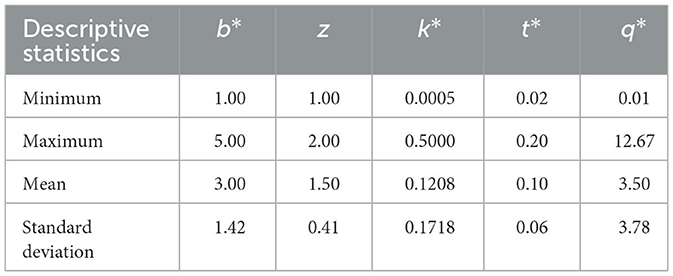
Table 1. Descriptive statistics of the inputs and output.
Variables unrelated to the seepage loss ratio (q*) should be excluded from the dataset, a determination made through correlation analysis. Correlation analysis, by definition, evaluates the relationship between two or more variables. Pearson's correlation coefficient (rxy) is the most recommended and common index (Williams et al., 2020). It is calculated as the ratio of the covariance (cov) of two variables (x, y) to the product of their standard deviations, as represented in Equation (6).
Where and are the mean of two variables (x, y). The ranges of (rxy) are between [−1, 1]. High absolute values of r suggest a strong relationship between the variables and their influence on the outcome. A coefficient of rxy = −1 signifies an inverse linear correlation between the variables. However, a rxy = 0 does not necessarily imply a lack of correlation. When the value of rxy is zero, it does not necessarily imply a lack of correlation because the Pearson correlation coefficient specifically denotes linear relationships.
According to the heatmap of the relationship between two variables (Supplementary Figure 4), k* had the highest effect on q*, as evidenced by its high Pearson correlation coefficient value (r = 0.8). In contrast, the q* ratio is least affected by z, with a correlation of r = 0.07. The figure also shows that the b*, z, and k* ratios positively correlate with the q* ratio. However, the t* ratio was inverse to q* (r = −0.2), suggesting seepage loss decreases with increasing liner thickness. Notably, no uncorrelated parameters indicate that all four input factors can be used to predict seepage loss in lined irrigation canals.
When the scale of input data is inconsistent, some machine learning algorithms may not work efficiently. As illustrated in Table 1, the range of the k* ratio varied between 0.0005 and 0.5, while the t* ratio varied from 0.02 to 0.2. This range suggests significant variation in input values. Data normalization, often rescaling, aligns all input features to a consistent scale. This process accelerates computation and enhances the model's accuracy and robustness. The method primarily employs the max-min mapping technique and can be expressed as in Equation 7:
Where Xn represents the normalized data, while Xmin and Xmax denote the smallest and largest values of every input feature, respectively, and X stands for the original data set undergoing the rescaling process.
This study employed five non-ensemble ML models: MLR, MNLR, SVR, GEP, and ANN. These models were developed using the Statistical Package for the Social Sciences (SPSS) and Matrix Laboratory (MATLAB). The description of each model is illustrated in the following subsections.
Regression models estimate the degree of correlation. These models also determine the relationships between input and output variables. Most Multiple Linear Regression (MLR) models are fitted using the least squares methods. MLR assesses the correlation between a dependent variable and various independent variables, yielding a linear relationship (Neter et al., 1996; Elshaarawy et al., 2023). The formulation for MLR is depicted in Equation 8.
Where Y is the output of a model, a0, a1, a2, …, and am are partial regression coefficients, and Xj's are the input variables.
Non-linear models are simple, interpretable, and predictive (Verma, 2012; Archontoulis and Miguez, 2015). These models can accommodate a wide variety of mean functions. However, they can be less flexible than linear models regarding the data they can describe. However, non-linear models appropriate for a given application can have fewer parameters and are more interpretable. Interpretability comes from associating parameters with a biologically meaningful process.
MNLR model is applied in the following steps: (1) defining the dependent variable, (2) proposing a non-linear equation in which the dependent variable is a function of the independent variables, (3) entering the estimation parameters of the proposed non-linear equation by assuming the starting value; Levenberg-Marquardt was the used estimation method, (4) Finally, the MNLR analysis was started, and the model results were shown in the output log. The expression of MNLR is shown in Equation 9 as follows:
Where Y is the output of a model, a0, a1, a2, …, and am are partial estimation parameters, and Xj's are the input variables.
The Support Vector Machine (SVM) model is commonly utilized in data mining. It is called Support Vector Regression (SVR) when applied to regression problems. SVR has become a widely used tool for classification, prediction, and regression (Cortes and Vapnik, 1995). As a supervised learning method, SVR is particularly suited for tasks involving non-linear regression, limited data sets, and high-dimensional input spaces. The method converts the input data into a higher-dimensional space via a non-linear transformation.
The GEP model was introduced for developing computer programs (Ferreira, 2001). GEP resembled genetic algorithms and genetic programming. GEP output was typically presented as mathematical equations, decision trees, polynomial structures, neural networks, or logical expressions (Ferreira, 2006). Random population chromosomes started the procedure. Expression of the chromosomes determined each individual's fitness. Individuals were selected for their ability to reproduce after genetic modification, producing offspring with novel properties. Consecutively, the individuals of this new generation were subjected to the same developmental process: expression of the genomes, encounter with the selective environment, and reproduction with an alteration (Ferreira, 2006). The genome was replicated and passed to the next generation. Only the remaining operators' actions added genetic diversity. These operators randomly select the chromosomes to be changed. GEP allows several operators to alter or leave a chromosome unchanged.
To develop an equation for the seepage loss from lined canals by considering all the investigated parameters using the Gene-expression programming (GEP) method (Whigham and Crapper, 2001) utilizing GeneXproTools 5.0 (Ferreira, 2006), where models were generated based on training and validation dataset fitness, to recreate the selected models, the GEP model used genetic operators like mutation and recombination. This study presumed that the seepage loss ratio (q*) depended on the investigated parameters (i.e., b*, z, k*, and t*). The required dimensionless equation can be obtained from Equation 10 as:
ANN draws inspiration from the human brain's biological architecture. ANN can simulate linear and non-linear systems, bypassing certain constraints of traditional statistical methods (Whitley et al., 1990; Aljarah et al., 2018). These networks learn and adapt from given datasets to predict new data (Deng et al., 2013). Structurally, an ANN consists of input and output layers connected by one or more hidden layers that identify the hidden patterns and relationships in input data (Schmidhuber, 2015). The interconnected neurons utilize activation functions such as step, sigmoid, and tanh to compute their outputs. These functions ensure that the neuron's output, whether linear or non-linear, is passed on to subsequent layers (Flood and Kartam, 1994).
Ensemble models are advanced learning algorithms that construct an array of classifiers, and their collective predictions are aggregated using a weighted voting system (Dietterich, 2000). The method of Bayesian averaging initially pioneered ensemble methods, which later expanded to include techniques such as boosting, bagging, and error-correcting output coding, all of which have become staples in machine learning. The advantage of ensemble models lies in their ability to yield highly precise classifiers by integrating those with lesser precision. Their superiority over singular classifiers can be attributed to three primary factors: statistical, representational, and computational dimensions (Dietterich, 2000).
This study employed three ensemble models: AdaBoost, Random Forest, and XGBoost. The models were developed using MATLAB and Anaconda software. Ensemble methods can enhance the effectiveness of predictive models, leading to reduced error rates and higher R2 values. This situation may arise from several factors, such as inadequate fitting, excessive fitting, or a mismatch between the model and the data. The models were tuned using different numbers of sub-models/trees to obtain the best accuracy.
Boosting is a prominent machine-learning algorithm initially proposed by Schapire (1990). To combine weak classifiers from the training phase into a robust one, Freund (1995) introduced Adaptive Boosting (AdaBoost). While also optimizing the training dataset to facilitate the development of these weak classifiers (Chengsheng et al., 2017).
The Random Forest (RF) model is commonly used for superior outcomes in classification and regression tasks. Functioning as supervised learning, it employs an ensemble learning technique for regression. Essentially, it aggregates decision tree models structured within the bagging framework. It comprises root, intermediary, and terminal nodes, which lack further subdivisions. Each node operates on criteria defined by the given input attributes. As the algorithm progresses from the root to the terminal node, it assesses the validity of these criteria. This RF approach was developed by Breiman (2001), integrating the concepts of random feature selection (Ho, 1995) and bootstrap aggregation (Breiman, 1996).
The eXtreme Gradient Boosting (XGBoost) represents a different and widely adopted machine learning technique dedicated to tree boosting. Its scalability attributes can be traced back to its unique features. According to Chen and Guestrin (2016), these features include parallel and distributed computation, an innovative tree-learning approach suited for sparse data, and several algorithmic enhancements. The decision to utilize XGBoost in this study from its array of relevant features: (1) it claims regularization, (2) it employs second-order gradients to accelerate convergence, (3) it incorporates sparsity-aware split detection, (4) it utilizes stochastic gradient descent to foster diversity while reducing overfitting, and (5) It applies shrinkage to counteract overfitting further. Additionally, using an ensemble of system-oriented characteristics, such as cache optimization and parallelization, can improve efficiency and scalability.
The dataset was divided into 70 and 30% for the training and testing stages, respectively. Furthermore, the model outcomes were evaluated using performance indices to make a robust judgment about the performance of models (Najafzadeh et al., 2016; Saberi-Movahed et al., 2020; Selim et al., 2023). The performance indices included the coefficient of determination (R2), Willmott Index (WI), Root Mean Square Error (RMSE), Scatter Index (SI), Mean Absolute Error (MAE), Mean Absolute Percentage Error (MAPE), and Mean Bias Error (MBE). The equations for calculating these indices are presented in Equations 11–17 as follows:
Where n is the number of a dataset; xi is the actual values; is the average of the actual dataset; yi is the predicted discharge coefficient from the proposed models. Supplementary Table 1 shows the ideal value of each performance index. Such a predictive model should have indicators near or equal to the ideal values.
One prevalent method for validating ML algorithms is k-fold cross-validation. Here, “k” denotes the number of partitions into which the dataset is split for training and testing. The number of partitions is usually 10-fold, as commonly used in previous studies. This approach randomly divided the dataset into 10 subsets, with one subset reserved for testing in each iteration. The 10-fold strategy reliably captures variance within an optimal computational time frame (Kohavi, 1995). During the 10 validation rounds, a unique subset was designated for testing, with the remaining subsets used for training. The average accuracy was derived from the results of these 10 rounds. This cross-validation method bolsters the efficacy of the ML models during training and minimizes the risk of omitting crucial datasets. This study trialed different “k” values to identify the optimal “k” with the highest performance.
Table 2 shows the seepage losses obtained from the physical (QExp) and the Slide2 (QNum) models. The estimated seepage losses from the Slide2 model were close to those from the physical model. However, the Slide2 model performed well with R2 = 0.96 and MAE = 0.36 cm3 s−1 for the unlined cases. For the lined cases, the values of R2 and MAE were 0.98 and 0.17 cm3 s−1, respectively.
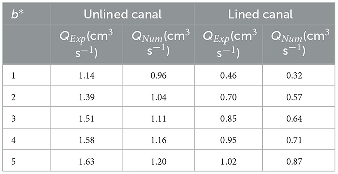
Table 2. Comparison between the estimated seepage losses from physical (QExp) and Slide2 (QNum) models before and after lining process.
The difference between the physical and Slide2 results was due to systematic errors affecting the seepage loss values. These errors could be instrumental (e.g., high water pressure on the bottom and sides of the physical model may cause unsoldering between the tank walls), theoretical (e.g., adding more water at the beginning of the test may increase the initial depth), observational (e.g., the misread of the final depth), and environmental (e.g., some water may evaporate due to temperature instability during the test). Considering the lined canal, the results revealed the effectiveness of the liner in decreasing the seepage loss by an average percentage of 57%. Thus, the Slide2 model showed its ability to calculate the seepage loss from unlined and lined canals.
By trial and error, obtaining the best form of the linear equation developed by the MLR for the seepage loss ratio (q*), Equation 18 is proposed as follows:
Figure 3 shows the comparison between the actual and predicted values using the MLR model. The figure shows that the MLR model yielded an adjusted R2 value of 0.785, and most predicted values exceeded a 20% error rate. Supplementary Figure 5 shows the error distribution between predicted and actual values. The maximum error in the q* ratio was 5.392. The results showed that the MLR had reduced prediction accuracy with a notable error distribution.
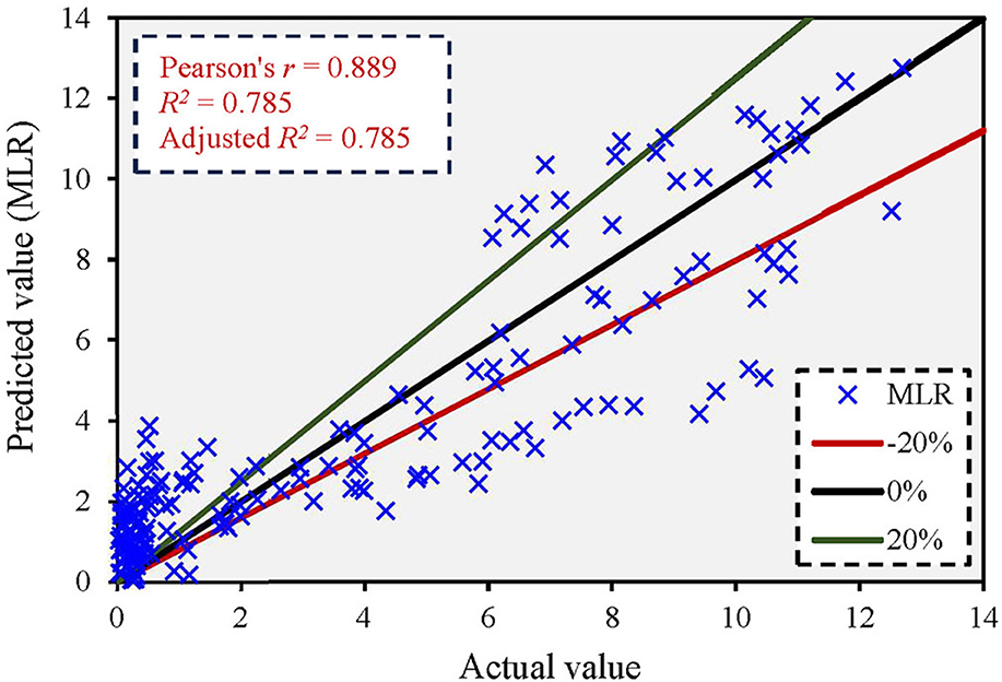
Figure 3. Correlation between actual and predicted values based on the MLR model.
By trial and error, obtaining the best form of the non-linear equation developed by the MNLR for the seepage loss ratio (q*), Equation 19 is proposed as follows:
Figure 4 shows the comparison between the actual and predicted values using the MNLR model. The figure shows that the MNLR model yielded an adjusted R2 value of 0.902, and most of the predicted values exceeded a 20% error rate. Supplementary Figure 6 shows the error distribution between predicted and actual values. The maximum error in the q* ratio was 3.803. The results showed that the MNLR had higher prediction accuracy than the MLR model with low errors.
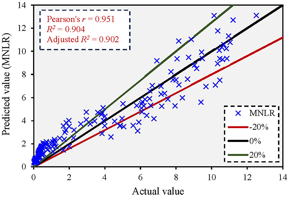
Figure 4. Correlation between actual and predicted values based on the MNLR model.
The developed SVR model used the linear kernel, suggesting a linear relationship between the inputs and the output. However, this kernel was used after trying different kernel types to ensure the best prediction accuracy of the model (Najafzadeh and Anvari, 2023). Figure 5 shows the comparison between the actual and predicted values using the SVR model. The figure shows that the SVR model yielded an adjusted R2 value of 0.745, and most predicted values exceeded a 20% error rate. Supplementary Figure 7 shows the error distribution between predicted and actual values. The maximum error in the q* ratio was 7.255. The results showed that the SVR had a very low prediction accuracy than the MLR and MNLR models with high error distribution.
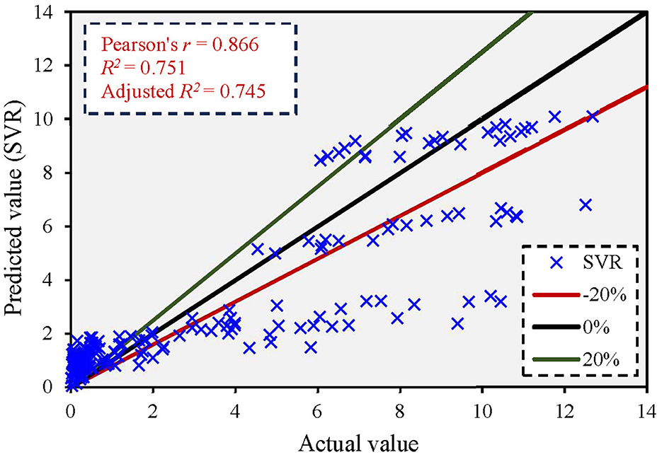
Figure 5. Correlation between actual and predicted values based on the SVR model.
Initially, a single gene and two head lengths were utilized to build the GEP model. During each run, genes and heads were increased by one. Then, the performance of the training and validation datasets was logged. Noticeably, the training and testing stages did not improve considerably for head lengths larger than eight and >3 genes (Najafzadeh et al., 2023). As a result, eight as the head length and three genes per chromosome were chosen. The linking function between three genes was the Addition operator.
After 576,590 generations of testing, there was no significant change in the fitness function and coefficient of determination, suggesting generations can stop. Supplementary Table 2 shows general settings, fitness function, program structure, numerical constants, and genetic operators for developing the GEP model. The trial-and-error method was used to choose all stated parameters to produce the optimal model of the GEP in the form of an algebraic equation between the output variable and input variables. The used function set for the model development was addition (+), subtraction (-), multiplication (*), division (/), square root (Sqrt), cube root (3Rt), quintic root (5Rt), absolute value (Abs), natural logarithm (Ln), Inverse (Inv), addition with three inputs (Add3), division with three inputs (Div3), and division with 4 inputs (Div4).
The developed GEP model for seepage loss estimation from lined canals was expressed analytically in Equation 20 as follows:
Figure 6 shows the comparison between the actual and predicted values using the GEP model. The figure shows that the GEP model yielded an adjusted R2 value of 0.989, and most predicted values were below the 10% error rate. Supplementary Figure 8 shows the error distribution between predicted and actual values. The maximum error in the q*ratio was 1.306. The results revealed that the GEP model had a higher prediction accuracy than the MLR, MNLR, and SVR models, with the lowest error distribution.
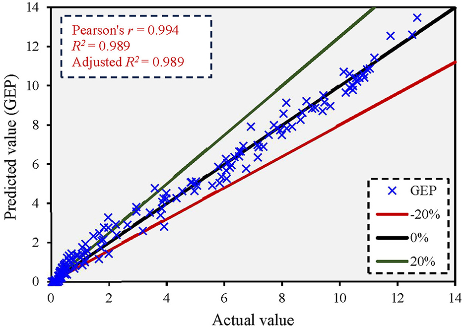
Figure 6. Correlation between actual and predicted values based on the GEP model.
The best ANN architecture was obtained as 4-20-1 after many trials by varying the number of hidden layers and activation functions. This architecture showed that the ANN model had an input layer with 4 nodes (the four input ratios), a hidden layer with 20 nodes, using the sigmoid activation function, and an output layer with 1 node (the output), using the linear activation function. However, these functions were commonly used for regression problems (Haykin, 2009). Moreover, the equation from the developed ANN model for predicting q* ratio was expressed in Equation 21 as follows:
W2= [0.022 −0.043 0.003 0.024 0.020 −0.806 1.138 0.032 0.018 0.042 0.031 −0.017 0.026 −4.283 −2.355 0.014 −2.880 0.082 −0.034 2.814]; B2 = [−2.686]
Where X is the input layer matrix, W1 is the weight matrix of connections between the neurons of the input and hidden layer, B1 is the vector of weights of bias neurons at the hidden layer, W2 is the weight matrix of connections between the hidden and output layer, B2 is the vector of weights of bias neurons at the output layer.
Figure 7 shows the comparison between the actual and predicted values using the ANN model. The figure shows that the ANN model yielded an adjusted R2 value of 0.997, and most predicted values were below the 5% error rate. Supplementary Figure 9 shows the error distribution between predicted and actual values. The maximum error in the q* ratio was 0.709. The results revealed that the ANN model had the highest prediction accuracy compared to the MLR, MNLR, SVR, and GEP models, with the lowest error distribution among them.
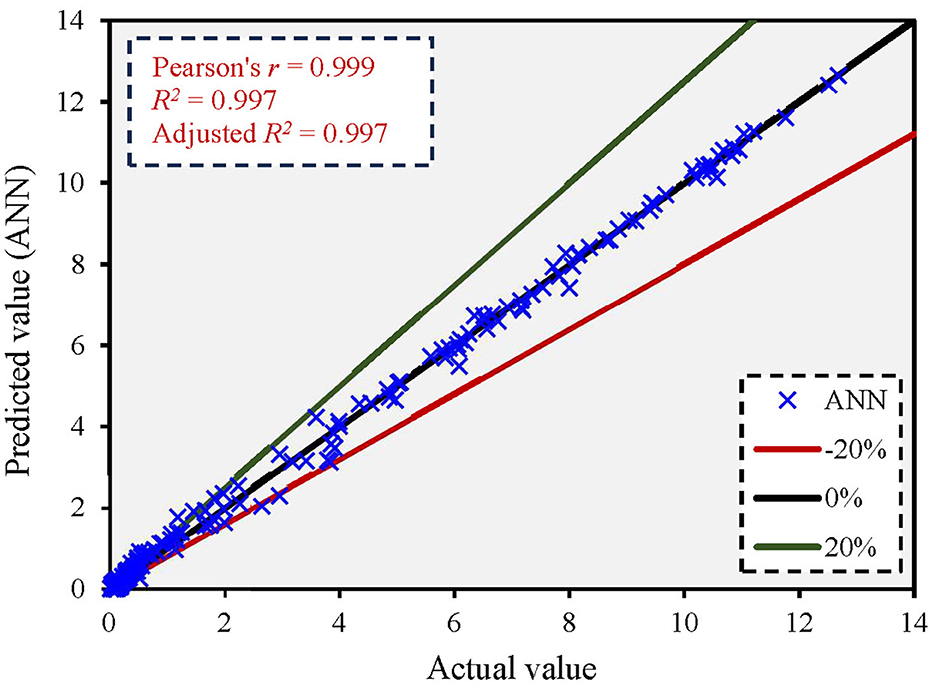
Figure 7. Correlation between actual and predicted values based on the ANN model.
The developed ensemble models had 500 trees obtained from the tuning process, achieving the highest accuracy with low errors. The results of each model were explained in the following sub-sections.
Figure 8 shows the comparison between the actual and predicted values using the AdaBoost model. The figure shows that the AdaBoost model yielded an adjusted R2 value of 0.915, and most predicted values exceeded the 15% error rate. Supplementary Figure 10 shows the error distribution between predicted and actual values. The maximum error in the q*ratio was 3.355. The results revealed that the AdaBoost model had a high prediction accuracy with reasonable error distribution.
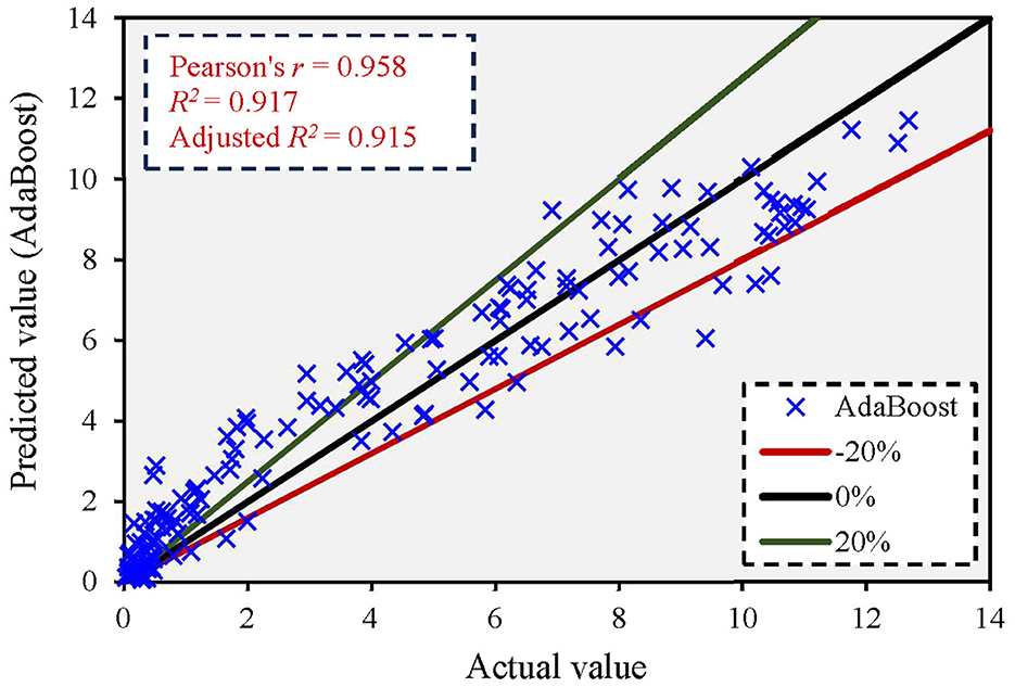
Figure 8. Correlation between actual and predicted values based on the AdaBoost model.
Figure 9 shows the comparison between the actual and predicted values using the RF model. The figure shows that the RF model yielded an adjusted R2 value of 0.986 and most of the predicted values below a 15% error rate. Supplementary Figure 11 shows the error distribution between predicted and actual values. The maximum error in the q* ratio was 1.702. The results revealed that the RF model had a higher prediction accuracy than AdaBoost, with a lower error distribution.
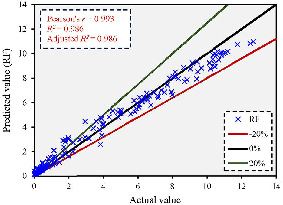
Figure 9. Correlation between actual and predicted values based on the RF model.
Figure 10 shows the comparison between the actual and predicted values using the XGBoost model. The figure shows that the XGBoost model yielded an adjusted R2 value of 0.996 and most of the predicted values below a 5% error rate. Supplementary Figure 12 shows the error distribution between predicted and actual values. The maximum error in the q* ratio was 1.228. The results revealed that the XGBoost model had a higher prediction accuracy than AdaBoost and RF models, with the lowest error distribution among them.

Figure 10. Correlation between actual and predicted values based on the XGBoost model.
Tables 3, 4 show the estimated statistical indices for the studied ML algorithms for the training and testing stages, respectively. The tables show that the ensemble learning models are significantly better at making predictions than the non-ensemble models. The statistical analysis revealed that among the predicted q* ratios, the SVR and XGBoost models register the lowest (0.700) and highest (1.000) R2-value compared to actual values. Out of the eight ML models applied, RMSE values ranged from a minimum of 0.073 (XGBoost) to a maximum of 2.166 (SVR). The MAPE's range during models training was 0.066–2.481. The higher R2 and WI indices for the XGBoost model suggest it outperformed other algorithms during the training stage. Conversely, based on the lowest R2 (0.700) and WI (0.889) indices, the SVR was inferred to be the least effective.
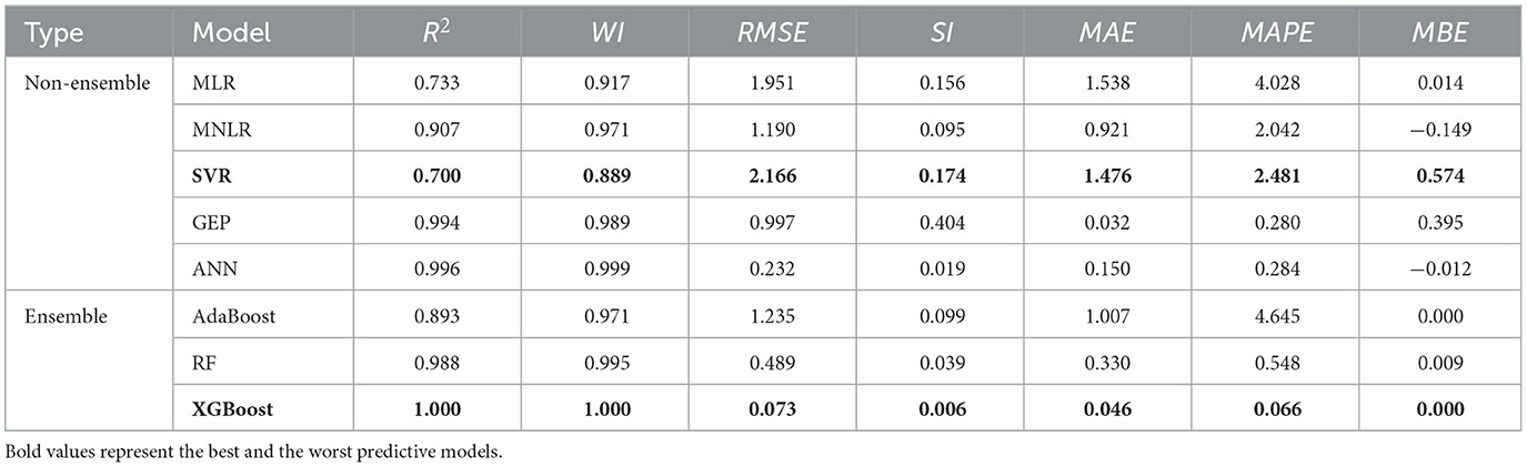
Table 3. Estimated statistical indices of the adopted ML models in the training stage.
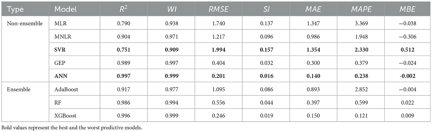
Table 4. Estimated statistical indices of the adopted ML models in the testing stage.
During the testing stage, the descriptive statistics reveal that among the estimated q* ratios, the SVR and ANN models register the lowest (0.751) and highest (0.997) R2-value compared to actual values. Out of the eight models applied, RMSE values ranged from a minimum of 0.201 (ANN) to a maximum of 1.994 (SVR). The MAPE's range during model training was 0.238–2.330. The higher R2 and WI indices for the ANN model suggest it outperformed other algorithms during the testing stage. Conversely, the SVR was also inferred to be the least effective based on the lowest R2 (0.751) and WI (0.909) indices.
Figures 11, 12 present violin box plots of the actual and predicted values of q* during the training and testing stages, respectively. A violin plot is a method of plotting numeric data and can be thought of as a combination of a box plot and a kernel density plot. It shows the distribution of the data across different levels of categorical variables. The “Actual” category likely represents the actual observed values. The plots display the median (central white dot), interquartile range (thick black bar in the center of the violin), and the full range of the data, excluding outliers (thin black lines or “whiskers”). The width of each violin indicates the density of the data at different values, with wider sections representing a higher density (more data points). During both training and testing stages, ensemble models (AdaBoost, RF, and XGBoost) tended to have tighter distributions around lower seepage loss ratios, suggesting more accurate predictions compared to non-ensemble models (MLR, MNLR, SVR, GEP, and ANN).
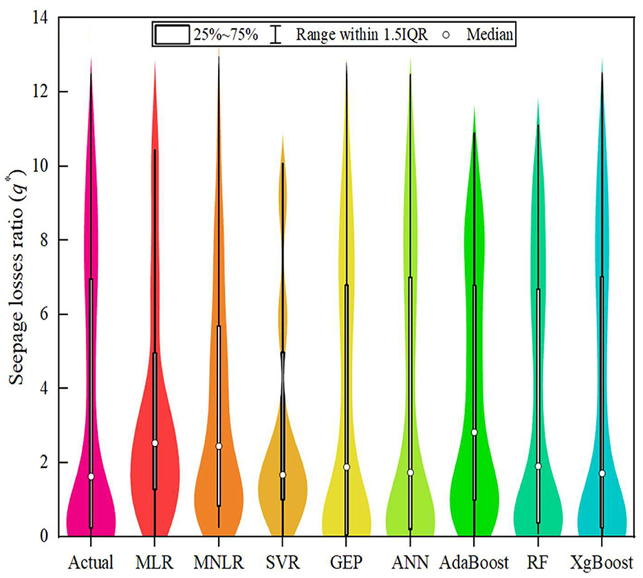
Figure 11. Violin boxplot of the adopted ML models during the training stage.
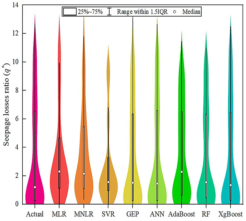
Figure 12. Violin boxplot of the adopted ML models during the testing stage.
In addition, Figures 13, 14 show a comparative analysis of models using the Taylor diagram during the training and testing stages, respectively. Taylor diagrams provide a way of graphically summarizing how closely a pattern matches observations. The diagrams show the correlation coefficient on the azimuthal axis, the standard deviation as the radial distance from the origin, and the centered root mean square difference (RMSD) as the distance from the reference (observed) point. Points closer to the reference point indicate better model performance. Models that are closer to the reference point along the arc with a higher correlation coefficient (toward 1.0) and a smaller distance from the reference (smaller RMSD) are considered to have better performance. During the training stage, the XGBoost and SVR models were found to be the closest and furthest to the actual point, respectively. Consequently, it was indicated that the XGBoost model had performed best among all eight ML models to estimate seepage loss from lined canals. While in the testing stage, the ANN model was the best predictor among all eight ML models.
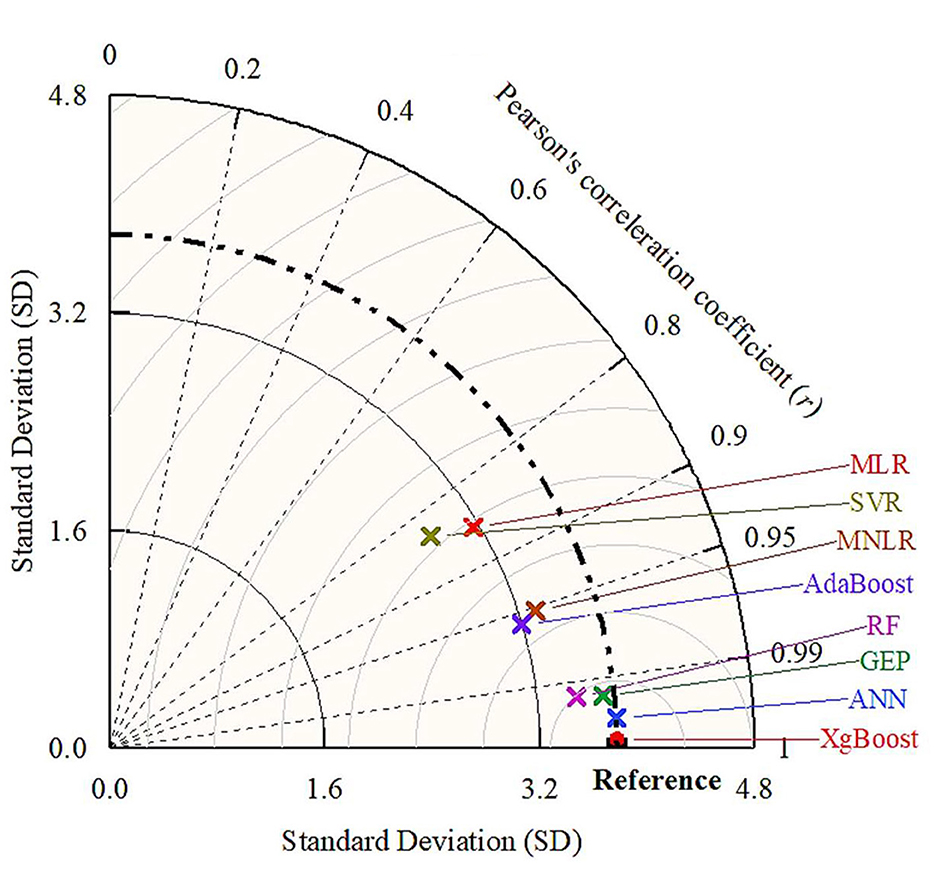
Figure 13. Taylor diagram of the adopted ML models during the training stage.
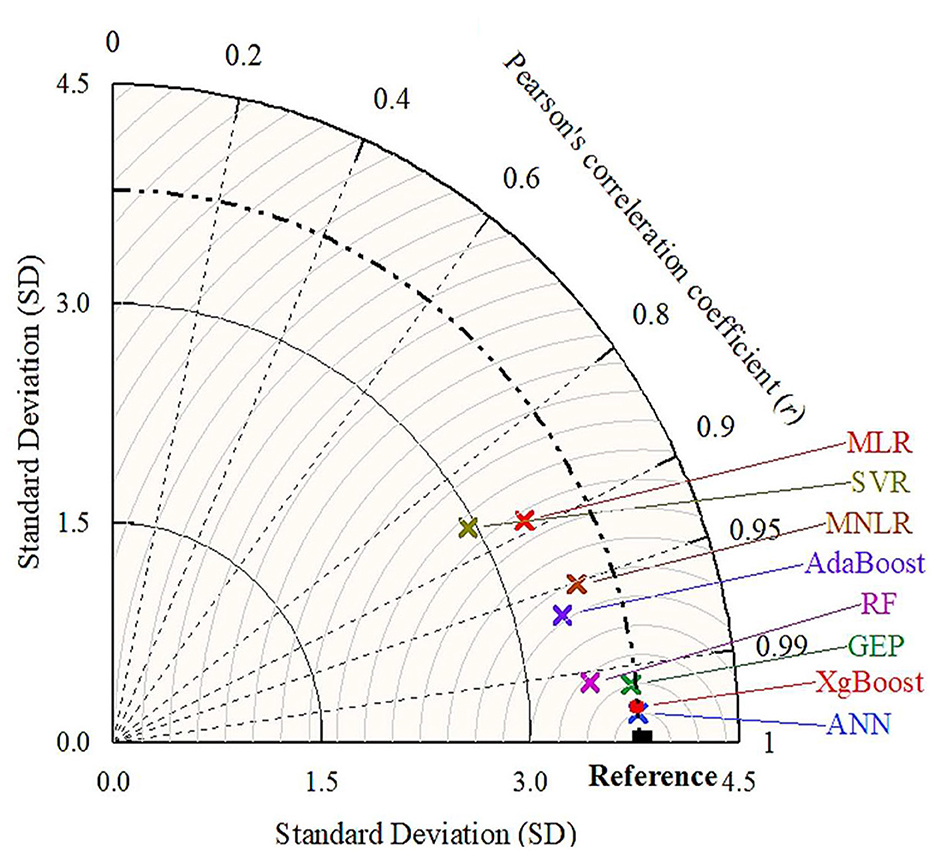
Figure 14. Taylor diagram of the adopted ML models during the testing stage.
Employing the k-fold cross-validation technique reduces the chance of the model overfitting to a specific dataset partition, offering a more accurate assessment of the model's performance. Typically, cross-validation serves as a technique to refine and enhance a model. The motivation for using k-fold cross-validation is to obtain a more precise assessment of the model's efficacy and to reduce the potential for overfitting associated with a single train-test partition. Thus, the results from this cross-validation approach validate the reliability and precision of the examined algorithms.
Supplementary Table 3 shows the R2 values for the adopted ML models across 10 folds. The R2 is a statistical measure that represents the proportion of the variance for a dependent variable that's explained by an independent variable or variables in a regression model. A higher R2 value indicates that the model explains a higher proportion of the variance in the data. Supplementary Table 4 shows the WI values for the adopted ML models across 10 folds. The WI is a standardized index that measures the degree of model prediction error and ranges from 0 (no correlation) to 1 (perfect fit). Similar to Supplementary Table 3, it shows high values close to 1, which indicates good model performance. Ensemble models generally showed higher R2 and WI values, indicating better performance. Also, the results showed that the ANN and GEP models had the highest R2 and WI values among the non-ensemble models.
Supplementary Table 5 shows the RMSE values for the adopted ML models across 10 folds. RMSE is a measure of the differences between values predicted by a model and the values observed. The lower the RMSE, the better the model's performance. Supplementary Table 6 shows the SI values for the adopted ML models across 10 folds. SI is a dimensionless performance indicator, with lower values indicating better model performance. Consistent with previous results, ensemble models generally showed lower RMSE and SI values, indicating better performance.
Supplementary Table 7 shows the MAE values for the adopted ML models across 10 folds. The MAE measures the average magnitude of the errors in a set of predictions without considering their direction. Lower MAE values suggest better model accuracy. Again, ensemble models, particularly XGBoost, tended to have lower MAE values, indicating superior performance. Supplementary Table 8 shows the MAPE values for the adopted ML models across 10 folds. The MAPE expresses the accuracy as a percentage, with lower values indicating higher accuracy. The results show that ensemble models have lower MAPE values compared to non-ensemble models, with XGBoost consistently having the lowest values. Supplementary Table 9 shows the MBE values for the adopted ML models across 10 folds. The MBE measures the average of the residuals (errors) in the predictions. A value close to 0 indicates no bias. The table shows that some models have positive or negative biases, but ensemble models tended to have MBE values closer to zero, suggesting less bias in predictions.
Based on the k-fold cross-validation, a higher performance was detected when employing ensemble models (AdaBoost, RF, and XGBoost) across various performance indices (R2, WI, RMSE, SI, MAE, MAPE, and MBE). XGBoost appeared to be the most consistent top performer with high R2 and WI values, low RMSE, SI, MAE, and MAPE scores, and MBE values close to zero, indicating its strong predictive ability and generalizability. However, The ANN outperforms all models with higher correlation values and lower errors. So, while XGBoost was a strong performer, the ANN model stood out as the top predictor.
To explore the effect of lining on the seepage loss ratio (q*), the ratios of k* and t* were selected to be 0.1 and 0.2, respectively. The k* ratio of 0.1 was chosen because it is neither too low nor too high within the investigated range. Moreover, the effect of lining on seepage loss was slightly reduced at a higher k* ratio ≈ 1. While, at an extremely low ratio of (k*) ≤ 0.01, seepage loss almost vanished. The t* ratio of 0.2 was selected because a thicker liner is typically more effective in reducing seepage loss than a thinner one (t* ratio < 0.2). Moreover, it provides a greater barrier to water flow (Eltarabily et al., 2023a,b).
Supplementary Figure 13A shows the q* values under different k* and b* ratios when the t* ratio equals 0.20 and z equals 1. At a t* ratio of 0.20, seepage losses were reduced by a mean percentage of 8.9, 20.4, 67.9, 82.6, 96.2, 97.4, 99.4, and 99.7% for the k* ratios of 0.50, 0.30, 0.10, 0.05, 0.01, 0.005, 0.005, 0.001, and 0.0005, respectively. Supplementary Figure 13B shows that as t* increases, seepage losses considerably decrease. At the k* ratio of 0.1 and z equals 1, the average percentage of seepage losses was reduced by 10, 23, 41, 61, and 68% for t* ratios of 0.02, 0.05, 0.10, 0.15, and 0.20, respectively.
Supplementary Figure 14A shows the average seepage reduction at each k* ratio corresponding to the investigated z values. It can be noted that as the z-values increase, the q* ratio increases. At t* ratio of 0.20, every increase in the value of z by 0.5 caused a reduction in the mean percentage of seepage losses by 12.1, 23.3, 67.8, 84.5, 96.1, 97.3, 99.3, and 99.7% for the k* ratios of 0.5, 0.3, 0.1, 0.05, 0.01, 0.005, 0.001, and 0.0005, respectively. Supplementary Figure 14B shows the average seepage reduction at each t*ratio corresponding to the investigated z-values. At a k* ratio of 0.10, every increase in the value of z by 0.5 caused a reduction in the mean seepage losses by 9.93, 22.6, 41.4, 61.1, and 67.8% for the t* ratios of 0.02, 0.05, 0.1, 0.15, and 0.2, respectively. Generally, when the side slopes were flat, there was more seepage than when the canal had steep side slopes.
Based on the results of the parametric analysis, the liner hydraulic conductivity positively correlates with the seepage losses. The liner hydraulic conductivity played a crucial role in determining the seepage losses. A liner with high hydraulic conductivity allows more water to pass through it, leading to higher seepage losses. Conversely, a low hydraulic conductivity liner resists seepage flow and reduces seepage losses. Moreover, regardless of the b* ratio, as the k* ratio gets lower and the t* ratio gets higher, the seepage losses decrease at all z-values.
The sensitivity analysis can help to further analyze the data type and explore the importance of each input parameter for the corresponding output. Figure 15 shows the importance of each input parameter. It illustrates that the seepage loss ratio (q*) was affected by 17, 5, 62, and 16% for b*, z, k*, and t*, respectively. Results showed that the q* ratio was highly affected by the k* ratio but was lightly affected by the b* and t* ratios. However, the side slope (z) was the least important to the seepage loss estimation compared to the other investigated parameters. These results concurred with El-Molla and El-Molla (2021b) and Eltarabily et al. (2023a,b).
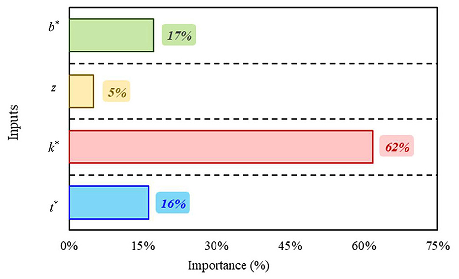
Figure 15. Importance of input parameters for estimating the output (q*).
This study demonstrated effective modeling and prediction of seepage loss from lined irrigation canals using physical and Slide2 models as well as ML techniques. The Slide2 model was calibrated using experimental data and used to generate datasets on seepage loss considering different canal geometries and liner properties. Both non-ensemble and ensemble ML models were developed and evaluated for predicting seepage loss. The non-ensemble models were MLR, MNLR, SVR, GEP, and ANN, whereas the ensemble models included AdaBoost, RF, and XGBoost.
The high concordance between actual and predicted results underscores the efficacy of these models. All developed models, excluding the SVR and MLR models, are identified as highly reliable predictive tools with R2 values exceeding 0.85. The ensemble ML models showcased a pronounced edge, demonstrated by higher R2 values and diminished errors (RMSE, SI, MAE, MAPE, and MBE), suggesting reduced differences between the actual and predicted values. The ANN model was superior among the non-ensemble models, while the SVR model lagged in accuracy. For ensemble models, the XGBoost emerged as the top predictor.
Further evaluation revealed the ANN model as the overall most reliable model, characterized by the highest accuracy and lowest errors. Sensitivity analysis highlighted liner hydraulic conductivity as the crucial parameter influencing seepage loss prediction. In summary, the study effectively demonstrated the dependability of data-driven modeling in delivering quick, cost-effective, and reasonably accurate predictions of seepage loss from lined irrigation canals.
Moreover, this study primarily utilized essential geometric and hydraulic parameters of irrigation canals. By integrating additional parameters such as soil characteristics, liner positions, and groundwater table variations, there is potential to further refine the accuracy and flexibility of the developed models. Although the ANN model demonstrated strong predictive capabilities, more precise field-based validation is recommended, especially for enhancing insights into real-world irrigation canal systems.
The datasets presented in this study can be found in online repositories. The names of the repository/repositories and accession number(s) can be found in the article/Supplementary material.
MGE: Investigation, Methodology, Writing—original draft. HA-E: Conceptualization, Supervision, Writing—review & editing. MZ: Funding acquisition, Project administration, Writing—review & editing. MKE: Data curation, Validation, Visualization, Writing—original draft. ME: Data curation, Software, Validation, Visualization, Writing—review & editing. TS: Investigation, Validation, Writing—review & editing.
The author(s) declare financial support was received for the research, authorship, and/or publication of this article. The Slovak Research and Development Agency supported this work under contract no. APVV-20-0281. This work was supported by project HUSKROUA/1901/8.1/0088, Complex Flood-Control Strategy on the Upper-Tisza catchment area.
The authors would like to express their sincere appreciation and gratitude to the reviewers for their valuable comments.
The authors declare that the research was conducted in the absence of any commercial or financial relationships that could be construed as a potential conflict of interest.
All claims expressed in this article are solely those of the authors and do not necessarily represent those of their affiliated organizations, or those of the publisher, the editors and the reviewers. Any product that may be evaluated in this article, or claim that may be made by its manufacturer, is not guaranteed or endorsed by the publisher.
The Supplementary Material for this article can be found online at: https://www.frontiersin.org/articles/10.3389/frwa.2023.1287357/full#supplementary-material
Abd-Elaty, I., Pugliese, L., Bali, K. M., Grismer, M. E., and Eltarabily, M. G. (2022). Modelling the impact of lining and covering irrigation canals on underlying groundwater stores in the Nile Delta, Egypt. Hydrol. Process. 36, e14466. doi: 10.1002/hyp.14466
Abd-elziz, S., Zelenáková, M., Kršák, B., and Abd-elhamid, H. F. (2022). Spatial and temporal effects of irrigation canals rehabilitation on the land and crop yields, a case study: the Nile Delta, Egypt. Water 14, 50808. doi: 10.3390/w14050808
Aghvami, E., Abbaspour, A., Ghorbani, M. A., and Salmasi, F. (2013). Estimation of channels seepage using SEEP/W and evolutionary polynomial regression (EPR) modeling (case study: Qazvin and Isfahan channels). J. Civ. Eng. Urban. 3, 211–215.
Aljarah, I., Faris, H., and Mirjalili, S. (2018). Optimizing connection weights in neural networks using the whale optimization algorithm. Soft Comput. 22, 1–15. doi: 10.1007/s00500-016-2442-1
Alrefaei, A., Alsaadawi, M. M., and Wagdy, W. (2023). Characteristics of high-strength concrete reinforced with steel fibers recovered from waste tires. Key Eng. Mater. 945, 145–156. doi: 10.4028/p-d5v1nm
Alsaadawi, M. M., Amin, M., and Tahwia, A. M. (2022). Thermal, mechanical and microstructural properties of sustainable concrete incorporating Phase change materials. Constr. Build. Mater. 356, 129300. doi: 10.1016/j.conbuildmat.2022.129300
Archontoulis, S. V., and Miguez, F. E. (2015). Nonlinear regression models and applications in agricultural research. Agron. J. 107, 786–798. doi: 10.2134/agronj.2012.0506
ASTM C185-13 (2013). Standard test method for measurement of rate of absorption of water by hydraulic cement concretes. ASTM Int. 41, 1–6. doi: 10.1520/C1585-13
Bahramlu, R. (2011). Evaluation of leakage losses in irrigated irrigation channels in cold regions and its effect on water resources reserves (case study in Hamadan province). Iran. J. Water Res. 5, 141–150.
Balkhair, K. S. (2002). Aquifer parameters determination for large diameter wells using neural network approach. J. Hydrol. 265, 118–128. doi: 10.1016/S0022-1694(02)00103-8
Carabineanu, A. (2012). Free-boundary seepage from asymmetric soil channels. Int. J. Math. Math. Sci. 2012, 1–14. doi: 10.1155/2012/962963
Chahar, B. R. (2007). Analysis of seepage from polygon channels. J. Hydraul. Eng. 133, 451–460. doi: 10.1061/(ASCE)0733-9429(2007)133:4(451)
Chen, T., and Guestrin, C. (2016). “Xgboost: a scalable tree boosting system,” in Proceedings of the 22nd ACM SIGKDD International Conference on Knowledge Discovery and Data Mining (New York, NY: ACM), 785–794.
Chengsheng, T., Huacheng, L., and Bing, X. (2017). “AdaBoost typical Algorithm and its application research,” in MATEC Web of Conferences (EDP Sciences), 139, 00222. doi: 10.1051/matecconf/201713900222
Christian, S. S., and Trivedi, N. M. (2018). “Seepage through canals”-a review. Int. J. Res. Appl. Sci. Eng. Technol. 6, 865–867.
Deng, L., Hinton, G., and Kingsbury, B. (2013). “New types of deep neural network learning for speech recognition and related applications: an overview,” in 2013 IEEE International Conference on Acoustics, Speech and Signal Processing (IEEE) (Vancouver, CA), 8599–8603.
Dietterich, T. G. (2000). “Ensemble methods in machine learning,” in International Workshop on Multiple Classifier Systems (Cham: Springer), 1–15.
Elkamhawy, E., Zelenakova, M., and Abd-Elaty, I. (2021). Numerical canal seepage loss evaluation for different lining and crack techniques in arid and semi-arid regions: a case study of the river nile, Egypt. Water 13, 35. doi: 10.3390/w13213135
El-Molla, D., and El-Molla, M. (2021b). Reducing the conveyance losses in trapezoidal canals using compacted earth lining. Ain Shams Eng. J. 12, 18. doi: 10.1016/j.asej.2021.01.018
El-Molla, D. A., and El-Molla, M. A. (2021a). Seepage losses from trapezoidal earth canals with an impervious layer under the bed. Water Pract. Technol. 16, 530–540. doi: 10.2166/wpt.2021.010
El-Molla, D. A., and Eltarabily, M. G. (2023). Estimation of seepage losses from cracked rigid canal liners using finite element modeling. J. Appl. Water Eng. Res. 2023, 2233904. doi: 10.1080/23249676.2023.2233904
Elshaarawy, M., Hamed, A. K., and Hamed, S. (2023). Regression-based models for predicting discharge coefficient of triangular side orifice. J. Eng. Res. 7, 224–231. doi: 10.21608/erjeng.2023.244750.1292
Elshaarawy, M. K., and Hamed, A. K. (2023). Predicting discharge coefficient of triangular side orifice using ANN and GEP models. Water Sci. 2023, 2290301. doi: 10.1080/23570008.2023.2290301
Eltarabily, M. G., Elshaarawy, M. K., Elkiki, M., and Selim, T. (2023a). CFD and ANN for modeling lined irrigation canals with low-density polyethylene and cement concrete liners. Irrig. Drain. 2023, 2911. doi: 10.1002/ird.2911
Eltarabily, M. G., Elshaarawy, M. K., Elkiki, M., and Selim, T. (2023b). Modeling surface water and groundwater interactions for seepage losses estimation from unlined and lined canals. Water Sci. 37, 315–328. doi: 10.1080/23570008.2023.2248734
Eltarabily, M. G. A., and Negm, A. M. (2015). Numerical simulation of fertilizers movement in sand and controlling transport process via vertical barriers. Int. J. Environ. Sci. Dev. 6, 559–565. doi: 10.7763/ijesd.2015.v6.657
Evans, J. H. (1972). Dimensional analysis and the Buckingham Pi theorem. Am. J. Phys. 40, 1815–1822. doi: 10.1119/1.1987069
Fallah-Mehdipour, E., Bozorg Haddad, O., and Mariño, M. A. (2013). Prediction and simulation of monthly groundwater levels by genetic programming. J. Hydro-environment Res. 7, 253–260. doi: 10.1016/j.jher.2013.03.005
Ferreira, C. (2001). Gene expression programming: a new adaptive algorithm for solving problems. arXiv Prepr. cs/0102027. doi: 10.48550/arXiv.cs/0102027
Flood, I., and Kartam, N. (1994). Neural networks in civil engineering. II: systems and application. J. Comput. Civ. Eng. 8, 149–162. doi: 10.1061/(asce)0887-3801(1994)8:2(149)
Gad, M., Abdelhaleem, H. M., and OASW. (2023). Forecasting the seepage loss for lined and un-lined canals using artificial neural network and gene expression programming. Geomat. Nat. Hazards Risk 14, 2221775. doi: 10.1080/19475705.2023.2221775
Ghazaw, Y. M. (2011). Design and analysis of a canal section for minimum water loss. Alexandria Eng. J. 50, 337–344. doi: 10.1016/j.aej.2011.12.002
Haykin, S. (2009). Neural Networks and Learning Machines, 3rd Edn. Hamilton: Pearson Education, Inc., McMaster University. Available online at:http://dai.fmph.uniba.sk/courses/NN/haykin.neural-networks.3ed.2009.pdf (accessed June 1, 2023).
Ho, T. K. (1995). “Random decision forests,” in Proceedings of 3rd International Conference on Document Analysis and Recognition (IEEE) (Montreal, QC), 278−282.
Hosseinzadeh Asl, R., Salmasi, F., and Arvanaghi, H. (2020). Numerical investigation on geometric configurations affecting seepage from unlined earthen channels and the comparison with field measurements. Eng. Appl. Comput. Fluid Mech. 14, 236–253. doi: 10.1080/19942060.2019.1706639
Jamel, A. A. J. (2016). Analysis and estimation of downward seepage from lining and unlining triangular open channel. Eng. Technol. J. 34, 406–419. doi: 10.30684/etj.34.2A.18
Kahlown, M. A., and Kemper, W. D. (2005). Reducing water losses from channels using linings: costs and benefits in Pakistan. Agric. Water Manag. 74, 57–76. doi: 10.1016/j.agwat.2004.09.016
Kohavi, R. (1995). “A study of cross-validation and bootstrap for accuracy estimation and model selection,” in IJCAI (Montreal, QC), 1137–1145.
Lallahem, S., Mania, J., Hani, A., and Najjar, Y. (2005). On the use of neural networks to evaluate groundwater levels in fractured media. J. Hydrol. 307, 92–111. doi: 10.1016/j.jhydrol.2004.10.005
Lund, A. A. R., Gates, T. K., and Scalia, J. (2023). Characterization and control of irrigation canal seepage losses: a review and perspective focused on field data. Agric. Water Manag. 289, 108516. doi: 10.1016/j.agwat.2023.108516
Moghazi, H. E. M., and Ismail, E. S. (1997). A study of losses from field channels under arid region conditions. Irrig. Sci. 17, 105–110. doi: 10.1007/s002710050028
Mohanty, S., Jha, M. K., Kumar, A., and Panda, D. K. (2013). Comparative evaluation of numerical model and artificial neural network for simulating groundwater flow in Kathajodi–Surua Inter-basin of Odisha, India. J. Hydrol. 495, 38–51. doi: 10.1016/j.jhydrol.2013.04.041
Mowafy, M. H. (2001). “Seepage losses in Ismailia canal,” in Sixth International Water Technology Conference, IWTC. Alexandria, 195–211.
Najafzadeh, M., Ahmadi-Rad, E. S., and Gebler, D. (2023). Ecological states of watercourses regarding water quality parameters and hydromorphological parameters: deriving empirical equations by machine learning models. Stoch. Environ. Res. Risk Assess. 37, 1–24. doi: 10.1007/s00477-023-02593-z
Najafzadeh, M., and Anvari, S. (2023). Long-lead streamflow forecasting using computational intelligence methods while considering uncertainty issue. Environ. Sci. Pollut. Res. 30, 84474–84490. doi: 10.1007/s11356-023-28236-y
Najafzadeh, M., and Barani, G.-A. (2011). Comparison of group method of data handling based genetic programming and back propagation systems to predict scour depth around bridge piers. Sci. Iran. 18, 1207–1213. doi: 10.1016/j.scient.2011.11.017
Najafzadeh, M., Etemad-Shahidi, A., and Lim, S. Y. (2016). Scour prediction in long contractions using ANFIS and SVM. Ocean Eng. 111, 128–135.
Najafzadeh, M., and Saberi-Movahed, F. (2019). GMDH-GEP to predict free span expansion rates below pipelines under waves. Mar. Georesources Geotechnol. 37, 375–392. doi: 10.1080/1064119X.2018.1443355
Najafzadeh, M., Saberi-Movahed, F., and Sarkamaryan, S. (2018). NF-GMDH-Based self-organized systems to predict bridge pier scour depth under debris flow effects. Mar. Georesources Geotechnol. 36, 589–602. doi: 10.1016/j.oceaneng.2015.10.053
Najafzadeh, M., and Tafarojnoruz, A. (2016). Evaluation of neuro-fuzzy GMDH-based particle swarm optimization to predict longitudinal dispersion coefficient in rivers. Environ. Earth Sci. 75, 1–12. doi: 10.1007/s12665-015-4877-6
Neter, J., Kutner, M. H., Nachtsheim, C. J., and Wasserman, W. (1996). Applied Linear Statistical Models. Homewood, IL: Richard D. Irwin, Inc.
Nourani, V., Sharghi, E., and Aminfar, M. (2012). Integrated ANN model for earthfill dams seepage analysis: Sattarkhan Dam in Iran. Artif. Intell. Res. 1, 22. doi: 10.5430/air.v1n2p22
Osman, M. A., and Rahman, B. A. A. (2008). Investigation of seepage flow through irrigation canal founded on soil of infinite depth. Sudan Eng. Soc. J. 54, 57–67.
Rocscience (2002). Groundwater Module in Slide 2D Finite Element Program for Groundwater Analysis. Toronto.
Saberi-Movahed, F., Najafzadeh, M., and Mehrpooya, A. (2020). Receiving more accurate predictions for longitudinal dispersion coefficients in water pipelines: training group method of data handling using extreme learning machine conceptions. Water Resour. Manag. 34, 529–561. doi: 10.1007/s11269-019-02463-w
Saha, B. (2015). A critical study of water loss in canals and its reduction measures. Int. J. Eng. Res. Appl. 5, 53–56.
Salmasi, F., and Abraham, J. (2020). Predicting seepage from unlined earthen channels using the finite element method and multi variable nonlinear regression. Agric. Water Manag. 234, 106148. doi: 10.1016/j.agwat.2020.106148
Samani, N., Gohari-Moghadam, M., and Safavi, A. A. (2007). A simple neural network model for the determination of aquifer parameters. J. Hydrol. 340, 1–11. doi: 10.1016/j.jhydrol.2007.03.017
Schmidhuber, J. (2015). Deep learning in neural networks: an overview. Neural Netw. 61, 85–117. doi: 10.1016/j.neunet.2014.09.003
Selim, T., Kamal, A., Mohamed, H., and Eltarabily, M. G. (2023). Numerical investigation of flow characteristics and energy dissipation over piano key and trapezoidal labyrinth weirs under free - flow conditions. Model. Earth Syst. Environ. 23, 1844. doi: 10.1007/s40808-023-01844-w
Sharief S. M. V. and Zakwan M. (2021). Comparative analysis of seepage loss through different canal linings. Int. J. Hydrol. Sci. Technol. 1, 1. doi: 10.1504/ijhst.2021.10037172
Sharma, H. D., and Chawla, A. S. (1979). Canal seepage with boundary at finite depth. J. Hydraul. Div. 105, 877–897.
Swamee, P. K., Mishra, G. C., and Chahar, B. R. (2000). Design of minimum seepage loss canal sections. J. Irrig. Drain. Eng. 126, 28–32. doi: 10.1061/(asce)0733-9437(2000)126:1(28)
Taormina, R., Chau, K., and Sethi, R. (2012). Artificial neural network simulation of hourly groundwater levels in a coastal aquifer system of the Venice lagoon. Eng. Appl. Artif. Intell. 25, 1670–1676. doi: 10.1016/j.engappai.2012.02.009
Uchdadiya, K. D., and Patel, J. N. (2014). Seepage losses through unlined and lined canals. Int. J. Adv. Appl. Math. Mech. 2, 88–91.
Verma, J. P. (2012). Data Analysis in Management With SPSS Software. Cham: Springer Science & Business Media.
Vishnoi, R. P., and Saxena, R. (2014). Determination of seepage losses in unlined channels. Int. J. Comput. Appl. 975, 8887.
Whigham, P. A., and Crapper, P. F. (2001). Modelling rainfall-runoff using genetic programming. Math. Comput. Model. 33, 707–721. doi: 10.1016/S0895-7177(00)00274-0
Whitley, D., Starkweather, T., and Bogart, C. (1990). Genetic algorithms and neural networks: optimizing connections and connectivity. Parallel Comput. 14, 347–361.
Keywords: ensemble model, irrigation canal, lining, non-ensemble model, prediction, regression, seepage loss
Citation: Eltarabily MG, Abd-Elhamid HF, Zeleňáková M, Elshaarawy MK, Elkiki M and Selim T (2023) Predicting seepage losses from lined irrigation canals using machine learning models. Front. Water 5:1287357. doi: 10.3389/frwa.2023.1287357
Received: 01 September 2023; Accepted: 04 December 2023;
Published: 21 December 2023.
Edited by:
Abbas Roozbahani, Norwegian University of Life Sciences, NorwayReviewed by:
Mohammad Najafzadeh, Graduate University of Advanced Technology, IranCopyright © 2023 Eltarabily, Abd-Elhamid, Zeleňáková, Elshaarawy, Elkiki and Selim. This is an open-access article distributed under the terms of the Creative Commons Attribution License (CC BY). The use, distribution or reproduction in other forums is permitted, provided the original author(s) and the copyright owner(s) are credited and that the original publication in this journal is cited, in accordance with accepted academic practice. No use, distribution or reproduction is permitted which does not comply with these terms.
*Correspondence: Martina Zeleňáková, bWFydGluYS56ZWxlbmFrb3ZhQHR1a2Uuc2s=
Disclaimer: All claims expressed in this article are solely those of the authors and do not necessarily represent those of their affiliated organizations, or those of the publisher, the editors and the reviewers. Any product that may be evaluated in this article or claim that may be made by its manufacturer is not guaranteed or endorsed by the publisher.
Research integrity at Frontiers
Learn more about the work of our research integrity team to safeguard the quality of each article we publish.