
94% of researchers rate our articles as excellent or good
Learn more about the work of our research integrity team to safeguard the quality of each article we publish.
Find out more
ORIGINAL RESEARCH article
Front. Water , 06 October 2023
Sec. Water Resource Management
Volume 5 - 2023 | https://doi.org/10.3389/frwa.2023.1268593
 Aboubakar Gasirabo1,2,3
 Chen Xi1,2*Alishir Kurban1,2Tie Liu1,2Hamad R. Baligira3,4Jeanine Umuhoza1,2,3Adeline Umugwaneza1,2,3Umwali Dufatanye Edovia1,2,3
The Nile Nyabarongo, which is Rwanda's largest river, is facing stress from both human activities and climate change. These factors have a substantial contribution to the water processes, making it difficult to effectively manage water resources. To address this issue, it is important to find out the most accurate techniques for simulating hydrological processes. This study aimed to calibrate the SWAT model employing various algorithms such as GLUE, ParaSol, and SUFI-2 for the simulation of hydrology in the basin of the Nile Nyabarongo River. Different data sources, such as DEM, Landsat images, soil data, and daily meteorological data, were utilized to input information into the SWAT modeling process. To divide the basin area effectively, 25 sub-basins were created, with due consideration of soil characteristics and the diverse land cover. The outcomes point out that SUFI-2 outperformed the other algorithms for SWAT calibration, requiring fewer computing model runs and producing the best results. ParaSol established residing the least effective algorithm. After calibration with SUFI-2, the most sensitive parameters for modeling were revealed to be (1) the Effective Channel Hydraulic Conductivity (CH K2) measuring how well water can flow through a channel, with higher values indicating better conductivity, (2) Manning's n value (CH N2) representing the roughness or resistance to flow within the channel, with smaller values suggesting a smoother channel, (3) Surface Runoff Lag Time (SURLAG) quantifying the delay between rainfall and the occurrence of surface runoff, with shorter values indicating faster runoff response, (4) the Universal Soil-Loss Equation (USLE P) estimating the amount of soil loss. The average evapotranspiration within the basin was calculated to be 559.5 mma-1. These calibration results are important for decision-making and updating policies related to water balance management in the basin.
In the boundaries of the Nile Nyabarongo River Basin, there are significant challenges related to unexpected occurrences of flood alongside the erosion of soil caused by land and climate characteristics (Uwacu et al., 2021). This degradation of the soil negatively affects agriculture in the region, particularly in drylands where unsustainable intense rainfall and land use contribute to erosion and soil loss (Kabirigi et al., 2017; Rutebuka et al., 2019). Basin operators must have a precise comprehension of soil loss and surface water outflow in sequence to properly control and secure natural resources, especially soil, and water (Kuria et al., 2019). Integrated hydrological models with a process-based approach emerged to be essential appliances for managing water resources and environmental challenges, enabling the examination of the impacts resulting from changes in the boundaries within nature and human activities on various ecosystems (Wolka et al., 2018; Ma and Sb, 2020). The current calibration approaches primarily focus on refining outcomes while refining the models' depiction of these tasks. It has been observed that calibration with single hydrological variables may not accurately simulate additional outward and sub-surface hydrological instabilities (Adams, 2017). To improve the process representation, it is necessary to employ effective calibration techniques that utilize simultaneously measurable basin indicates and sensitive information (Bagheri et al., 2020). However, uncertainties in input data, model structure, and parameters pose challenges to detailed calibration and estimate of hydrological processes in basin models. Some studies suggest that incorporating streamflow, rainfall, and soil moisture data can enhance rainfall-runoff modeling. Wasko and Nathan (2019) have noted that using a particular hydrological indicator for calibration may not provide an accurate representation of other surface- and sub-surface-level hydrological instabilities (Giordan et al., 2020). The latter can be done by applying the combined use of delicate data and measurable hydrological indicators for efficient calibration procedures that enhance model demonstration of the approach (Baird and Low, 2022). Nevertheless, the accurate calibration and estimation of hydrological processes in a basin design is restricted by the input data, model framework, and variables (Zuecco et al., 2016). Various methods are used for hydrological modeling, including the Water Evaluation and Planning (WEAP) system, Agricultural Non-Point Source Pollution (AGNPS) system, and Soil and Water Assessment Tool (SWAT) (Yuan et al., 2020). Among these, the SWAT model, established by the United States Department of Agriculture (USDA) Agricultural Research Service (ARS), is frequently used for estimating hydrological and sediment yields (Liu et al., 2016; Fard and Sarjoughian, 2021). It distributes a geographically appropriate and consistent framework to estimate how different methods for managing land will affect runoff, soil loss, and crop production (Martínez-Mena et al., 2020). The procedure and the alignment of the SWAT model's calibration are essential to modify parameters that influence its outputs (Zhang et al., 2009). Numerous parameters related to soil disintegration, runoff, and water quality need to be calibrated to ensure accurate hydrological modeling using SWAT (Akoko et al., 2021). However, this calibration process encounters uncertainties that require careful consideration. The various techniques and algorithms were initially established for SWAT uncertainty and calibration analysis, including sequential uncertainty fitting Version 2 (SUFI-2), SWAT-CUP, cloud computing infrastructure, artificial neural network (ANN), particle swarm optimization (PSO), generalized likelihood uncertainty estimation (GLUE), parallel solution (ParaSol), genetic algorithms, and Bayesian models, Mengistu et al. (2019) previous studies have utilized these algorithms to calibrate and validate the SWAT model in different basins. The SUFI-2 algorithm has shown to be effective throughout the SWAT model's validation and calibration in the Kunthipuzha basin, while other approaches have been used in data-scarce semi-arid basins in South Africa (Mengistu et al., 2019). Additionally, the study conducted a comprehensive validation and calibration of the SWAT model using multiple variables and sites in a vast mountainous basin defined by considerable spatial alterations. Furthermore, Radcliffe and Mukundan (2017) specifically examined the implications of using CFSR and PRISM precipitation data on the process of calibrating and validating SWAT models, ensuring a rigorous analysis. Abbaspour et al. (2004) and Kumar et al. (2017) used the SUFI-2 technique to calibrate, validate and analyze uncertainties of SWAT for streamflow modeling while Khatun et al. (2018) used the SWAT-CUP to replicate the surface runoff. Singh et al. (2012) applied the cloud approaches for calibration of the SWAT model whereas the ANN was utilized by Jahani et al. (2019) and Pradhan et al. (2020) to evaluate SWAT for hydrologic simulation. Moreover, exploited algorithms based on genetics and Bayesian model to calibrate and assess SWAT model uncertainties (Zhang et al., 2009). Akbari et al. (2022) modeled the runoff management strategies under climate change scenarios using hydrological simulation. They found that runoff decreased by 6–23% and 9–52% for the near and far future, respectively, under the BAU scenario compared to the baseline period. Antithetically, it increased by 3.5–21 and 13–55% for the near and far future periods, respectively, based on the CCP strategy estimated up to 30% higher than the BAU strategy. Moreover, Rahvareh et al. (2023) assessed the climate change impacts on the watershed-scale optimal crop pattern using a set of methods. Their results exhibited that irreparable damage to groundwater depletion is reduced in the optimum state, and lower stress is imposed on the aquifer under the climate change impacts by executing the optimum crop pattern. These techniques have been used in earlier studies to calibrate and validate the SWAT model in several basins.
In the process of utilizing these approaches, it is fundamental to persistently modify the parameters until the predicted effects and the experimental data are logically consistent. It's challenging to choose the appropriate algorithm for calibrating SWAT outputs from all these options. This study, therefore, applied SUFI-2, GLUE, and ParaSol, to (1) evaluate the SWAT model's application in simulating hydrological processes such as sediment yield and runoff, (2) compare and unveil the greatest calibration algorithm following the results of the tests conducted in the Nile Nyabarongo River basin. Overall, this study aims to compare different calibration approaches for the SWAT model to improve its accuracy in the Nile Nyabarongo River Basin. By calibrating parameters using assessed estimates and measured estimations, it will be possible to augment the model's ability to forecast the outcomes of evapotranspiration, runoff, and other related variables.
From an extensive literature review, it was evident that existing studies on hydrologic processes are still deficient in developing countries where the effects of climate variation on hydrological processes have not been fully and appropriately understood (Khaddor et al., 2019). Similarly, this specific subject captured less attention in Rwanda owing to different difficulties, among which, the paucity of ground-based weather recordings both in space and time remains challenging. This situation adds to the intricacy of understanding the complex relationships between rainfall and hydrological processes in the area. Consequently, alarming flash flood incidences are recorded in the area, where the Nyabarongo catchment is the most affected, as a result of rapid hydrological responses right after prolonged heavy rainfall (Gatwaza, 2016). Studies have been conducted in the study area with full attention on the perceptions of local people on the use of Nyabarongo River wetland and its conservation in Rwanda (Nsengimana et al., 2017). Moreover, a very recent study assessed the hydrological response to rainfall events giving much focus on the simulation of discharged flow and volume (Mind'je et al., 2021). However, to the best of our knowledge after an in-depth review of literature, no study has so far evaluated the currently most applied model (SWAT model); which has proved a high level of accuracy in simulating different hydrological processes. In addition, this study has also considered to compare concurrent methods for this model calibration and validation, which is indeed understudied and not explored in the study area. Recap that, the study area is the largest at national level well-known to directly respond to a slight variation in its climatic and land surface characteristics. Therefore, this research comes to complement the existing few studies by bridging the identified gap in previously mentioned literature and provide valuable insights that can guide decision-making and policy updates to better manage water balance components in the basin.
The current modeling was established on elevation data, LULC data, soil data, and daily meteorological datasets (rainfall and flow). To accurately map the dimension of the basin area for the Nyabarongo River, we employed elevation information mined from a 30-meter resolution Digital Elevation Model (DEM) acquired from the Shuttle Radar Topographic Mission (SRTM). This particular DEM dataset was compiled by the National Aeronautics and Space Administration (NASA) www.dwtkns.com/srtm 30m. The elevation of the Nyabarongo basin ranges from 1,342 m to 4,443 m (Figure 1). The geographical area in question encompasses a hilly terrain characterized by sharp inclines found within the volcanic area to the north and along the Congo-Nile split to the west. The Nyabarongo basin's nature displays a rugged landscape featuring steep hills interspersed by deep valleys. In the eastern part, the slopes are more gradual, and there is a large valley downstream where flooding has become a significant concern in recent years (Yamashita et al., 2015). Additionally, soil properties and, LULC play a crucial role in modeling hydrological processes, particularly in simulating runoff for this study. To obtain LULC classes for the basin, we processed satellite imagery (Landsat 8 OLI) acquired from the United States Geological Survey (USGS) EROS data and conducted a supervised classification using the Maximum Likelihood Classification method. We used ArcGIS 10.8 to extract soil property information from a raster file containing global soil types. The soil properties map was carefully created using data obtained from the World Harmonized Soil Database (HWSD) (Alawamy et al., 2020). We identified six LULC classes, including forestland, grassland, built-up areas, wetland, and water bodies (Table 1). In numerous areas in Rwanda, agriculture dependent on rainfall is the main economic pursuit in the Nile Nyabarongo basin, while sizable portions of the basin are covered by forests and grasslands, predominantly on hill summits. The areas of urbanization are substantial as the basin includes a significant portion of the capital city, Kigali, along with other major cities of Rwanda like Muhanga., Huye, and Musanze (Price, 2019).
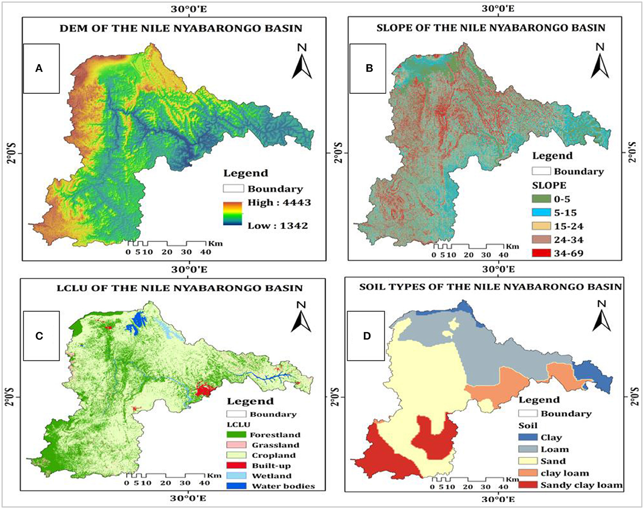
Figure 1. (A) Elevation (in meters), (B) Slope (in %), (C) LCLU (in meter), and (D) Soil types of the Nile Nyabarongo Basin.
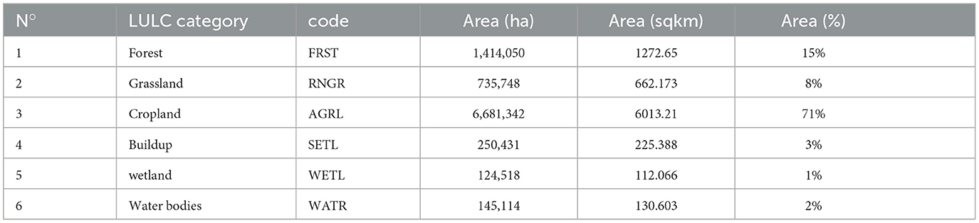
Table 1. Land use land cover classes with total area distribution.
In comparison to the highland region of Rwanda, the soil properties in this area are comparatively younger and naturally more nutrient-rich (Mashingaidze et al., 2020). The identified soil types include clay, loam, sand, clay loam, sand clay, and sandy clay loam (as shown in Figure 1).
To gather meteorological information, data on daily rainfall, and temperature, were obtained from the Rwanda meteorological agency for 34 years (Table 2). The distribution of precipitation in Rwanda is symmetrical, as stated on the official website of the Rwanda Meteorological Agency (www.meteorwanda.gov.rw). This distribution is primarily influenced by the Inter-Tropical Convergence Zone due to the country's high elevation. In the research area, the typical yearly precipitation is slightly above 1,200 mm, which occurs during two distinct rainy seasons. The long rains season takes place from March to May, contributing to approximately half of the total annual rainfall, while the short rains season occurs from September to December (Fuka et al., 2016). Within the research area, the temperature typically falls between the range of 17 to 20°C, and the way temperature and rainfall are dispersed across the area fluctuates due to the topography features of the basin (Kwisanga, 2017; Nsengiyumva and Valentino, 2020). Meteorological data were collected from three different stations located within or near the Nile Nyabarongo basin (Water and Lead, 2017). For the climate data, we considered daily precipitation in millimeters, as well as the mean, minimum, and maximum temperature in degrees Celsius (Neitsch et al., 2011). Due to the historical civil war and genocide in Rwanda, the meteorological records are incomplete, with significant gaps in the data. However, the Kanombe station provided nearly complete and continuous records. Therefore, it was selected as the reference rain gauge to fill in the missing data from other rainfall gauges in the study area for the period from 1982 to 2016 (Irankunda et al., 2022).
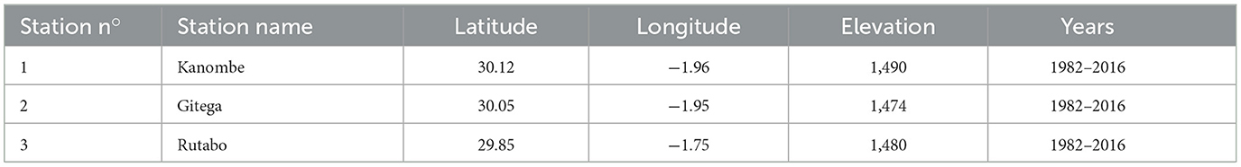
Table 2. Spatial information of meteorological stations.
Rwanda is a country in East Africa that is surrounded by land on all sides situated on the eastern side of Africa's Kivu-Tanganyika rift. It spans an area of 26,338 km2 and is confined by the D.R.Congo, Uganda, Burundi, and Tanzania (Karamage et al., 2016; Nsengiyumva and Valentino, 2020). The basin of the Nyabarongo River has its location in Rwanda and is known as the source of the Nile River. This basin comprises of three sub-basins, namely the Mukungwa sub-basin in the northern region, the Nyabarongo upstream sub-basin in the southern region, and the Nyabarongo downstream sub-basin in the eastern region. Together, these sub-basins play a significant role in Rwanda's drainage system. With an area of 8441.21 km2, In Rwanda, the Nyabarongo River stands as the country's largest river. It stretches ~300 km to Lakeside Rweru from its origins in the west near the boundary with Burundi in southeastern Rwanda. The river's main channel is formed by the Akanyaru River, The Nyabarongo River originates from the elevated landscapes of the Nyungwe National Park, located on the border between the Congo and Nile regions. As it advances east, the river passes through lowland basins and small lakes in the Bugesera-Gisaka swamps in southern Rwanda. Its course is influenced by various smaller rivers, such as the Marenge and Rusine rivers, as well as urbanized areas in Kigali, including Mpazi, Rwanzekuma, Ruganwa, and Yanze rivers, which all contribute to its volume (Nsengiyumva and Valentino, 2020; Omara et al., 2020) (Figure 2).
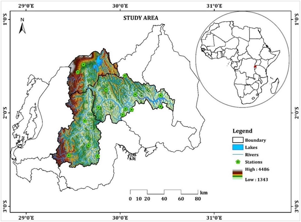
Figure 2. Placement of the research area near the reservoirs of water, river, Meteo stations and the elevation added.
The SWAT is a hydrological simulation designed by the US Department of Agriculture's Agricultural Research Service (ARS). This model is designed to model the manners of water resources using a daily time step. It is based on physical principles and incorporates dynamic elements to accurately represent the behavior of these resources (Neitsch et al., 2011). According to Neitsch et al. (2011), SWAT proves to be highly beneficial when it comes to examining agricultural regions and extensive basins that exhibit diverse soil types, land cover, and management approaches. Its successful adoption can be attributed to the availability of detailed documentation, including theoretical manuals and online tutorials (Heuvelmans et al., 2005; Neitsch et al., 2011; Arnold et al., 2012) as well as additional publications, GIS plug-ins, and support from the development team (Figure 3).
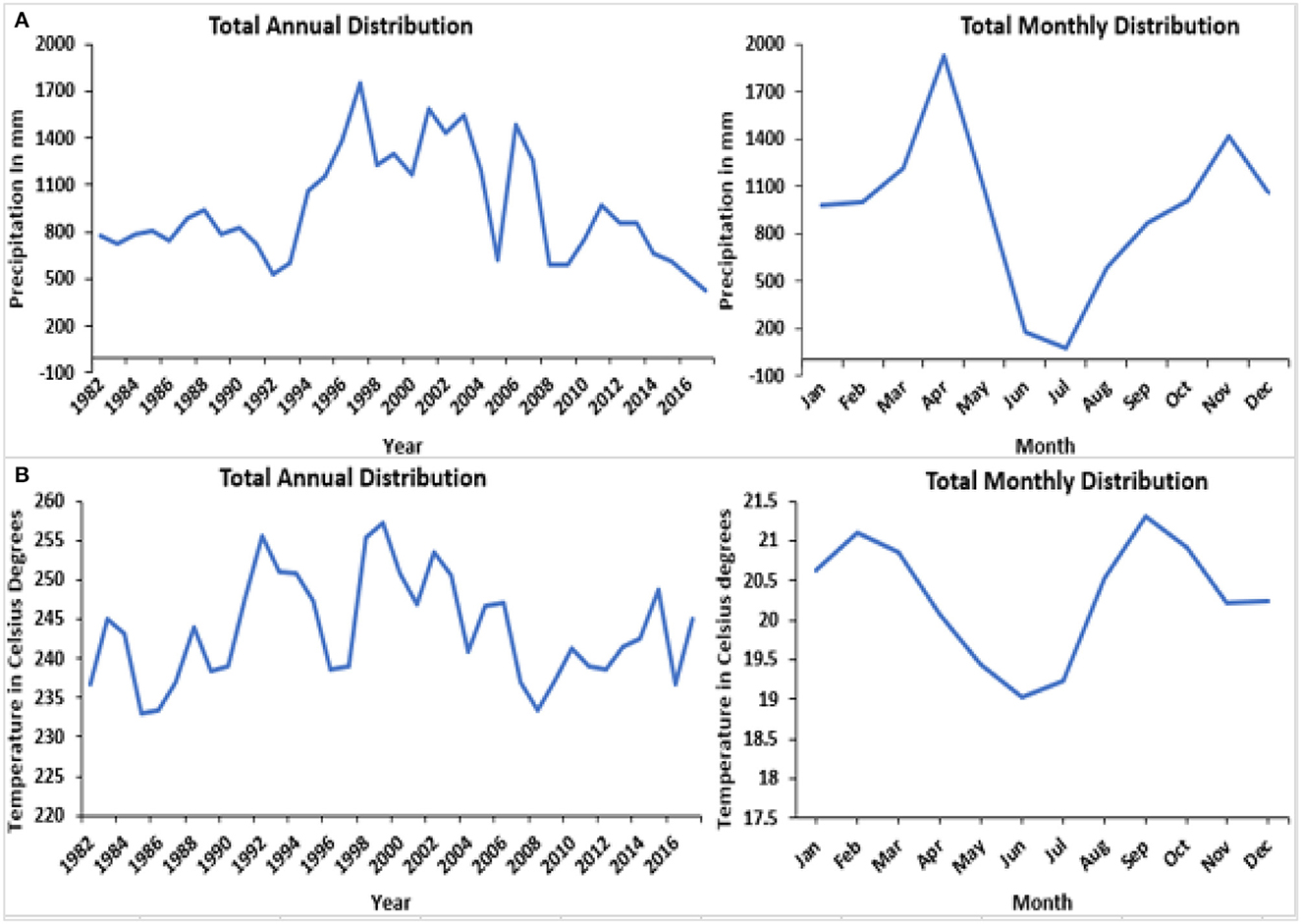
Figure 3. (A) Average annual and monthly precipitation distribution, (B) Average annual and monthly temperature distribution.
The hydrological cycle of a sub-basin is simulated in SWAT using the water balance equation below.
where TWt is the final soil water content; TWo is the initial soil water content (mm); t is time; Rday is the total quantity of precipitation; Msurf is the total quantity of surface runoff; Ea is the total quantity of evapotranspiration; Wseep is the total quantity of percolation flow exiting the soil, and Mgw is the amount of return flow.
SWAT simulates the hydrological cycle of a sub-basin using a water balance equation. The model presents two options for calculating surface runoff: the SCS curve number method (Boughton, 1989) and an additional method (Ogden and Saghafian, 1997). In this research, we utilized SWAT 2012 for hydrological modeling and employed ArcGIS 10.8 software with the Arc SWAT extension. Using the river basin's distinct soil properties, LULC, and elevation, sub-basins were split into Hydrologic Response Units. The HRU serves as the unit for determining hydrologic characteristics, with the water budget driving the simulation. The modeling process incorporates two phases: an in-stream phase, where the model calculates basin loadings from each sub-basin along the stream network, and a land phase, where SWAT simulates the flow, sediment, and nutrient contributions from each HRU, which are then aggregated at the sub-basin level (Shivhare et al., 2018).
SUFI-2 is a probabilistic algorithmic approach commonly used by scientists to assess uncertainty (Kumar et al., 2017). It evaluates both efficiency and parameter uncertainty. The measure of uncertainty in efficiency is determined in accordance with the 95PPU (95 percent accuracy of predictions band), which is calculated in accordance with the cumulative distribution of output variables in SUFI-2 at the 2.5 percent and 97.5 percent thresholds. Parameter uncertainty is captured by utilizing a parametric basis function within a parameter hypercube (Wu et al., 2019). To establish the calibration efficiency, we employ the R-factor, which is determined by scaling the measured data's standard deviation by the 95PPU band's average width. The P-factor represents the percentage of simulations that accurately match the observed data, ranging from 0 to 100 percent, while the R-factor can range from 0 to infinity. When a simulation yields a P-factor of 1 and an R-factor of 0, it signifies a complete alignment with the observed data. SUFI-2, akin to GLUE (Generalized Likelihood Uncertainty Estimation), encompasses all forms of uncertainty by considering parameter uncertainty within the hydrological model. In this research, we employed SWAT-CUP to combine the simulated values from SWAT 2012 with observed data for uncertainty analysis and calibration using the SUFI-2 algorithm (Wu and Chen, 2015). The SUFI-2 technique is as follows:
In the first phase, the goal function (gi) is considered. Next, the minimum and maximum absolute ranges (θj) of the physically significant parameters being optimized are defined.
In the second phase, the preliminary uncertainty estimates are restricted to the parameters for the first round of Latin hypercube testing after a sensitivity assessment for each of the parameters is performed.
In the third phase, Latin hypercube testing is performed, and the equivalent objective functions are assessed. The sensitivity matrix Jij and the following formulas are used to calculate the correlation grid C parameter:
where Cm is the total count of rows in the sensitivity matrix, and p is the total count of parameters to be estimated?
where is the variance of the coefficients of the desired functional resulting from the m model runs?
In the fourth step, the 95PPU is identified. The p-factor (the percent of observations bracketed by the 95PPU) and the r-factor, respectively, are then evaluated:
where and indicate the 95PPU's upper and lower boundaries, and threatens to indicate the observed data's standard deviation.
ParaSol is a revised sort of the UA-SCE global optimization method that aims to incorporate estimate uncertainty during a mechanism of analysis through simulations. ParaSol utilizes the comprehensive exploring space for attributes of UA-SCE, focusing on layouts that are close to optimal (Kan et al., 2017). ParaSol follows the following procedure:
1. The reconstructions are divided into “boundless” and “not boundless” depending on the limit's evaluation of the objective function, similar to GLUE. The application of the revised UA-SCE is accelerated, increasing the range of parameters exploration. This results in separate sets of “boundless” and “not boundless” parameters.
2. Uncertainty prediction is generated by assigning appropriate weights to each “boundless” reconstruction. The regression's sum of squares, referred to as ParaSol (SSQ), is used as the target work:
The correlation between SSQ and NS is:
where represents a set rate for certain observations. All ParaSol objective function values are converted to NS for better comparison with GLUE. ParaSol primarily accounts for parameter uncertainty based on x2-statistics and assumes consistent variability. For comparison purposes, the same sensitivity as GLUE is employed, referred to as “enhanced ParaSol (Zhao et al., 2018).
GLUE is employed to address non-uniqueness of parameter sets across model parameters and scenarios (Zhao et al., 2018). This approach acknowledges that no specific parameter arrangement substantially enhances the goodness-of-fit criterion for over-parameterized models. GLUE consideration throughout potential parameter uncertainty. The estimation of probabilities linked to a parameter set consideration throughout potential sources of error and the influences of parameter covariation on the performance of the model (Zhang et al., 2016). An analysis using the GLUE methodology consists of three primary stages:
1. The “generalized likelihood measure” H(∅), is defined, and a majority of parameter sets are haphazardly selected from the probability distributions. Each set is classified as “behavioral” or “non-behavioral” due to a comparison with a predefined threshold.
2. Each set of behavioral parameters is assigned a “likelihood weight, Ri, due to the subsequent formula:
where n is the number of interactive parameters sets.
3. Finally, the estimated uncertainty is represented as a forecast quintile derived from the aggregated distribution of weighted behavioral parameter sets. The Nash-Sutcliffe coefficient of efficiency (NSE) is commonly used as the likelihood measure for GLUE.
In this context, n corresponds to the total count of recorded data points and the variables yti and symbolize the observed data and the model's simulated output using parameters ∅ at a time ti, respectively, and y denotes the mean value of the annotations.
For more information on the SWAT-CUP, ParaSol, SUFI-2 and GLUE model components, you can look up the SWATCUP instruction request by Abbaspour (2014) or the SWAT model utilization, validation, and calibration document by Tejaswini and Sathian (2018).
As mentioned earlier, the calibration method involves modifying the parameters that impact the SWAT model's results, such as observed values and estimated values of runoff, evapotranspiration, and other outputs (Mapes and Pricope, 2020). Validation, on the other hand, involves comparing the SWAT model's results with observed data without making any changes to the factors that influence the model's outcomes (Devia et al., 2015; Mapes and Pricope, 2020). Calibration is a crucial step in ensuring the accuracy of hydrologic models (Beven and Smith, 2015). The calibration parameters for soil erosion and runoff utilized in this investigation are shown in Table 3, along with the related lowest and highest relative SWAT outcomes. To be able to analyze uncertainty, calibrate, and validate the hydrological modeling outcomes, we employed SWAT-CUP as a bridge between SWAT and the calibration algorithms. The TxtInOut directory of the SWAT model was imported into the SWAT-CUP tool for input drives. These figures were employed for comparisons and system calibration. The necessary modifications were made to the input files of the SWAT-CUP model. Figure 4 depicts the flowchart of the following section. We compared the capabilities of ParaSol, SUFI2, and GLUE in capturing the optimal parameter sets (in terms of the evaluation criteria) during both the calibration and validation periods in the basin. A 3-year (2011–2013) record of monthly streamflow at the basin outlet was used for calibration and another 2-year (2014–2015) dataset was used for validation. The three sets of the calibrated parameter values derived from the methods were listed in Table 4 and the graphical comparisons (scatterplots) between the observed streamflow and the best simulation were shown in Figure 4. It can be seen from Table 3 and Figure 4 that the calibrated parameter sets of the three methods were not completely in accordance with each other, implying that the three algorithms could recognize the different parameter sets that were able to produce similarly good performance.
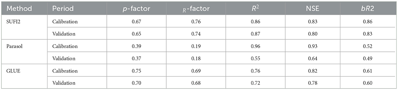
Table 3. Evaluation of model performance in simulated and observed flow during the (2011–2013) calibrating and 2 years (2014–2015) validation periods.
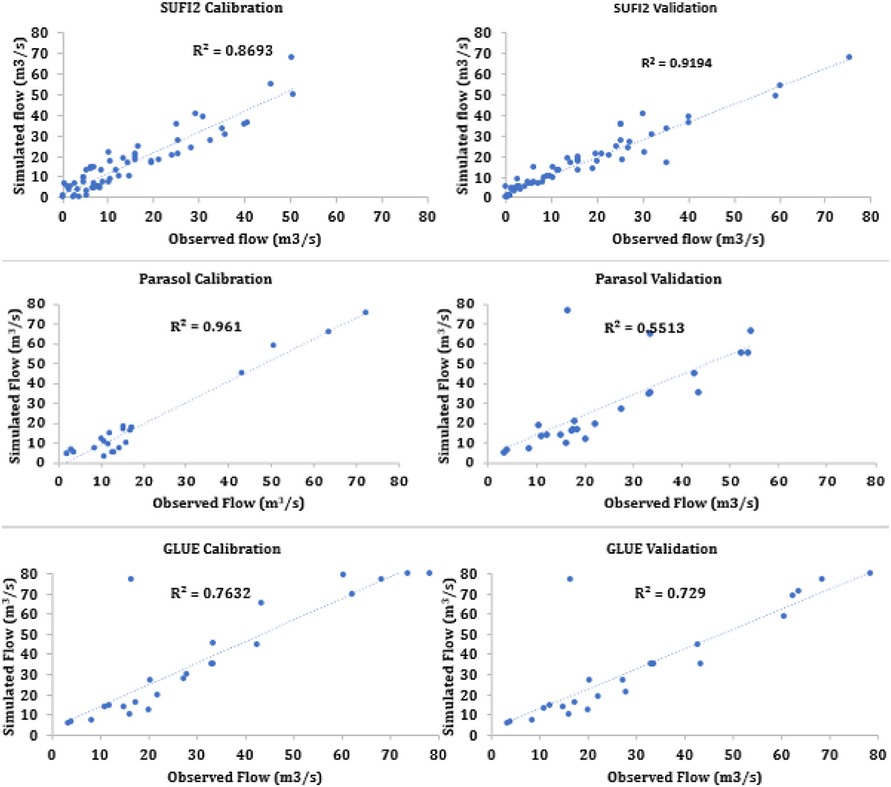
Figure 4. Scatterplot between the best simulation and observation with 95 confidence intervals.
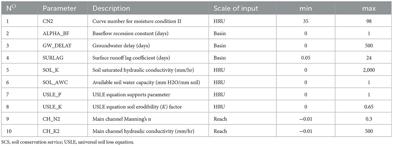
Table 4. Calibration-related variables and their absolute values.
As can be seen from Table 3, in calibration, the p-factor and r-factor yielded by ParaSol (0.39 and 0.19) were less than those generated by SUFI2 and GLUE (0.67 and 0.75 for SUFI2 and GLUE, respectively). Also, the NSE and R2 in ParaSol (0.93 and 0.96) were higher than those yielded by SUFI2 (0.83 and 0.86) and GLUE (0.82 and 0.76), suggesting that ParaSol had its advantage on accurately seeking the optimized parameter set compared to SUFI2 and GLUE. In addition, based on the evaluation criteria (Table 3) and according to Moriasi et al. (2007), the overall model performance can be rated as “good” in both the calibration and validation periods.
In the SWAT model, the target watershed is divided into sub-basins linked by the channel network, each sub-basin is further subdivided into several hydrological response units (HRUs) of homogeneous land-use, slope, and soil characteristics. Hydrological components, nutrients, and sediment yield are simulated at the HRU level and then aggregated for each sub-basin. The detailed model description is found in Neitsch et al. (2011). The suitability of the SWAT model to estimate hydrologic processes to land-use change in Gumara watershed was assessed by Teklay et al. (2021). In this study, the SWAT model set-up followed a similar setting in Teklay et al. (2021). Therefore, this study presented only a sum- many of the model set-up and evaluation results. The watershed area was discretized into 22 sub-basins. These sub- basins were further discretized into HRUs by setting a zero percent threshold level for land-use, slope, and soil. The Penman-Monteith method was chosen to calculate reference evapotranspiration (Gebre et al., 2015). The Soil Conservation Service Curve Number and the variable storage method were used to calculate surface runoff and flow routing, respectively. Based on the previous studies in the region and literature survey (Setegn et al., 2008; Gebremicael et al., 2013; Dile et al., 2016), ten SWAT model parameters were considered in this research. The ranges of model parameters and fitted values are shown in Table 4. The model parameters were calibrated and validated using the Sequential Uncertainty Fitting version 2 (SUFI-2) in the SWAT-Calibration and Uncertainty Procedure (SWAT-CUP) pack- age (Arnold et al., 2012), the model was calibrated using monthly streamflow data for a period of 15 years from 1990 to 2004. The calibration was performed through a “trial and error” process by manually adjusting the parameter ranges based on published literature (Arnold et al., 2012; Dile et al., 2016; Fentaw et al., 2018). After calibration, the model was validated using streamflow data from 2005 to 2015.
When examining calibration methods for water and soil modeling, numerous difficulties emerge. We emphasized addressing the more important concerns, which include:
1. Differences in theories and subjective decisions: Most algorithms used in calibration have their unique theories and require subjective decisions regarding prior parameter dispersals and objective functions. To overcome this issue, we selected objective functions that are commonly used in hydrological applications for each algorithm. As a result, this method led to various subjective processes for several algorithms. When analyzing the results, we specifically mention if any challenges arise from the theoretical framework of a particular algorithm or the selection of the function.
2. Lack of comparability due to different concepts and objective functions: Each algorithm is built on its fundamental concept and employs specific objective functions. This makes it difficult to compare them directly. To be able to address this problem, we calculated the value of each objective function for every algorithm. This allowed a reasonable accordance among the different techniques.
3. Evaluated the measurements of efficiency of computation and assessed the conceptual basis criteria to enhance the comparison process.
4. Each algorithm generates distinct outcomes. To tackle this issue, we carefully examined the results of all the algorithms for various criteria. We fully outlined these outcomes, allowing the reader to form their own conclusions in accordance with the provided information.
Moreover, we acknowledged that the outcomes of the comparison are inherently influenced by the specific applications. To resolve this concern, we separated the specific results of each algorithm application from the general ones, ensuring a more accurate evaluation.
The five important criteria were used to compare the three calibration algorithms (GLUE, ParaSol, and SUFI-2): Numerous parameters were incorporated into the calibration procedures.
Every technique produces unique estimations and levels of uncertainty for these parameters. Therefore, the initial comparison centers around the optimal estimate, minimum and maximum uncertainty ranges, and parameter correlation for each algorithm (Jahani et al., 2019). As different algorithms utilize various objective functions, the second evaluation is based on metrics such as NSE (Nash-Sutcliffe Efficiency), R2, and other objective functions. The third requires consideration of the R-factor, which represents the standard deviation of the band's mean width derived from the corresponding measured variable, and the P-factor, which indicates the percentage of data contained within the 95PPU (95% Prediction Performance Uncertainty) band of each algorithm. The fourth assessment was made as a result of theoretical principles, readability, and statistical criteria being met. The final assessment was made as a result of implementation difficulties (Figure 5).
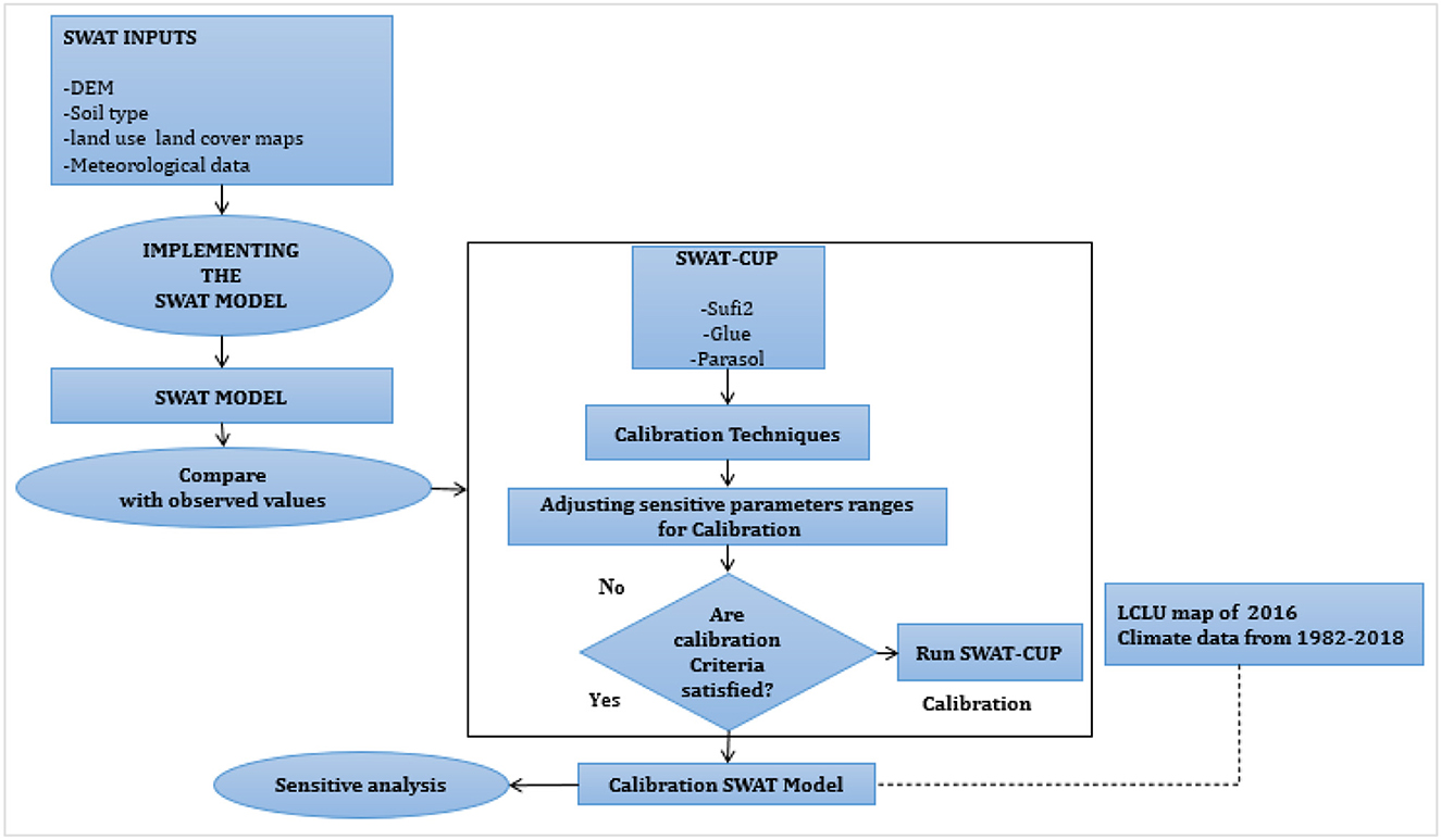
Figure 5. SWAT model calibration flowchart.
The basin area and drainage channel are both included in the basin, creating a morphometric division. It's a basin unit with naturally occurring boundaries that are characterized by similar physical characteristics, topographic patterns on the land, and climatic circumstances (Adnan et al., 2019). Basin delineation involves marking the margins of a basin on a map, typically using data from a DEM or contour maps. In SWAT modeling, the process begins with defining the basins, where the DEM serves as the input. Streams and outlet points are produced by considering the basin's slope (Sisay et al., 2017). The researcher identifies the basin's outlet locations. Additional input, such as reservoir data and designated streams, can be provided by the user. In this particular study, the area of the basin was separated into 25 smaller basins.
In Figure 6, the depicted image showcases the specified research region's allocated basin, streams, and observation locations. The subsequent step involves analyzing HRUs. The area of basin was separated into units by the HRU analysis that has topographic features, soil types, and similar land types. In this particular research, the area of basin was split into 30,70 HRUs using the soil map, and user soil data, The research area was analyzed using a map of LULC and a slope map (Figure 1). Afterward, the model was enhanced by integrating the climate database. In the final stages, the evapotranspiration, runoff, and particle outputs for each sub-basin and HRU during 35 years were calculated using the SWAT model.
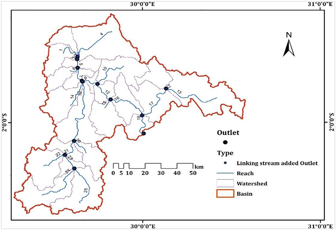
Figure 6. Basin delineation.
In this particular research, the Nile Nyabarongo River basin was assessed by using the SWAT model. The basin was divided into 25 sub-basins and 3,070 hydrologic HRUs to ensure accurate and efficient modeling. The annual average amount of rainfall in the basin was measured at 798.4 mm, with no snowfall or snowmelt. The surface runoff (Q) amounted to 81.46 mm, while the lateral discharge was measured at 105.32 mm. The deep and shallow reservoirs contributed 53 mm and 8.53 mm of groundwater discharge, correspondingly. The typical recharge for aquifers, water yield, and evapotranspiration were determined as 71.79 mm, 243.18 mm, and 559.5 mm respectively. Figure 7 presents a visual illustration of the SWAT model's productivity, focusing on runoff and evapotranspiration. The particular outcomes indicate that more than 50% of the whole precipitation is lost through evapotranspiration and runoff. Table 4 displays the average monthly values of various characteristics in the basin, such as precipitation, snowstorm, surface runoff, lateral runoff, water yield, and evapotranspiration.
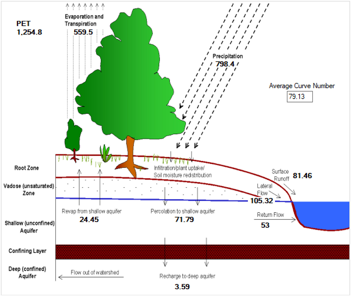
Figure 7. A pictorial illustration of the SWAT output.
The landcover land use classification in the basin consisted of five categories (illustrated in Figure 1). The majority of the basin was identified as cropland. The mean yearly rates for parameters unique to each land use type are shown in Table 5. The findings demonstrate that excessive surface runoff may occur in forestland, wetland, and agricultural land, while in the case of cropland, it remains below 15% of the water yield for the base flow. Considering that more than half of the precipitation is lost to drainage, the sediment production is similarly fairly large.
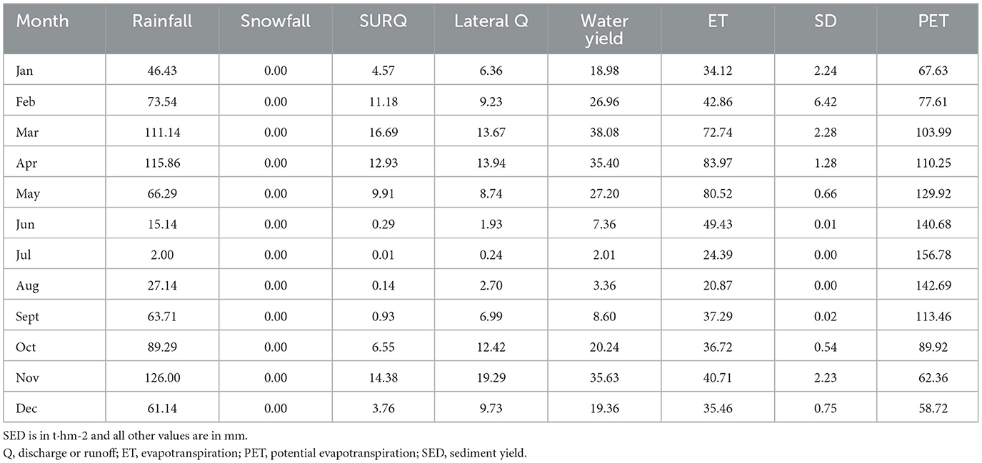
Table 5. The basin's characteristics' mean value per month.
The loss of sediment from the landscape depends on various factors. In SWAT, overestimation of sediment often occurs due to insufficient biomass production, which is particularly common in certain land use practices. Unfortunately, there is usually no measurable data can be obtained to differentiate between sediment from upland areas and sediment in streams. Streams can either contribute sediment to the overall system or act as sinks for sediment (Figure 6). The alteration of sediment within streams is influenced by physical characteristics such as channel slope, width, depth, cover, and substrate, as well as the total quantity of sediment and flow coming from upstream. Due to the evaluation of at least one HRU, the maximum sediment yield was discovered to exceed 85 thm-2 (Table 6). The collective sediment load of the entire basin was estimated to be 16.43 t-hm. Figure 8 provides a visual depiction of the sediment provides results obtained from SWAT. The highest sediment yield from upland areas is 245.02 Mg/ha, while the average yield is 16.48 Mg/ha, as indicated by the research findings.
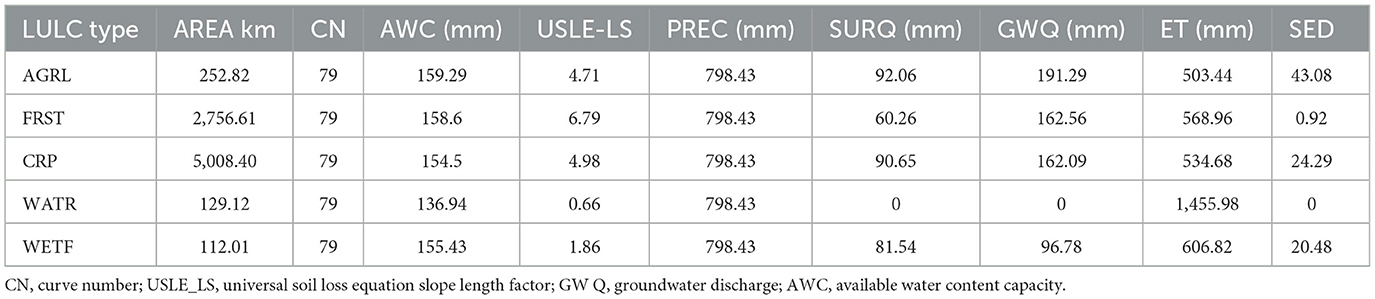
Table 6. Average annual values of the parameters for each land type.
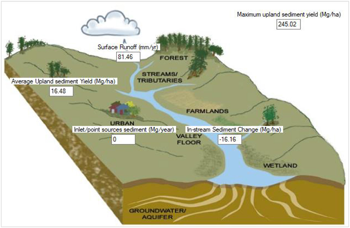
Figure 8. SWAT output for sediment yield.
Table 7 presents a summary of the calibration algorithms and their comparison. The analysis was conducted across five categories, and the outcomes are as follows:
1. In the first category, GLUE outperforms SUFI-2 and ParaSol in terms of uncertainty range. GLUE covers a larger number of intervals compared to ParaSol and SUFI-2. SUFI-2 takes the second position in this category.
2. For the second category, ParaSol, which relies on a global optimization method, achieves the highest value for its objective function, NSE. From the table values, it is evident that SUFI-2 and GLUE have similar values and hold a comparable position.
3. In the third category, ParaSol performs poorly compared in addition to the further two-algorithm approach due to its narrow prediction uncertainty bands. In accordance with the available data, SUFI-2 surpasses GLUE in this category.
4. When it comes to the fourth category, SUFI-2 and GLUE account for all unpredictability origins, whereas ParaSol solely focuses on parameter uncertainty and disregards other uncertainties. Conceptually, SUFI-2 is preferred over ParaSol and GLUE as it yields more efficient outcomes.
5. In the fifth category, GLUE stands out as the best option since it is the simplest among the three algorithms.
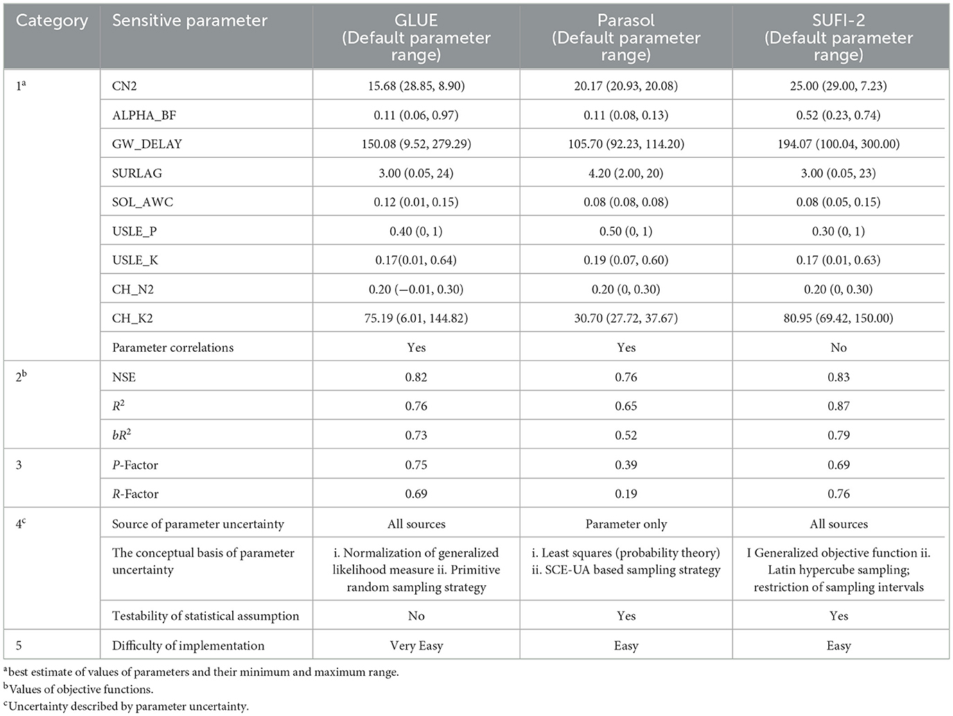
Table 7. Comparing calibration methods using the provided criteria in Section 4.5.
After analyzing and comparing the findings in Section 5.3, it might be described that the outcomes SUFI-2 and GLUE have a lot in prevalent. Nevertheless, when examining the 95PPU plot (Figure 9), it becomes evident that SUFI-2 outperforms GLUE in terms of accuracy and handling uncertainty. SUFI-2 also demonstrates efficiency by utilizing lowered quantities of variables compared to GLUE, which relies on a large number of simulations. GLUE's existence of the fundamental criticism calculation due to its random sampling approach. Consequently, for this research, SUFI-2 was selected as the superior algorithm, and only SUFI-2 was employed for further validation and calibration of sediment yield.
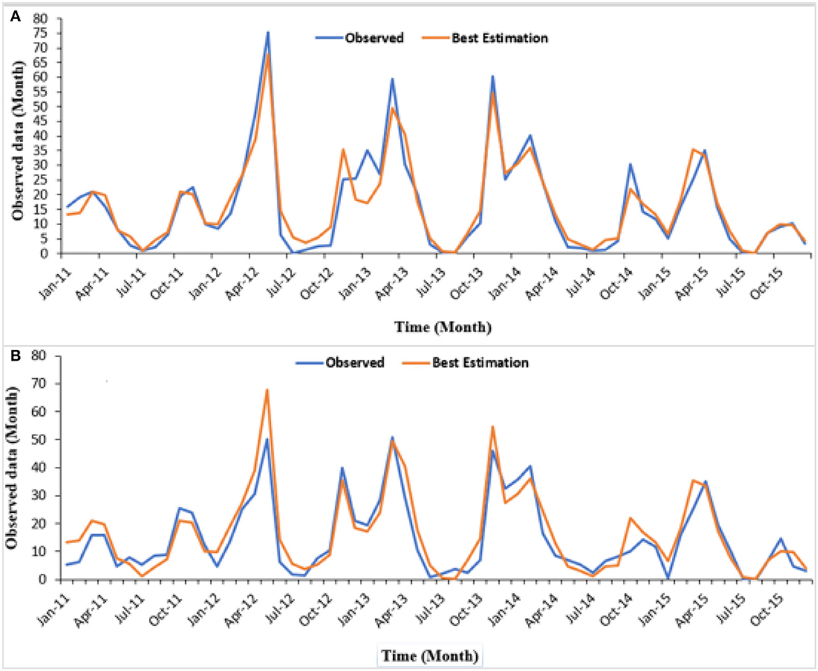
Figure 9. Plot of estimated and observed values after calibration using (A) GLUE, (B) SUFI-2.
These differences in parameters can be justified by the changing land surface characteristics and the topographic features of the basin. The justification for differences in parameter values can be based on several aspects noting that each basin has its unique characteristics, such as time stability, topography, soil types, land cover, and climate, which result in variations in parameter values (Kelleher et al., 2015). Furthermore, considering experience and similar work in a basin, model is calibrated for different periods and the optimal model parameter values vary over these periods, this can have several causes (Merz et al., 2011; Westra et al., 2014). Changes in the catchment may have occurred that are not incorporated in the model. Processes like climate change (Peel and Blöschl, 2011) land use change (Nanda et al., 2016) and the construction of hydrological structures like dikes (Weigel et al., 2014) can affect the hydrological system and, therefore, affect the optimal model parameter values in different calibration periods if these processes are not incorporated in the model (Merz et al., 2011) determined the time stability of optimal parameter values for six 5-year periods between 1976 and 2006 in 273 Austrian catchments and found considerable variation in optimal snow and soil moisture parameter values. However, it's important to note that regional variations may exist due to differences in climate, geology, and hydrological processes.
To estimate the amount of flow from the catchment, sensitivity analysis was done to identify the parameters most relevant in affecting the streamflow simulation (Mind'je et al., 2021). Table 4 shows the detected parameters to be important in regulating the streamflow generation for all the simulations. In the study area, number 1 was “very sensitive,” from number 2 to 5 “sensitive” while number 6 to 10 was slightly sensitive. From the SWAT initial estimations, these parameters were related to runoff and adjusted to suit the model simulations with the observed flow data. In SWAT, these parameters are usually used to calibrate the base flow, which was confirmed by Harka et al. (2020). The entire simulation was performed daily from 2005 to 2007 was a warm-up period. Data from the period 2011–2013 was used for calibration, and the data period 2014–2015 was used for validation. Generally, as confirmed by the previous literature related to model validations (Chaibou Begou et al., 2016), there are no rules of thumb for selecting the proportion of calibration and validation datasets depending on the available amount of data. Due to limited observed data similar to this study, Mourad et al. (2005) suggested using the larger portion of the data for calibration and the smaller portion of the data for validation. Chaibou Begou et al. (2016) also recommended using the split-sample approach, by splitting the discharge measurement data into two datasets: two-thirds for calibration and the other one for validation. Therefore, the available observed data in the study area were split from the period 2011–2013 was used for calibration, and the data period 2014–2015 was used for validation (Figure 10). The statistical performance of the model was considered satisfactory (Moriasi et al., 2007) with 0.87 R2 and 0.87 of the NSE for calibration, and 0.80 of R2 and 0.87 of NSE for validation.
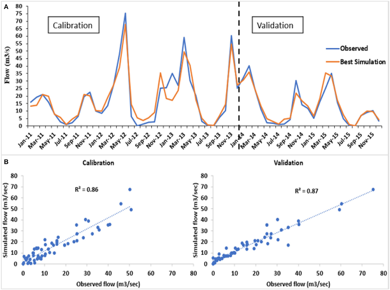
Figure 10. (A) Monthly calibration and validation for 2011–2013 and 2014–2015, (B) Comparison of observed and simulated monthly flow calibration and validation.
Throughout this evaluation, we calibrated the model using specific parameters listed in Table 3. We identified four factors that have a substantial influence on modeling the current basin in accordance with the assessment measures of the implemented model. These factors are recommended for a month-to-month time cycle. They include the effective channel hydraulic conductivity (CH K2), Manning's n value for the main channel (CH N2), surface runoff lag time (SURLAG), and the universal soil-loss equation (USLE) with a particular focus on the support parameter (USLE P).
To carry out the validation and calibration, we divided the data into different periods. The period from 2005 to 2007 served as a warm-up period. We used data from 2007 to 2011 for calibration and data from 2011 to 2015 for validation (Figure 11). The outcomes of the validation and calibration procedures are illustrated in Figure 10, respectively.
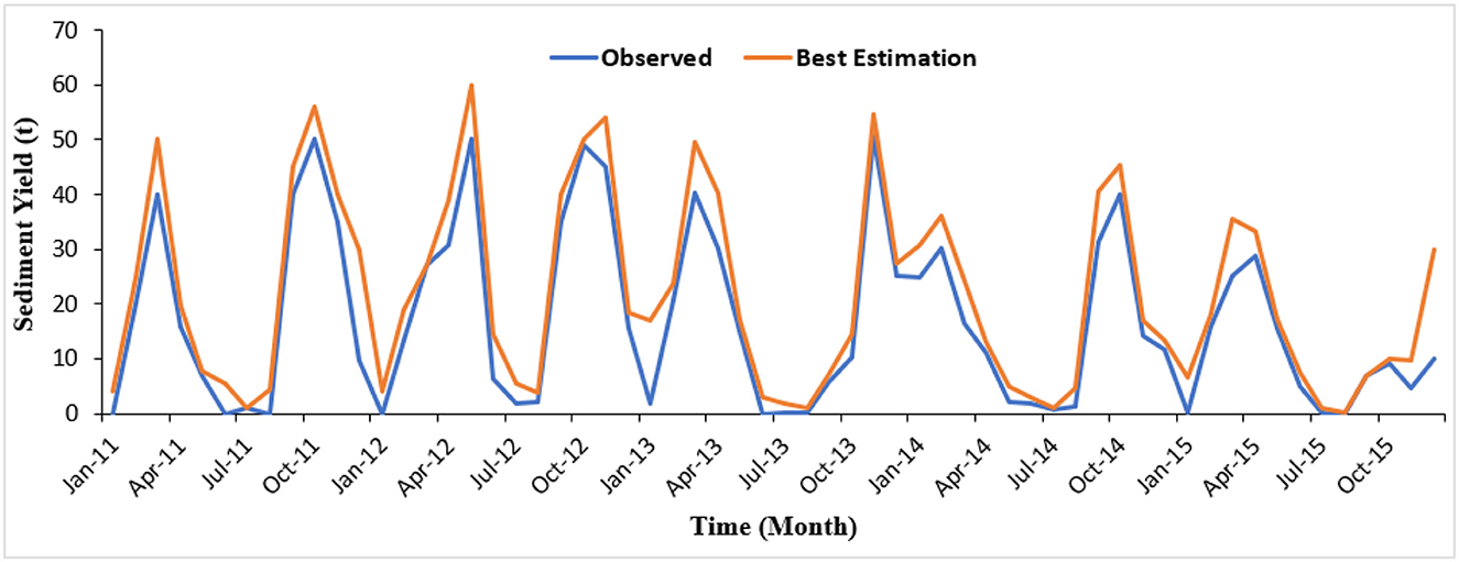
Figure 11. The graph shows sediment yield numbers, both calculated and measured (mm).
Figure 7 depicts a graph depicting the expected and measured discharge values, while Figure 8 shows a graph depicting the estimated and measured sediment data values after calibration. The measured outputs in sub-basin 19 were evaluated at the same outlet location.
Table 7 provides the values of the coefficients of appraisal for different objective functions in the research basin, specifically for the monthly yield of sediment simulation. The table presents the assessment coefficients for various objective functions and their corresponding month-to-month sediment yield simulations. The P-factor, indicating the proportion of observations within the 95% prediction uncertainty (95PPU), is 0.77, while the R-factor stands at 0.81. These results suggest that SUFI-2 produced a smaller percentage of the observed sediment yield. Moreover, moderate indicators such as R2 = 0.87, NSE = 0.83, PBIAS = 1.4 × 10² (representing percent bias), and RSR = 0.41 (the ratio of observation standard deviation) indicate a satisfactory level of fit for the model, falling within acceptable assessment ranges (Table 8). The findings demonstrate the model of SWAT effectively replicates the hydrological landscapes of the Nile Nyabarongo basin, making it an important tool for next hydrological studies around the basin.

Table 8. Objective function values.
The performance of the SWAT model was assessed using two qualitative statistics recommended by Moriasi et al. (2007): Nash-Sutcliffe Efficiency (NSE) value and Percent Bias (PBIAS). The results of the model calibration showed that the simulated mean monthly streamflow in the calibration period agrees well with the observed records, with NSE and PBIAS values of 0.89 and 10.7%, respectively. For the validation period, the NSE and PBIAS model performance of the SWAT model was 0.85 and 8.7%, respectively. These findings are in agreement with previous studies in the region (Setegn et al., 2008; Gebremicael et al., 2013; Dile et al., 2016). This research investigated three different methods for analyzing uncertainties in a hydrological model called SWAT. The study focused on the Nile Nyabarongo basin and evaluated the model's performance in simulating streamflow. The results indicated that the SWAT model produced acceptable results, with NSE and R2 values of 0.81 and 0.83 for calibration, and 0.87 and 0.87 for validation. The sensitivity analysis of four key parameters showed that ParaSol, SUFI2, and GLUE were suitable for assessing parameter sensitivity in the study area. Specifically, CH N2, SURLAG, USLE, and USLE P were found to have significant impacts on peak flow, average flow, and low flow, respectively. However, other parameters like ALPHA_BF, CH_K2, and SOL_AWC had less influence in this particular region. While ParaSol was effective in identifying the optimal parameter set, it had limitations in deriving appropriate parameter and prediction uncertainty ranges due to its narrower 95% confidence interval (CI), poor P-factor, and R-factor. On the other hand, SUFI2 and GLUE performed better in predicting parameter uncertainty, with SUFI2 outperforming GLUE in terms of the P-factor and R-factor. Overall, the SUFI2 method proved to be more favorable than the other two methods for analyzing parameter uncertainty in the SWAT model within the Nile Nyabarongo basin. It is important to note that these findings should be validated through further applications in different areas to ensure their generalizability. Additionally, apart from parameter uncertainty, it is crucial to consider the uncertainty associated with model structure and input data for a comprehensive understanding of the model's behavior. The results of this study have practical implications for water management decision-making in the region. Future research should focus on determining appropriate cultivation patterns and mitigating their negative environmental impacts to address the water crisis in the basin effectively.
Furthermore, this study demonstrates the value of using simultaneous calibration algorithms for improving SWAT model performance in data-scarce regions such as the Nyabarongo River basin. The simultaneous calibration of multiple parameters led to improved hydrological-considered processes simulation providing the best model performance. The findings of the calibrated SWAT model provide a significant tool for water resources planning in the study area and highlights the benefits of simultaneous calibration algorithms for developing robust hydrological models in data-limited regions. Further work should focus on incorporating additional observed data and testing the calibrated model for simulations of climate and land use change scenarios.
The original contributions presented in the study are included in the article/supplementary material, further inquiries can be directed to the corresponding author.
AG: Conceptualization, Visualization, Writing—original draft, Writing—review and editing. CX: Funding acquisition, Investigation, Supervision, Conceptualization, Resources, Writing—original draft. AK: Resources, Software, Supervision, Conceptualization, Data curation, Writing—review and editing. TL: Methodology, Software, Supervision, Conceptualization, Visualization, Writing—review and editing. HB: Conceptualization, Investigation, Visualization, Resources, Writing—review and editing. JU: Conceptualization, Visualization, Project administration, Writing—review and editing. AU: Conceptualization, Visualization, Resources, Writing—review and editing. UD: Conceptualization, Visualization, Validation, Writing—review and editing.
The author(s) declare financial support was received for the research, authorship, and/or publication of this article. This study was made possible with the support of various funding sources including the Key Program of National Natural Science Foundation of China (42230708) and the Strategic Priority Research Program of the Chinese Academy of Sciences, Pan-Third Pole Environment Study for a Green Silk Road (Grant No. XDA20060303), and this research was also jointly supported by the K. C. Wong Education Foundation (GJTD-2020-14), the National Natural Science Foundation of China (32071655), and the Chinese Academy of Sciences President's International Fellowship Initiative (PIFI, Grant No. 2017VCA0002).
The authors desire to acknowledge the support provided by the Chinese Academy of Science (UCAS) in funding this research. They also extend their gratitude to the Rwanda Meteorology Agency and the Ministry of Natural Resources (MINIRENA) in the Sector of Water Resources within the Rwanda Water and Forestry Authority (RWFA) for supplying the necessary daily meteorological data and daily discharge extents of the Nile Nyabarongo River.
The authors declare that the research was conducted in the absence of any commercial or financial relationships that could be construed as a potential conflict of interest.
All claims expressed in this article are solely those of the authors and do not necessarily represent those of their affiliated organizations, or those of the publisher, the editors and the reviewers. Any product that may be evaluated in this article, or claim that may be made by its manufacturer, is not guaranteed or endorsed by the publisher.
Abbaspour, K. (2014). Calibration and Uncertainty Programs—A User Manual. Paper Presented at the Proceedings of the SWAT-CUP Workshop. Dübendorf: Swiss Federal Institute of Aquatic Science and Technology (Eawag).
Abbaspour, K. C., Johnson, C. A., and Van Genuchten, M. T. (2004). Estimating uncertain flow and transport parameters using a sequential uncertainty fitting procedure. Vadose Zone J. 3, 1340–1352. doi: 10.2136/vzj2004.1340
Adams, E. A. (2017). Thirsty slums in African cities: household water insecurity in urban informal settlements of Lilongwe, Malawi. Int. J. Water Res. Develop. 4, 1–19.
Adnan, M. S. G., Dewan, A., Zannat, K. E., and Abdullah, A. Y. M. (2019). The use of watershed geomorphic data in flash flood susceptibility zoning: a case study of the Karnaphuli and Sangu river basins of Bangladesh. Nat. Hazards 99, 425–448. doi: 10.1007/s11069-019-03749-3
Akbari, F., Shourian, M., and Moridi, A. (2022). Assessment of the climate change impacts on the watershed-scale optimal crop pattern using a surface-groundwater interaction hydro-agronomic model. Agri. Water Manag. 265, 107508. doi: 10.1016/j.agwat.2022.107508
Akoko, G., Le, T. H., Gomi, T., and Kato, T. J. W. (2021). A review of SWAT model application in Africa. Water 13, 1313. doi: 10.3390/w13091313
Alawamy, J. S., Balasundram, S. K., Mohd Hanif, A. H., and Boon Sung, C. T. (2020). Detecting and analyzing land use and land cover changes in the region of Al-Jabal Al-Akhdar, Libya using time-series landsat data from 1985 to 2017. Sustainability 11, 4490. doi: 10.3390/su12114490
Arnold, J. G., Moriasi, D. N., Gassman, P. W., Abbaspour, K. C., White, M. J., Srinivasan, R., et al. (2012). SWAT: model use, calibration, and validation. Transact. ASABE 55, 1491–1508. doi: 10.13031/2013.42256
Bagheri, M., Schembari, F., Pourmousavian, N., Zare-Hoseini, H., Hasko, D., Staszewski, R. B., et al. (2020). A mismatch calibration technique for SAR ADCs based on deterministic self-calibration and stochastic quantization. IEEE Transact. Circ. Sys. I Regular Pap. 67, 2883–2896. doi: 10.1109/TCSI.2020.2985816
Baird, A. J., and Low, R. G. J. H. P. (2022). The water table: its conceptual basis, its measurement and its usefulness as a hydrological variable. Hydrol. Proc. 36, e14622. doi: 10.1002/hyp.14622
Beven, K., and Smith, P. (2015). Concepts of information content and likelihood in parameter calibration for hydrological simulation models. J. Hydrol. Engin. 20, A4014010. doi: 10.1061/(ASCE)HE.1943-5584.0000991
Boughton, W. (1989). A review of the USDA SCS curve number method. Soil Res. 27, 511–523. doi: 10.1071/SR9890511
Chaibou Begou, J., Jomaa, S., Benabdallah, S., Bazie, P., Afouda, A., Rode, M., et al. (2016). Multi-site validation of the SWAT model on the Bani catchment: model performance and predictive uncertainty. Water 8, 178. doi: 10.3390/w8050178
Devia, G. K., Ganasri, B. P., and Dwarakish, G. S. (2015). A review on hydrological models. Aquatic Proc. 4, 1001–1007. doi: 10.1016/j.aqpro.2015.02.126
Dile, Y. T., Daggupati, P., George, C., Srinivasan, R., and Arnold, J. (2016). Introducing a new open source GIS user interface for the SWAT model. Environ. Modell. Software 85, 129–138. doi: 10.1016/j.envsoft.2016.08.004
Fard, M. D., and Sarjoughian, H. S. (2021). A RESTful framework design for componentizing the water evaluation and planning (WEAP) system. Simulat. Modell. Pract. Theory 106, 102199. doi: 10.1016/j.simpat.2020.102199
Fentaw, F., Hailu, D., Nigussie, A., and Melesse, A. M. (2018). Climate change impact on the hydrology of Tekeze Basin, Ethiopia: projection of rainfall-runoff for future water resources planning. Water Conserv. Sci. Engin. 3, 267–278. doi: 10.1007/s41101-018-0057-3
Fuka, D. R., Collick, A. S., Kleinman, P. J., Auerbach, D. A., Harmel, R. D., Easton, Z. M., et al. (2016). Improving the spatial representation of soil properties and hydrology using topographically derived initialization processes in the SWAT model. Hydrol. Process. 30, 4633–4643. doi: 10.1002/hyp.10899
Gatwaza, O. C. (2016). Impact of urbanization on the hydrological cycle of migina catchment, Rwanda. Open Access Lib. J. 3, 1. doi: 10.4236/oalib.1102830
Gebre, S. L., Ludwig, F. J. J. o. C., and Forecasting, W. (2015). Hydrological response to climate change of the upper blue Nile River Basin: based on IPCC fifth assessment report (AR5). J. Climatol. Weather Forecast. 3, 1–15.
Gebremicael, T., Mohamed, Y., Betrie, G., Van der Zaag, P., and Teferi, E. J. (2013). Trend analysis of runoff and sediment fluxes in the Upper Blue Nile basin: a combined analysis of statistical tests, physically-based models and landuse maps. J. Hydrol. 482, 57–68. doi: 10.1016/j.jhydrol.2012.12.023
Giordan, D., Cignetti, M., Godone, D., Peruccacci, S., Raso, E., Pepe, G., et al. (2020). A new procedure for an effective management of geo-hydrological risks across the “Sentiero Verde-Azzurro” trail, Cinque Terre National Park, Liguria (North-Western Italy). Sustainability 12, 561. doi: 10.3390/su12020561
Harka, A. E., Roba, N. T., and Kassa, A. K. (2020). Modelling rainfall runoff for identification of suitable water harvesting sites in Dawe River watershed, Wabe Shebelle River basin, Ethiopia. J. Water Land Develop. 47, 186–195.
Heuvelmans, G., Garcia-Qujano, J. F., Muys, B., Feyen, J., and Coppin, P. (2005). Modelling the water balance with SWAT as part of the land use impact evaluation in a life cycle study of CO2 emission reduction scenarios. Hydrol. Proc. Int. J. 19, 729–748. doi: 10.1002/hyp.5620
Irankunda, E., Török, Z., Mereu?ă, A., Gasore, J., Kalisa, E., Akimpaye, B., et al. (2022). The comparison between in-situ monitored data and modelled results of nitrogen dioxide (NO2): case-study, road networks of Kigali city, Rwanda. Heliyon 8, 12. doi: 10.1016/j.heliyon.2022.e12390
Jahani, B., Mohammadi, B. J. T., and Climatology, A. (2019). A comparison between the application of empirical and ANN methods for estimation of daily global solar radiation in Iran. Theoret. Appl. Climatol. 137, 1257–1269. doi: 10.1007/s00704-018-2666-3
Kabirigi, M., Mugambi, S., Musana, B. S., Ngoga, G. T., Muhutu, J. C., Rutebuka, J., et al. (2017). Estimation of Soil Erosion Risk, Its Valuation, and Economic Implications for Agricultural Production in Western Part of Rwanda.
Kan, G., He, X., Ding, L., Li, J., Liang, K., Hong, Y., et al. (2017). A heterogeneous computing accelerated SCE-UA global optimization method using OpenMP, OpenCL, CUDA, and OpenACC. Water Sci. Technol. 76, 1640–1651. doi: 10.2166/wst.2017.322
Karamage, F., Zhang, C., Ndayisaba, F., Shao, H., Kayiranga, A., Fang, X., et al. (2016). Extent of cropland and related soil erosion risk in Rwanda. Sustainability 8, 609. doi: 10.3390/su8070609
Kelleher, C., Wagener, T., and McGlynn, B. (2015). Model-based analysis of the influence of catchment properties on hydrologic partitioning across five mountain headwater subcatchments. Water Resour. Res, 51, 4109–4136. doi: 10.1002/2014WR016147
Khaddor, I., Achab, M., Ben Jbara, A., and Hafidi Alaoui, A. (2019). Estimation of peak discharge in a poorly gauged catchment based on a specified hyetograph model and geomorphological parameters: Case study for the 23–24 October 2008 flood, KALAYA basin, Tangier, Morocco. Hydrology 6, 10. doi: 10.3390/hydrology6010010
Khatun, S., Sahana, M., Jain, S. K., Jain, N. J., and Environment. (2018). Simulation of surface runoff using semi distributed hydrological model for a part of Satluj Basin: parameterization and global sensitivity analysis using SWAT CUP. Model. Earth Sys. Environ. 4, 1111–1124. doi: 10.1007/s40808-018-0474-5
Kumar, N., Singh, S. K., Srivastava, P. K., and Narsimlu, B. (2017). SWAT Model calibration and uncertainty analysis for streamflow prediction of the Tons River Basin, India, using Sequential Uncertainty Fitting (SUFI-2) algorithm. Model. Earth Sys. Environ. 3, 30. doi: 10.1007/s40808-017-0306-z
Kuria, A. W., Barrios, E., Pagella, T., Muthuri, C. W., Mukuralinda, A., Sinclair, F. L., et al. (2019). Farmers' knowledge of soil quality indicators along a land degradation gradient in Rwanda. Geoderma Reg. 16, e00199. doi: 10.1016/j.geodrs.2018.e00199
Kwisanga, J. M. P. (2017). Assessing Flood Risk And Developing A Framework For A Mitigation Strategy Under Current And Future Climate Scenarios In Nyabarongo Upper Catchment, Rwanda.
Liu, R., Xu, F., Zhang, P., Yu, W., and Men, C. (2016). Identifying non-point source critical source areas based on multi-factors at a basin scale with SWAT. J. Hydrol. 533, 379–388. doi: 10.1016/j.jhydrol.2015.12.024
Ma, T., and Sb, T. (2020). Soil and water conservation activity on crop production and productivity in Ethiopia: a review paper. Soil Sci. 2, 122.
Mapes, K. L., and Pricope, N. G. (2020). Evaluating SWAT model performance for runoff, percolation, and sediment loss estimation in low-gradient watersheds of the Atlantic coastal plain. Hydrology 7, 21. doi: 10.3390/hydrology7020021
Martínez-Mena, M., Carrillo-López, E., Boix-Fayos, C., Almagro, M., Franco, N. G., Díaz-Pereira, E., et al. (2020). Long-term effectiveness of sustainable land management practices to control runoff, soil erosion, and nutrient loss and the role of rainfall intensity in Mediterranean rainfed agroecosystems. Catena 187, 104352. doi: 10.1016/j.catena.2019.104352
Mashingaidze, N., Ekesa, B., Ndayisaba, C. P., Njukwe, E., Groot, J. C., Gwazane, M., et al. (2020). Participatory exploration of the heterogeneity in household socioeconomic, food, and nutrition security status for the identification of nutrition-sensitive interventions in the rwandan highlands. Front. Sustain. Food Sys. 4, 47. doi: 10.3389/fsufs.2020.00047
Mengistu, A. G., van Rensburg, L. D., and Woyessa, Y. E. J. J. o. H. R. S. (2019). Techniques for calibration and validation of SWAT model in data scarce arid and semi-arid catchments in South Africa. J. Hydrol. Reg. Stud. 25, 100621. doi: 10.1016/j.ejrh.2019.100621
Merz, R., Parajka, J., and Blöschl, G. (2011). Time stability of catchment model parameters: implications for climate impact analyses. Water Resour. Res. 47, 2. doi: 10.1029/2010WR009505
Mind'je, R., Li, L., Kayumba, P. M., Mindje, M., Ali, S., and Umugwaneza, A. (2021). Integrated geospatial analysis and hydrological modeling for peak flow and volume simulation in Rwanda. Water 13, 2926. doi: 10.3390/w13202926
Moriasi, D. N., Arnold, J. G., Van Liew, M. W., Bingner, R. L., Harmel, R. D., Veith, T. L., et al. (2007). Model evaluation guidelines for systematic quantification of accuracy in watershed simulations. Transact. ASABE 50, 885–900. doi: 10.13031/2013.23153
Mourad, M., Bertrand-Krajewski, J. L., and Chebbo, G. (2005). Calibration and validation of multiple regression models for stormwater quality prediction: data partitioning, effect of dataset size and characteristics. Water Sci. Technol. 52, 45–52. doi: 10.2166/wst.2005.0060
Nanda, R., Chow, L. Q., Dees, E. C., Berger, R., Gupta, S., Geva, R., et al. (2016). Pembrolizumab in patients with advanced triple-negative breast cancer: phase Ib KEYNOTE-012 study. J. Clin. Oncol. 34, 2460. doi: 10.1200/JCO.2015.64.8931
Neitsch, S. L., Arnold, J. G., Kiniry, J. R., and Williams, J. R. (2011). Soil and Water Assessment Tool Theoretical Documentation Version 2009.
Nsengimana, V., Weihler, S., and Kaplin, B. A. (2017). Perceptions of local people on the use of Nyabarongo River wetland and its conservation in Rwanda. Soc. Nat. Res. 30, 3–15. doi: 10.1080/08941920.2016.1209605
Nsengiyumva, J. B., and Valentino, R. (2020). Predicting landslide susceptibility and risks using GIS-based machine learning simulations, case of upper Nyabarongo catchment. Geom. Nat. Hazards Risk 11, 1250–1277. doi: 10.1080/19475705.2020.1785555
Ogden, F. L., and Saghafian, B. (1997). Green and Ampt infiltration with redistribution. J. Irrig. Drain. Engin. 123, 386–393. doi: 10.1061/(ASCE)0733-9437(1997)123:5(386)
Omara, T., Nteziyaremye, P., Akaganyira, S., Opio, D. W., Karanja, L. N., Nyangena, D. M., et al. (2020). Physicochemical quality of water and health risks associated with consumption of African lung fish (Protopterus annectens) from Nyabarongo and Nyabugogo rivers, Rwanda. BMC Res. Notes 13, 66. doi: 10.1186/s13104-020-4939-z
Peel, M. C., and Blöschl, G. (2011). Hydrological modelling in a changing world. Prog. Phys. Geography 35, 249–261. doi: 10.1177/0309133311402550
Pradhan, P., Tingsanchali, T., and Shrestha, S. (2020). Evaluation of soil and water assessment tool and artificial neural network models for hydrologic simulation in different climatic regions of Asia. Sci. Total Environ. 701, 134308. doi: 10.1016/j.scitotenv.2019.134308
Radcliffe, D. E., and Mukundan, R. (2017). PRISM vs. CFSR precipitation data effects on calibration and validation of SWAT models. JAWRA J. Am. Water Res. Assoc. 53, 89–100. doi: 10.1111/1752-1688.12484
Rahvareh, M., Motamedvaziri, B., Moghaddamnia, A., and Moridi, A. (2023). Modeling runoff management strategies under climate change scenarios using hydrological simulation in the Zarrineh River Basin, Iran. J. Water Clim. Change. 4, 511. doi: 10.2166/wcc.2023.511
Rutebuka, J., Kagabo, D. M., and Verdoodt, A. (2019). Farmers' diagnosis of current soil erosion status and control within two contrasting agro-ecological zones of Rwanda. Agric. Ecosyst. Environ. 278, 81–95. doi: 10.1016/j.agee.2019.03.016
Setegn, S. G., Srinivasan, R., and Dargahi, B. J. T. O. H. J. (2008). Hydrological modelling in the Lake Tana Basin, Ethiopia using SWAT model. Open Hydrol. J. 2, 1. doi: 10.2174/1874378100802010049
Shivhare, N., Dikshit, P. K. S., and Dwivedi, S. B. (2018). A comparison of swat model calibration techniques for hydrological modeling in the ganga river watershed. Engineering 4, 643–652. doi: 10.1016/j.eng.2018.08.012
Singh, A., Imtiyaz, M., Isaac, R., and Denis, D. J. A. W. M. (2012). Comparison of soil and water assessment tool (SWAT) and multilayer perceptron (MLP) artificial neural network for predicting sediment yield in the Nagwa agricultural watershed in Jharkhand, India. Agricult. Water Manag. 104, 113–120. doi: 10.1016/j.agwat.2011.12.005
Sisay, E., Halefom, A., Khare, D., Singh, L., and Worku, T. (2017). Hydrological modelling of ungauged urban watershed using SWAT model. Model. Earth Sys. Environ. 3, 693–702. doi: 10.1007/s40808-017-0328-6
Tejaswini, V., and Sathian, K. (2018). Calibration and validation of swat model for Kunthipuzha basin using SUFI-2 algorithm. Int. J. Curr. Microbiol. Appl. Sci. 7, 2162–2172. doi: 10.20546/ijcmas.2018.701.260
Teklay, A., Dile, Y. T., Asfaw, D. H., Bayabil, H. K., and Sisay, K. (2021). Impacts of climate and land use change on hydrological response in Gumara Watershed, Ethiopia. Ecohydrol. Hydrobiol. 21, 315–332. doi: 10.1016/j.ecohyd.2020.12.001
Uwacu, R. A., Habanabakize, E., Adamowski, J., and Schwinghamer, T. D. (2021). Using radical terraces for erosion control and water quality improvement in Rwanda: a case study in Sebeya catchment. Environ. Develop. 4, 100649. doi: 10.1016/j.envdev.2021.100649
Wasko, C., and Nathan, R. J. (2019). Influence of changes in rainfall and soil moisture on trends in flooding. J. Hydrol. 575, 432–441. doi: 10.1016/j.jhydrol.2019.05.054
Weigel, F. K., Hazen, B. T., Cegielski, C. G., and Hall, D. J. (2014). Diffusion of innovations and the theory of planned behavior in information systems research: a metaanalysis. Commun. Assoc. Inform. Sys. 34, 31. doi: 10.17705/1CAIS.03431
Westra, S., Fowler, H. J., Evans, J. P., Alexander, L. V., Berg, P., Johnson, F., et al. (2014). Future changes to the intensity and frequency of short-duration extreme rainfall. Rev. Geophy. 52, 522–555. doi: 10.1002/2014RG000464
Wolka, K., Mulder, J., and Biazin, B. (2018). Effects of soil and water conservation techniques on crop yield, runoff and soil loss in Sub-Saharan Africa: a review. Agricult. Water Manag. 207, 67–79. doi: 10.1016/j.agwat.2018.05.016
Wu, H., and Chen, B. (2015). Evaluating uncertainty estimates in distributed hydrological modeling for the Wenjing River watershed in China by GLUE, SUFI-2, and ParaSol methods. Ecol. Eng. 76, 110–121. doi: 10.1016/j.ecoleng.2014.05.014
Wu, H., Chen, B., Snelgrove, K., and Lye, L. (2019). Quantification of uncertainty propagation effects during statistical downscaling of precipitation and temperature to hydrological modeling. J. Environ. Inform. 34, 139–148.
Yamashita, S., Watanabe, R., and Shimatani, Y. (2015). Smart adaptation to flooding in urban areas Proc. Engin. 118, 1096–1103. doi: 10.1016/j.proeng.2015.08.449
Yuan, L., Sinshaw, T., and Forshay, K. J. J. G. (2020). Review of watershed-scale water quality and non-point source pollution models. Geosciences 10, 25. doi: 10.3390/geosciences10010025
Zhang, D., Chen, X., Yao, H., and James, A. (2016). Moving SWAT model calibration and uncertainty analysis to an enterprise Hadoop-based cloud. Environ. Modell. Software 84, 140–148. doi: 10.1016/j.envsoft.2016.06.024
Zhang, X., Srinivasan, R., and Bosch, D. J. (2009). Calibration and uncertainty analysis of the SWAT model using genetic algorithms and bayesian model averaging. J. Hydrol. 374, 307–317. doi: 10.1016/j.jhydrol.2009.06.023
Zhao, F., Wu, Y., Qiu, L., Sun, Y., Sun, L., Li, Q., et al. (2018). Parameter uncertainty analysis of the SWAT model in a mountain-loess transitional watershed on the Chinese Loess Plateau. Water 10, 690. doi: 10.3390/w10060690
Keywords: calibration algorithm, hydrology, SWAT, Nyabarongo River, Rwanda
Citation: Gasirabo A, Xi C, Kurban A, Liu T, Baligira HR, Umuhoza J, Umugwaneza A and Dufatanye Edovia U (2023) SWAT model calibration for hydrological modeling using concurrent methods, a case of the Nile Nyabarongo River basin in Rwanda. Front. Water 5:1268593. doi: 10.3389/frwa.2023.1268593
Received: 28 July 2023; Accepted: 11 September 2023;
Published: 06 October 2023.
Edited by:
Reza Kerachian, University of Tehran, IranReviewed by:
Ali Moridi, Shahid Beheshti University, IranCopyright © 2023 Gasirabo, Xi, Kurban, Liu, Baligira, Umuhoza, Umugwaneza and Dufatanye Edovia. This is an open-access article distributed under the terms of the Creative Commons Attribution License (CC BY). The use, distribution or reproduction in other forums is permitted, provided the original author(s) and the copyright owner(s) are credited and that the original publication in this journal is cited, in accordance with accepted academic practice. No use, distribution or reproduction is permitted which does not comply with these terms.
*Correspondence: Chen Xi, Y2hlbnhpQG1zLnhqYi5hYy5jbg==
Disclaimer: All claims expressed in this article are solely those of the authors and do not necessarily represent those of their affiliated organizations, or those of the publisher, the editors and the reviewers. Any product that may be evaluated in this article or claim that may be made by its manufacturer is not guaranteed or endorsed by the publisher.
Research integrity at Frontiers
Learn more about the work of our research integrity team to safeguard the quality of each article we publish.