 Grigorios Kyritsakas
 Joby Boxall
 Vanessa Speight
- Department of Civil and Structural Engineering, Sheffield Water Centre, The University of Sheffield, Sheffield, United Kingdom
A novel data-driven model for the prediction of bacteriological presence, in the form of total cell counts, in treated water exiting drinking water treatment plants is presented. The model was developed and validated using a year of hourly online flow cytometer data from an operational drinking water treatment plant. Various machine learning methods are compared (random forest, support vector machines, k-Nearest Neighbors, Feed-forward Artificial Neural Network, Long Short Term Memory and RusBoost) and different variables selection approaches are used to improve the model's accuracy. Results indicate that the model could accurately predict total cell counts 12 h ahead for both regression and classification-based forecasts—NSE = 0.96 for the best regression model, using the K-Nearest Neighbors algorithm, and Accuracy = 89.33% for the best classification model, using the combined random forest, K-neighbors and RusBoost algorithms. This forecasting horizon is sufficient to enable proactive operational interventions to improve the treatment processes, thereby helping to ensure safe drinking water.
1. Introduction
Drinking water treatment plants (DWTPs) are complicated systems tasked with processing raw water to produce high-quality drinking water that complies with the regulatory standards. The treatment process consists of different steps from pre-treatment to disinfection that are monitored with sensors connected to the supervisory control and data acquisition (SCADA) system. The SCADA systems offer a real-time check of the flow entering and exiting the various treatment stages, the quality of the water exiting each treatment stage, the quality of the treated water exiting the DWTP, and the condition and the operational status (on/off) of the electromechanical equipment (pumps, valves, chemical mixers etc.) and the water level of any tanks. Drinking water quality is monitored through SCADA via the sensor detection of the key water quality indicator variables including pH, turbidity, and disinfectant residual with a frequency between 5 to 15 min. Moreover, samples are collected with a daily frequency at the DWTPs outlet to measure key water quality parameters such as coliform bacteria, heterotrophic plate counts, chlorine and turbidity (DWI, 2020).
DWTP staff use the collected data to adapt the treatment processes to address changes in the flow or the quality of the water entering the plant. These interventions in the treatment process, such as changing chemical doses and adjusting flow rates, are mostly reactive and are made once issues have been identified (Tomperi et al., 2014). Often, the reaction time is insufficient to prevent water quality deterioration, particularly for source water with rapidly changing conditions such as rivers with significant anthropogenic impacts (Jayaweera et al., 2019). Previous research to model water treatment has been based on mathematical models and empirical formulas describing the complex systems of chemical and biological reactions; however, this has proven to be difficult due to the complexity and interactions of the physical, chemical and biological processes involved (Ghandehari et al., 2011; Wang and Xiang, 2019).
1.1. Application of machine learning for DWTP management
Given the large data availability in DWTPs, data-driven models that apply machine learning (ML) methodologies are gaining in popularity as an alternative to mathematical and empirical modeling, providing accurate and proactive solutions in many cases. Their main advantage in comparison to the other modeling types is their ability to use as inputs different types of data that are coming from different sources and have different structure and frequency. Moreover, data-driven models are capable to understand non-linear relationships in the data and uncover hidden relationships between different water quality parameters that measure the quality of the water in the different DWTPs' processes. Thus, data-driven models have been utilized for the optimization of processes in DWTPs (Zhang et al., 2013; Park et al., 2015; Jayaweera et al., 2019), predicting future deterioration events (Fu et al., 2017; Mohammed et al., 2017), and improving the overall performance of the DWTP (Abba et al., 2020). In these works, the authors utilized the data that the DWTPs' SCADA systems already collected to improve the treatment management. A number of recent studies that applied ML methodologies in DWTPs are presented in a review paper by Li et al. (2021). In this paper, the authors presented ML based research works that were successful applied in different DWTP's process stages for improving the coagulation dosing and the membranes optimization and design, controlling the membranes fouling and accurately predicting water quality events. The authors strongly believe that ML based models have the potential to provide further knowledge regarding the treatment processes and fully support decision making. However, they argue that more work is required on interpretable methods that will better simulate the water treatment problems. Moreover, for them, future work should focus on detection methods that provide useful data for analysis of complex contaminants in the treatment processes and on ML decision-making systems that will revolutionize the DWTPs automation control system.
Prior research rarely considers the bacteriological presence in the water, those that exist focus either on the prediction or control of bacteria in the water source or the optimization of the disinfection process (Haas, 2004). There is a gap in the applications of ML techniques to provide information regarding bacteriological presence in the treated water. This paper aims to fill this gap with a ML based methodology that predicts bacteriological presence in the water exiting DWTPs.
1.2. Cell counting data
With the absence of regulations in online sensor monitoring to quantify the presence of bacteria in the DWTPs, bacteriological monitoring of the drinking water relies on manual collection of water quality samples from the DWTP outlet to measure coliform bacteria and heterotrophic plate counts (HPC) (DWQR, 2019; DWI, 2020). Laboratory analysis for these bacteriological indicator variables is time consuming, with the results not available for at least one day after the sample was collected. Therefore, potential bacteriological failures will only be identified once the water has passed in the drinking water distribution system (DWDS). In addition, as this process cannot be automated, the results are not incorporated directly into the SCADA system for use in system control. At present, sensors for the bacteriological real time monitoring are under development with the main technologies being presented in a UK Water Innovation Research report (Boxall et al., 2020).
Given that HPC is a century-old approach that typically captures <1% of the bacteria in the drinking water, flow cytometry (FCM) is becoming an alternative method to measure bacteriological presence (Hammes et al., 2008). FCM is capable of counting the total number of bacterial cells (TCCs) in the bulk water thereby providing a better understanding of the overall bacteriological concentration than HPC (Van Nevel et al., 2016, 2017). Moreover, an online FCM has been developed that can produce results with high frequency in an automated process (Besmer et al., 2016; 2014). Potential application of this technology in the DWTP could transform the manual sampling for bacteriological monitoring into an automated process that could be controlled and checked from the SCADA system. Furthermore, online FCM could generate a large data set that could be further analyzed in data-driven models to understand the bacteriological content of the treated water. However, the application of online FCM technology has some challenges to overcome such as the high cost of the FCM hardware, the integration in the existing automation systems and the requirement of an efficient data standardization methodology that guaranties high quality microbial data (Besmer et al., 2014).
This paper explores the potential application of FCM with ML modeling by developing a data-driven forecasting model for the prediction of the bacteriological presence, expressed as TCCs, in the treated water (DWTP outlet). The model is designed for both regression and classification forecasting and its ability is tested in a large operational DWTP, located in the north of the UK, that serves a population of circa 600,000 people, for a year of hourly operational data. Both predictive approaches were used as the regression one could indicate the bacterial cells change over a certain period and the classification one could set an alarm when the cell numbers surpass a certain threshold. The data-driven model used different ML methods with the aim to compare and select those methods with better predictive performance. Moreover, different input variables selection methodologies (feature selection) were examined with the aim to improve the predictive performance, reduce the computational cost, and improve interpretability. Finally, a combination between the best model outputs (selected based on their performance metrics) was examined for a potential increase in the model's accuracy. The aim was to develop a novel tool that could predict elevated bacteriological presence in DWTPs outlets with a sufficient lead time to allow for adjustments to improve the overall treatment efficiency of the DWTP.
2. Materials and methodology
2.1. Site description and selected data
The case study DWTP serves part of a large city, located in the north of the UK, as well the surrounding area in the east of this city, and has a maximum capacity of 364,000 m3/day. The DWTP treats raw water from two different nearby lakes via a pre-treatment stage followed by coagulation (alum), flocculation, filtration (double-staged rapid gravity filters), and disinfection with chlorine. For the chlorination process, the filtered water is dosed with hypochlorite before reaching the disinfection contact tank. The hydraulic retention time (HRT) of the treatment process is estimated to be roughly 8 h. Once past the chlorine contact tank, the treated water is stored in the treated water service reservoir (SR) for a further 11 h (SR_RT). Finally, the treated water reaches the distribution networks via 2 pump stations (1 main +1 backup). A flow schematic of the DWTP that includes the flow and water quality variables sensor locations is presented in Figure 1.
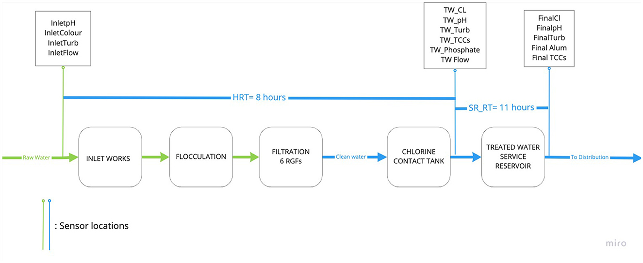
Figure 1. Case study DWTP flow schematic including flow and water quality variables measurement sensor location (see table 1 for short-name clarification).
The SCADA system at this site collects water quality and flow data from the DWTP inlet, DWTP outlet, and from the outlet of each treatment process tank with 5 min frequency. The measured water quality indicator variables at this site include turbidity and pH at the inlet (InletTurb, InletpH), the outlet (FinalTurb, FinalpH) and the treatment stages (TW_Turb, TW_pH), color at the inlet (Inletcolour), chlorine (Cl2) in the disinfection contact tank outlet (TW_Cl) and at the outlet (FinalCl). Increased bacteriological presence has been measured in the water exiting the plant on several occasions in recent years so the water utility installed 2 online FCMs to measure TCCs, with a frequency of one measurement every 1 to 2 h, at the exit of the disinfection tank and at the outlet of the treated water service reservoir. In addition, discrete water quality samples are collected, between a daily and a weekly basis, at the SR outlet and analyzed for different water quality indicator variables. However, these parameters are not included in this work because the aim is to develop a fully automated model that uses data that are automatically provided by the DWTP SCADA system. The flow and water quality indicator variables used in this study are presented in the following table (Table 1).
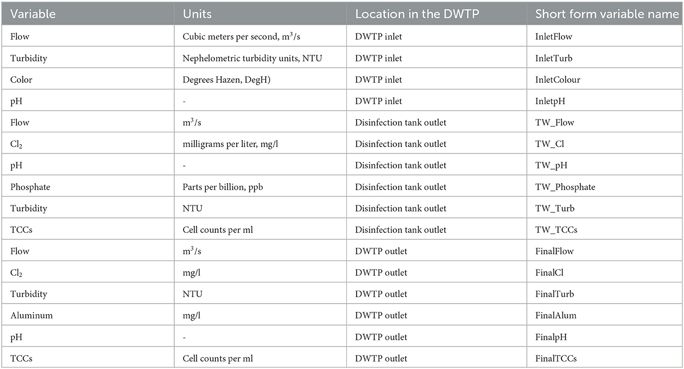
Table 1. Summary of the DWTP variables used in this work.
TCCs monitoring by online FCM started September 1st, 2020, and thus, the study period for this investigation is between the 31st of August 2020 (to include antecedent conditions) through September 1st 2021 which was the installation period for the two online FCMs in this particular DWTP. Descriptive statistics for the variables during the study period are presented in Table 2. Due to the difference in the measurement frequency between the DWTP's flow and water quality indicator variables and the online FCM TCCs, all data were transformed to hourly time step data (from 5 min data) using the mean of each variable in the hourly time bin. However, as the FCM data had an hourly or bihourly frequency, the missing TCC data were filled using the cubic spline interpolation, with the descriptive statistics of the actual and the interpolated TCC data presented in Supplementary Table S1.
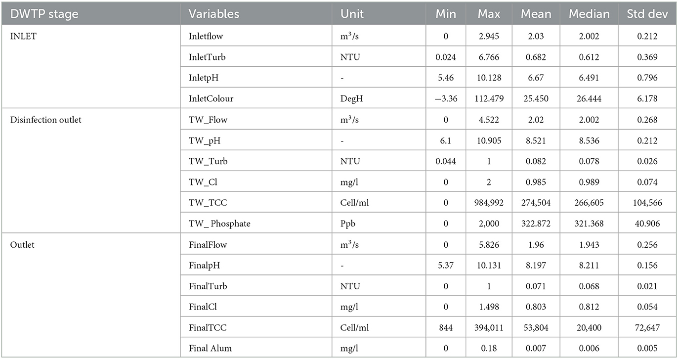
Table 2. Descriptive statistics for DWTP variables used in this study.
The hourly time series dataset required reorganization to capture the time lags in the DWTP. The overall retention time in the DWTP was estimated to be approximately 19 h [HRT (8) + SR_RT (11)]. So, for example, water that entered the plant at 00:00 h would exit the disinfection tank at 08:00 h on that same day and reach the distribution network at 19:00 h, still on that same day. The TCCs predictive horizon was set to be 12 h ahead (sufficient time for operational interventions), which means that for the forecasting model, the TCC measurement from the water exiting the DWTP at 19:00 h (and associated upstream samples) will be used to predict the TCCs at the DWTP outlet on the following day at 07:00 h. The dataset was reorganized as presented in Figure 2.

Figure 2. A schematic of the reorganization of the dataset to fill the time lags between the various treatment stages and forecasting horizon of 12 h.
2.2. Data preparation and model input variables
The regression forecasting approach requires the model to predict the actual TCC values in the DWTP outlet 12 h into the future. For this approach, the dataset was split into inputs and outputs, where inputs were the data in the inlet, the disinfection tank outlet and the plant outlet and the outputs the TCCs in the outlet 12 h ahead (Figure 3). For the classification forecasting approach, the output TCCs were categorized in 4 different classes, based on the water utility's risk criteria (Table 3). The distribution of data is highly imbalanced, as Table 3 indicates, with more than 45% of the samples belonging in minimum risk class, while <30% of the samples belonging in the risk classes (classes 2 and 3).
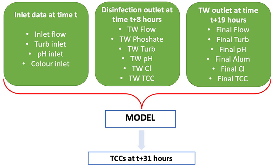
Figure 3. Simplified diagram of the first group of inputs and outputs of the TCCs predictive model.
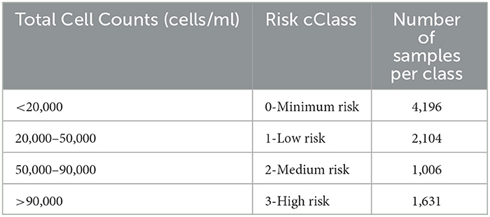
Table 3. Risk ranking classes for water exiting the DWTP.
Figure 3 shows the initial group of variables (16 variables) used in the TCCs predictive model for both the classification and the regression approaches. However, as past work in this field has shown, including daily peaks or averages of various variables and increasing the input sliding window that consequently increases the total number of input variables, could also increase the model's accuracy (Meyers et al., 2017). Thus, in this investigation, two other variable groups were tested. More specifically, in the second group of variables, the daily peak and average inlet flow, outlet flow, inlet turbidity, treated water TCCs, and final TCCs 2 days before the output TCCs were added to the initial input group resulting in a total number of 26 input variables. Finally, in the third group of variables, a 5-h sliding window was selected, in addition to the second group of variables, resulting in a total number of 106 input variables (16 initial, 5 averages and 5 peaks and 5 x 16 variables for the previous 5 time-lags). The 3 different input sets are presented in Table 4.
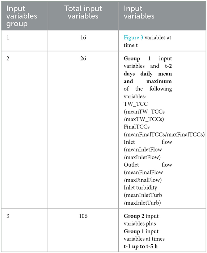
Table 4. Input variables groups for the predictive model.
The dataset was divided into training set and testing set using the k-fold cross validation approach (Kohavi, 1995). In our case, the dataset was split into 20 folds to avoid a small training set, given that the available dataset is not a large one and covers just a 12-month period. However, the model was tested randomly in only 4 of the of the overall 20 folds, the 5th, the 8th, the 12th and the 15th folds. All 4 folds captured data from the different seasons of the year study period. The k-fold methodology was implemented using MATLAB version 2022b and the training / testing ratio for each fold was 85%−15%.
Once the training and test datasets were created and before training the model, the input and output data (for the regression approach only) were standardized (scaled to have mean 0 and standard deviation 1).
2.3. Machine learning methods
The predictive model was developed in MATLAB version 2022b using the Statistics and Machine Learning and the Deep Learning toolboxes. The ML methods used in the model were as follows:
2.3.1. Random forest
RF is an ensemble of weak independent decision trees ML method that uses a randomly selected number of variables from the initial input variables group to make its splitting decision at each node (Breiman, 2001). RF was used for both the classification and the regression forecast. In classification, the final class decision is made using one vote per tree, while in regression the final output value is the average value of the weak trees. In this work, the number of the weak trees was set equal to 1,000, the number of the randomly selected variables was set equal to the square of the total number of the input variables, and the minimum tree leaf per tree was set equal to 2.
2.3.2. Support vector machines
SVM is a supervised ML method that constructs a high dimensional linear decision space (hyperplane) to map the low-dimensional but non-linear inputs (Cortes and Vapnik, 1995). SVM uses a kernel function to transform the features in the hyperplane. The kernel function selected for this work was the Gaussian kernel and SVM was used for both the regression and the classification forecast.
2.3.3. K-nearest neighbors
KNN is a simple non-parametric instant-based ML method that produces outputs based on the outputs of the K closest training examples (Hastie et al., 2008). KNN was used for both classification and regression forecasts in this work, setting the number of neighbors k equal to 5 and calculating the distance between each new point and the training samples using the Euclidean distance. KNN produces its prediction outputs by voting among the k neighbors for the classification forecast and by averaging the values of the k neighbors in the regression forecast.
2.3.4. Feed-forward ANN
The ANN algorithm (Bishop, 2006) was used for the regression approach only. ANNs consist of an input layer, hidden layer(s), and an output layer and the connection between these layers is made through different transfer functions. In this work, one hidden layer with a size equal to 10 units was selected using the Bayesian hyperparameter tuning process, and the Bayesian regularization backpropagation was used as a transfer training function to update the weights and the bias values.
2.3.5. Long short-term memory
The LSTM belongs in the deep learning (DL) methodologies, an advanced sub-field of ML algorithm (Hochreiter and Schmidhuber, 1997). LSTM are a type of recurrent neural network (RNN) designed for sequence prediction as they introduce memory blocks connected via layers. Each layer consists of three gates, the input and the output gates as well as the forget gate that removes all the non-required information. LSTM was used for both classification and regression in this work. LSTM hyperparameters were set using a Bayesian optimization that indicated an LSTM network consisting of 1 hidden layer with 50 units and initial learning rate equal to 0.01.
2.3.6. RusBoost boosting trees
The RB algorithm belongs in the family of the gradient boosting trees ML methods (Seiffert et al., 2008). In gradient boosting, in contrast to RF, each new generated tree learns from the previous weak tree by using weights. RB is a classification only method. In addition to the gradient boosting, it also removes random training samples that belong in the majority class(es) to create more balanced training sets and thus tackle the class imbalance problem. In this work, the number weak trees was set equal to 1,000, the maximum number of splits per tree was set equal to the number of the training samples, and the learning rate was set equal to 0.1.
2.4. Performance metrics
The predictive model regression accuracy was evaluated using the root mean squared error (RMSE), the Scatter Index (SI), the Nash-Sutcliffe Efficiency (NSE) and the Kling-Gupta Efficiency (KGE) performance metrics. RMSE penalizes the large predictive errors, has the same units as the forecasted variable (cells/ml in our model) and have a range from 0 to infinity with values closer to 0 indicating higher accuracy (Bryant et al., 2016). SI is a normalized version of the RMSE error reported as a percentage or as values between 0 and 1 (Bryant et al., 2016). NSE is an improved version of the correlation coefficient that is commonly used in the hydrological modeling (Knoben et al., 2019). NSE's range is between -∞ and 1, with NSE<0 indicating a worse model accuracy than the mean of the observed data, NSE = 0 indicating a model with the same accuracy prediction as the mean of the observed data and NSE = 1 indicating the perfect predictive model. Finally, KGE is recently used as an alternative to NSE for hydraulic and hydrological modeling calibration and evaluation (Knoben et al., 2019). KGE has the same range and same indications as NSE. The metrics are expressed as follows:
where n = number of samples, Oi = the ith observed value, Õ = the observations mean, σO = the standard deviation of the observations, Yi = the ith predicted value, = the predictions mean, σY = the standard deviation of the predictions and CC the Pearson correlation between observations and predictions. Additional performance metrics that show the general model ability (PI) or compare similar ML methods performance when different sets of input variables are introduced (AICc) are presented in the Supplementary material.
In classification, 4 metrics were used to evaluate the model, the overall accuracy, the macro-recall, the macro-precision, the macro-F1 score and the recall of the high-risk class. Accuracy is the percentage of the accurate predictions over the total number of testing sample as given from the following equation:
Macro-recall, macro-precision, and macro-F1 score are the simple average of the recall, precision and F1 score over the 4 classes, respectively. The mathematical expressions of recall, precision and F1-score are as follows:
where TP refers to the true positives of class, TN to the true negatives of a class, and FP to the false positives. Recall per class calculates the percentage of the accurately predicted events in this class, precision per class gives the proportion of the accurately predicted events of a class over total predicted events of this class and F1-score is a formula that examines the relationship between precision and recall (Ahmed et al., 2019). The macro-average of these metrics will give an overall efficiency of the predictive model. Finally, the recall of the high-risk class was examined separately, as it is important to know how accurately the model identifies bacteriological activity that could potentially harm the consumer.
2.5. Feature selection
The aim of the feature selection is to reduce the dimensionality of the initial dataset by selecting a subset of more important input variables that could achieve similar or even more accurate predictive results than the initial model with less computational time for training and testing. In addition, feature selection methods could identify input variables that do not offer any contribution in the prediction ability of the model. In general, there are 3 types of feature selection algorithms, the Filter type, the Wrapper type, and the Embedded type. Filter type algorithms aim to identify correlations between the input variables and the target output and rank the variables based on this correlation. Wrapper type algorithms consider the selection as an optimization problem with certain criteria and aim to find the optimal input variable set that satisfies these criteria. Embedded type algorithms learn the importance of the input variables as part of the machine learning training process. Decision tree algorithms, such as RF and RusBoost, include an embedded feature selection process as part of their training. In this work, two filter and one embedded feature selection algorithm were selected as the aim was to identify the most related input variables to the output target. The three different feature selection methods that were used in this work are as follows:
2.5.1. RF predictors' importance (RFPI)—Embedded algorithm
RF is an interpretable method that in addition to the prediction that produces, it provides estimates over the influence of each unique input variable in the final prediction. In this research, the RFI was used for the selection of the input variables that had higher predictor importance value than 0.7 for the regression and higher than 1.4 for the classification.
2.5.2. Minimum redundancy maximum relevance (MRMR)—Filter algorithm
MRMR algorithm aims to find an optimal set of variables that have minimum correlation with each other but as a set have the optimum relevance with the predictive variable (Zhao et al., 2019). The MRMR algorithm, initially, selects the best input variable as the one that has the highest f-score with the output variable. The second variable is selected as the one with highest maximum output relevance minimum input variables redundancy score. This process continues for all the remaining variables. Once the process is finalized, the variables with the highest score are identified.
2.5.3. Neighborhood component feature selection (NCFS)—Filter algorithm
This approach uses the nearest neighbor decision rule to generate weighting importance for each different input variable by maximizing the leave-one-out accuracy (Yang et al., 2012). A random weight is given at each vector at the beginning of the process. The weights are then updated through an optimization with regularization process which aims to find the optimal weights that minimize the objective function which measures the average leave-one-out loss. At the end the process, the final weighting score given to each variable indicates its importance. In this work, the stochastic gradient decent was used as an objective function and the regularization parameter was selected through an optimization process.
2.6. Ensemble (combined) tests
The aim of combining tests was to investigate if the ensemble approach improves the TCC model performance. Two different approaches were used in this work, the average model and the weighted average model. The regression average model is the simple average of the predictive outputs of the best regression tests while the classification average approach produces its classification from the classification outputs of the best tests by vote. In case of a tie, the classification average model selects the higher class. In the weighted average models, a weight is assigned to each unique test based on its predictive performance. Therefore, the difference between the average and the weighted average model is that, in the former, each test contributes equally to the ensemble model output while in the latter, each test contribution is based on its predictive ability.
3. Results
3.1. Regression results
3.1.1. Initial analysis
A summary of the results of the different modeling tests is presented in Table 5 (additional metrics in Supplementary Table S2), which shows the average performance metrics of the tests in the 4 different folds. It is notable that all the predictive model tests had high NSE and KGE values (minimum NSE = 0.78 and KGE = 0.88) indicating that the predictive model is capable of capturing the behavior and patterns of interest.

Table 5. Summary of the regression model's performance metrics (in bold the best performing tests).
RF appears to be the best performing ML method, with the best results for each group of input variables (tests R1, R6, R14). Moreover, RF captured a minimum of 93% of the variance (NSE = 0.93) when the minimum number of inputs were used (test R1). KNN was ranked second, SVM third, ANN forth and LSTM was the worst performing model. The results indicate that the predictive model performs better when the 2nd group of input variables is used for the training as all the ML methods had their best results when this group of variables was used. The performance decrease when the 3rd group of variables is used indicates that adding more variables could sometimes lead to overfitting, i.e., learning patterns from time-lagged variables could confuse the model predictions. However, the overfitting did not affect all the ML methods equally, with the ANN having a drop in RMSE performance of almost 30% and SI performance of 25%. Moreover, the average RMSE average (21,768 cells/ml) is an indication that the model is weak in predicting rare and extreme values. However, this value is almost 4 times below the TCCs standard deviation.
3.1.2. Regression feature selection
In this analysis step, the 2nd group of input variables was used as input for the feature selection as it was with this group of variables that gave the best model outputs. In the RFPI approach, the importance of each variable was equal to the average of its importance in each one of the 4 different training folds for the R6 test. The simple average of the scores and weights over the 4 different training folds was also used for the MRMR and NCFS algorithms, respectively. The results of the feature selection algorithms application are presented in Table 6 (for the importance score per variable see Supplementary material). The number of important variables was 7 for the RFPI, 4 for the MRMR, and 9 for the NCFS. The predictive model was tested again using the input variables suggested by these feature selection algorithms and the 3 best ML methods (RF, KNN and SVM) from the initial analysis. Overall, 9 more tests were implemented (3 groups of variables x 3 ML methods) and the results are presented in Table 7 (additional performance metrics in Supplementary Table S5).
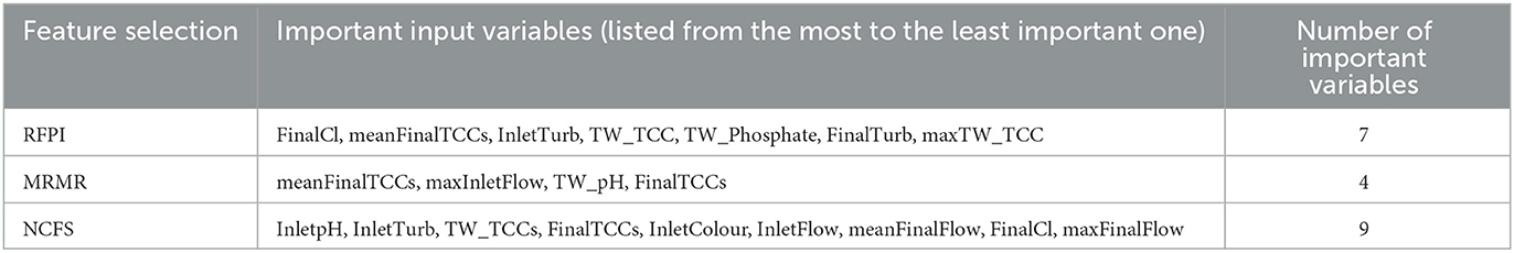
Table 6. The most important input variables for RFPI, MRMR and NCFS feature selection approaches.
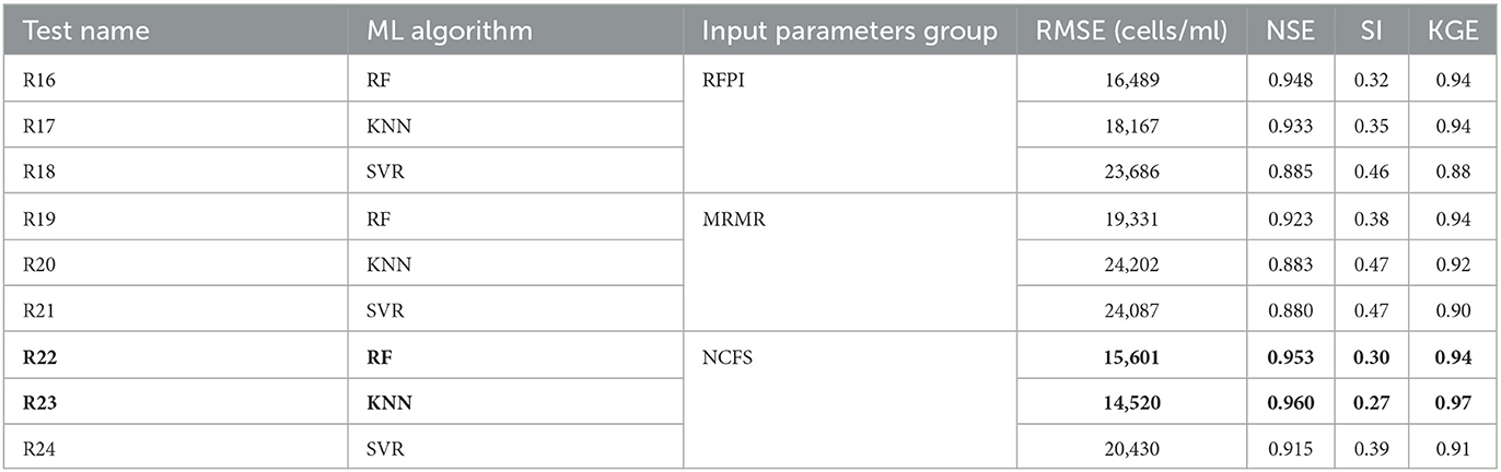
Table 7. Regression predictive model performance metrics using the variables indicated by the feature selection algorithms (in bold the best performing tests).
NCFS is the best out of the three feature selection algorithms, with all the ML methods having their best performance when the input variables suggested by the NFCS were used. Moreover, the results of the R22 and R23 tests indicate that the predictive model's performance was improved beyond its best performance in the initial analysis (test R6). RFPI's input selection produced worse predictions than both the best RF test and best SVR test (R10). However, when the RFPI's inputs were used, KNN had better performance than the initial analysis (R17 and R9, respectively).
Tests R19, R20, R21 showed that all ML methods had worse results than in the initial analysis, however these MRMR results were better than tests where the group 1 input variables were used (R1, R4, R5). This finding indicates the importance of the daily average and the daily maximum of some key variables, such as flow and TCCs, for better prediction results. KNN's RMSE performance was improved by more than 3,500 cells/ml, its NSE and KGE performance by 2% and 3% respectively, and its SI performance by 8% when NCFS input variables were used, a result that made R23 the overall best predictive test output. As R22 is slightly better performing test in comparison to R6, it was this test that was selected together with the R23 test for the ensemble approach.
3.1.3. Ensemble (combined) analysis
For the ensemble analysis the results from test R22 and R23 (overall best performing models) were combined using the average and the weighted average of their predictive outputs. In the average ensemble (AM), both tests contributed equally to the final output (predicted TCCs) as this was the average of both tests. In the weighted average ensemble (WAM), the final output used a 60% to 40% weighted average of the R23 and R22 tests, respectively based on the better predictive performance of the R23 compared to R22. The results of the two ensemble approaches are presented in Table 8.
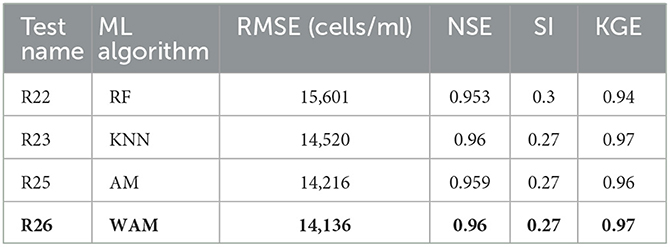
Table 8. Performance metrics of the two regression ensemble approaches and the best two single tests (in bold the best performing tests).
Both the AE and WAE had better performance than the R22 test and, as expected, R26 performed better than R25. Both R25 and R26 had better RMSE performance than the best single test (R23) indicating that the ensemble approach is more capable in capturing the unexpected or extreme values. The MAE performance of the combined approaches (R25 and R26) lies between the two single tests (R22 and R23), which is to be expected given that MAE is the average error over the testing dataset. However, we could consider R26, that uses the WAE approach, the best approach as it explains 97% of the variance (KGE = 0.97) but also its RMSE output is better than R23 by almost 400 cells/mlA comparison plot of the predicted time-series outputs of the best two single tests and the two ensemble approaches is presented in Figure 4 for a period of elevated cell data that was investigated in this work (for further graphs check the Supplementary material).

Figure 4. Plot of the observed vs. the predictive TCCs time-series produced by tests R22, R23, R25, and R26.
3.2. Classification results
3.2.1. Initial analysis
The initial classification results are presented in Table 9. The results show trends similar to the regression forecast. Specifically, as was seen for the regression approach, the 2nd group of input variables was the one that produced the best results for each ML method and RF was, overall, the best predictive ML method. However, in the classification analysis, RB also produced good results that were close to the results produced by RF. As was the case for the regression approach, LSTM was the worst performing model indicating that this ML method is not appropriate for this type of WQ investigation and with this type of available data. SVM's performance was worse than in the regression analysis, ranked this ML method as the second worst. Finally, KNN was the third best method, having significantly better macro-precision and macro-F1 results in comparison to SVM but still significantly worse than the RF and RB ML methods.
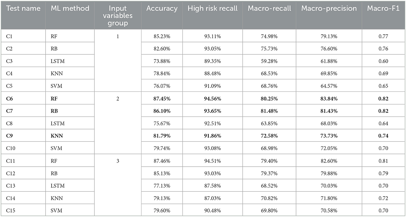
Table 9. Summary of the classification tests performance metrics (in bold the best performing tests).
3.2.2. Classification feature selection
As was the case in the regression analysis, the best three performing ML methods for the classification analysis were selected for further investigation: RF, RB, and KNN. The group of input variables that the 3 different feature selection algorithms indicated as important are given in Table 10. For this analysis as in the regression analysis, 9 different new predictive model tests were implemented, and the results are presented in Table 11.

Table 10. The most important input variables for RFPI, MRMR and NCFS feature selection algorithms for classification.
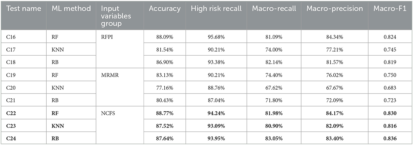
Table 11. Predictive model classification performance metrics using the variables indicated by the feature selection algorithms (in bold the best performing tests).
NCFS once again is the best input variable selection algorithm with MRMR being the worst. The performance of all three ML methods was improved when the NCFS' input variables were used as the results for the C22, C23, and C24 tests indicate. In contrast to the regression analysis results, the predictive model's performance was also improved when the RFPI input variables were used as each ML method produced better results than the initial analysis (C16, C18, and C17 better than C6, C7, and C9, respectively). NFCS feature selection improved the KNN accuracy by more than 6% (C23); however, both RF (C22) and RB (C23) had slightly better performance overall. As these three tests were the best ones, they were selected for the classification ensemble analysis.
3.2.3. Ensemble (combined) analysis
For the classification prediction model, only the average ensemble (AM) approach was used because the results of the best three single approach tests were very similar. In Table 12, a comparison of the AE with the best single tests is presented which clearly shows that the combined approach (C25) outperformed all the single tests. The only metric where C25 was worse than any of the single models was the high-risk class metric, where it was less accurate to test C24 by 0.28% and to test C22 by 0.58%. However, its higher macro-precision and macro-recall performance indicate that this model is more able to correctly predict an output in the correct class and it creates less false positives than these two single tests.
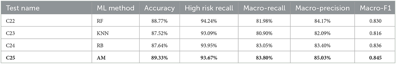
Table 12. Performance metrics of the two classification ensemble approaches and the best three single tests (in bold the best performing tests).
4. Discussion
This work aims to contribute to the discussion about implementation of data-driven modeling as a decision supporting tool for improving the performance of DWTPs. More specifically, this research, primarily, aims to propose a data-driven model that could be used as a tool to support decision making for improving the bacteriological performance of the DWTPs. The secondary aim of this work is to promote the application of online FCM, that are not yet widely in use now, as a tool that monitors bacterial presence in the treated water. Given the fact that utilities already collect this large amount of water quality time-series data, additional online FCM data could improve the present data-driven model and reduce the extreme values prediction error.
The results of the analysis present two alternative predictive approaches which offer slightly different information for water utilities about their operations. The regression predictive model could be used as a tool for understanding the variance and the distribution of the TCCs over a certain predictive period. The classification predictive model could be used as a tool that identifies when a DWTP is at a high risk of bacteriological failure, thereby requiring an intervention.
KNN was the method that resulted in the best regression predictive model in this work (R23). This model was significantly improved through the application of input variable selection techniques. This performance improvement was also seen for KNN in the classification analysis, ultimately demonstrating that KNN has great potential when the appropriate input variables are selected. In addition, KNN is simple to implement, and its results are transparent and comprehensible to decision makers and managerial stuff in water utilities. In general, KNN's main disadvantage is its computational cost as it requires time to compute the distances between the new unseen input with all the existing data, however, in this work its computational time was insignificant as the available dataset was small and not too complex.
RF is a well-known method in the water sector and has been applied in various projects (Parkhurst et al., 2005; Meyers et al., 2017; Kazemi et al., 2022). The results of this work indicate that for this dataset, it was one of the two best models for predicting TCCs at the DWTP outlet. In agreement with literature where RF was applied, it is recommended that RF be considered for WQ problems, especially if the datasets are well-distributed. RF is a simple ML method to apply, and its results could be justified and explained to decision makers due to its transparent and interpretable outputs.
The fact that LSTM was the worst performing model was not an unexpected outcome. In recent studies in the hydroinformatics field, deep learning approaches have been proven to be the models that could produce the most accurate results (Hitokoto and Sakuraba, 2018; Dairi et al., 2019; Zhou et al., 2019; Mamandipoor et al., 2020). However, the available datasets in these studies were extremely large in comparison to the available dataset in our DWTP WQ study, which is probably the reason that LSTM performed poorly. In addition, LSTM required the most computational time during the training period. This finding though does not, necessarily, indicate that LSTM is not a good method for all WQ problems. Deep learning approaches, in contrast to the traditional ML approaches, are learning directly from the examples and their multiple levels of representations over their consecutive layers (Lecun et al., 2015). Hence, a further investigation of LSTM prediction capability should be performed in case studies with larger datasets or in the later years for this case study when substantially more online TCC data becomes available.
The RB method applied in the classification approach also produced good results. In the past, it was successfully applied for the prediction of iron failures in district meter areas, which was a classification problem with unbalanced datasets (Mounce et al., 2017). In this case study, the dataset was more balanced with only the medium risk class (class 2) having fewer samples compared to the other three classes. RB increased the recall accuracy of this class which, consequently, increased the overall macro-recall accuracy. Its other advantage was its computational time that was lower than RF. However, RB's lower macro-precision performance compared to the RF indicates this ML method also produced more false positives than the RF results. This finding clearly demonstrates the importance of taking overall consideration of multiple performance metrics to decide which model is the best. Water utility decision makers should always consider the main purpose of the modeling prediction and how much compromise between true and false positives they can tolerate for their proactive water quality interventions.
This work demonstrated the importance of a feature selection process for improving the prediction capabilities of the model. NFCS improved both the regression and classification models' accuracy and, in addition, reduced the time required for collecting the data and training the model by reducing the required input variables to 9 for regression and 10 for classification. The comparison between the three different feature selection algorithms indicated that the success of each one of these algorithms is highly dependent on the type of the data-driven model. For example, MRMR algorithm identified only 4 input variables that were fully independent to each other but when the model was trained using these 4 suggested variables, it generated the worst overall prediction results. This finding may also show that, for water quality problems, using dependent input variables could be beneficial for the model accuracy.
The aim of the ensemble approach was to investigate if a combination of two or more of the best predictive tests could improve the overall model prediction accuracy for both the regression and the classification approaches. The ensemble tests are fully dependent on the accuracy of each one of the individual models and, therefore, they were not expected to produce an extreme improvement in the model prediction accuracy. Nevertheless, the ensemble approach also reduced the variance and the bias of the individual tests and, as a result, reduced the extreme values errors in regression and the false positive predictions in classification.
This paper highlights the importance of online microbiological monitoring for understanding drinking water quality. Traditional bacteriological monitoring approaches require a daily sample to measure the 4 regulated bacteriological indicator variables (DWQR, 2019). However, the traditional discrete sample monitoring cannot capture the variations of bacteria during a 24-h operational period. In addition, by measuring once per day for coliform bacteria, it can be extremely rare to find coliforms in the outlet. The online monitoring capability used in this study provided valuable information about TCC and the water quality indicator variables that influence the bacteriological presence in the water leaving the DWTP. Moreover, online monitoring can capture sudden changes in the water quality and, finally as we demonstrated in this work, can provide input for data-driven models for the prediction of potential future deterioration events.
Figure 4 and the high RMSE metric results indicate that in the regression approach, all the used ML methods struggled to predict extreme values of TCC. This inability is probably due to limitations in the available dataset, which did not capture seasonal changes in this study. There are only a few measurements in the dataset where extreme TCC values have been found, as would be expected for an operating DWTP. Therefore, the model was not able to be trained properly for prediction of extreme values. Future work, when more data is available, should focus on extreme events by using them as an extra input variable for the training period. The classification approach, on the other hand, was able to predict the water being in the high-risk class (TCCs >90,000) with an accuracy of 88% to 96%. This finding indicates that this model is able to understand the conditions when extreme TCC numbers will occur. By using this approach, utilities could benefit from a 12-h advance indication of a high bacteriological risk and act promptly.
The predictive model is a data-driven approach that does not require any hydraulic and process model for its implementation. It uses the data measurements as captured by the sensors and stored in the SCADA of the DWTP. Thus, the time that is required for its training is minimal in comparison to process-based models that require extensive inputs, hours of simulation, and high computational power. This advantage is gained because the data-driven models learn the trends and the patterns of the dataset, in contrast to process-based models that are using complex hydraulic and process equations to describe the water circulation and treatment processes. Moreover, process-based models demand many process and hydraulic empirical coefficients that require calibration, and often recalibration to match any spatial and temporal changes of the system. Finally, the data-driven model applied in this DWTP, once built, could be used in any other DWTP that has a SCADA system that contains sufficient water quality data. The process-based models, though, cannot always be directly transferred to other systems as each system has each unique process and hydraulic characteristics. Nevertheless, the scientific knowledge regarding the DWDS hydraulics and processes is a prerequisite for the implementation of the data-driven models in the DWDS to guarantee the scientific consistency of the model.
5. Conclusions
This paper has demonstrated a novel data-driven model that uses multiple machine learning methods and input variables (features) selection algorithms for the prediction of the bacteriological activity (as measured by flow cytometry total cell counts) in the water exiting a drinking water treatment plant. Models were developed using both regression and classification prediction approaches. In addition, an ensemble approach that combined the results of multiple machine learning methods was examined. Based on the results, the key findings of this research study are:
• The regression predictive model managed to capture total cell count trends and the general bacteriological behavior 12 h into the future. However, it was not able to predict the highest extreme observed peaks, probably because the available of such extreme data was limited.
• The classification model did capture the extreme events and classified the water that belongs in the high bacteriological risk class with an accuracy of up to 96%.
• Random Forest has been proven to be the best single machine learning method for both the classification model and K-Nearest Neighbor was the best single machine learning method for the regression approach.
• Neighborhood component feature selection was the best feature selection algorithms as its proposed input variables decreased the required inputs (and consequently reduced the computational time) and improved the model prediction accuracy.
• The ensemble approach, which combined the best single machine learning method results, was the best overall predictive test for both regression and classification. The regression ensemble approach combined the outputs of the best two single method tests and the classification approach the outputs of the best three single method tests.
• Long short-term memory had the worst performance out of all the machine learning methodologies. This finding was expected as deep learning approaches require much larger datasets than were available in this study. This is a constraint that will apply to many other water sector applications.
Overall, the outputs of this work advance knowledge about the operational benefits for water utilities by analyzing the water quality data that is already collected in drinking water treatment plants using data-driven predictive models. The total cell counts predictive model could be further developed as an online tool, connected to the drinking water treatment plant SCADA system. Such an online system would provide warnings to operators of a potential bacteriological risk in treated water sufficiently far ahead to adjust the treatment processes and help safeguard drinking water quality.
Data availability statement
The data analyzed in this study is subject to the following licenses/restrictions: These data belong to a water utility and cannot be shared publicly. Requests to access these datasets should be directed to Zy5reXJpdHNha2FzQHNoZWZmaWVsZC5hYy51aw==.
Author contributions
GK: methodology, model preparation, model validation, and writing—first draft. JB and VS: methodology and supervision—review and editing. All authors contributed to the article and approved the submitted version.
Funding
This work was funded by the EPSRC Centre for Doctoral Training in Engineering for the Water Sector (STREAM IDC, EP/L015412/1) and Scottish Water.
Acknowledgments
The authors gratefully acknowledge Claire Thom and Fiona Webber at Scottish Water for the data collection, their input and assistance. For the purpose of open access, the author has applied a creative commons attribution (CC BY) license to any author accepted manuscript versions arising.
Conflict of interest
The authors declare that the research was conducted in the absence of any commercial or financial relationships that could be construed as a potential conflict of interest.
Publisher's note
All claims expressed in this article are solely those of the authors and do not necessarily represent those of their affiliated organizations, or those of the publisher, the editors and the reviewers. Any product that may be evaluated in this article, or claim that may be made by its manufacturer, is not guaranteed or endorsed by the publisher.
Supplementary material
The Supplementary Material for this article can be found online at: https://www.frontiersin.org/articles/10.3389/frwa.2023.1199632/full#supplementary-material
References
Abba, S. I., Pham, Q. B., Usman, A. G., Linh, N. T. T., Aliyu, D. S., Nguyen, Q., et al. (2020). Emerging evolutionary algorithm integrated with kernel principal component analysis for modeling the performance of a water treatment plant. J. Water Pro. Engin. 33, 1081. doi: 10.1016./j.jwpe.2019.101081
Ahmed, U., Mumtaz, R., Anwar, H., Shah, A. A., and Irfan, R. (2019). Efficient water quality prediction using supervised machine learning. Water 11, 2210. doi: 10.3390./w11112210
Besmer, M. D., Epting, J., Page, R. M., Sigrist, J. A., Huggenberger, P., Hammes, F., et al. (2016). Online flow cytometry reveals microbial dynamics influenced by concurrent natural and operational events in groundwater used for drinking water treatment. Sci. Rep. 6, 1–10. doi: 10.1038./srep38462
Besmer, M. D., Weissbrodt, D. G., Kratochvil, B. E., Sigrist, J. A., Weyland, M. S., Hammes, F., et al. (2014). The feasibility of automated online flow cytometry for in-situ monitoring of microbial dynamics in aquatic ecosystems. Front. Microbiol. 5, 1–12. doi: 10.3389./fmicb.2014.00265
Bishop, C. (2006). Pattern Recognition and Machine Learning (First). Cambridge, UK: Springer US. doi: 10.1021./jo01026a014
Boxall, J., Court, E., and Speight, V. (2020). Real Time Monitoring of bacteria at Water Treatment Works and in Downstream Networks. Sheffield. Available online at: https://ukwir.org/real-time-monitoring-of-bacteria-at-water-treatment-works-and-in-downstream-networks (accessed June 21, 2023).
Bryant, M. A., Hesser, T. J., and Jensen, R. E. (2016). Evaluation Statistics Computed for the Wave Information Studies (WIS). Engineer Research and Development Centre, Coastal and Hydraulics Laboratory (Mississippi, U.S.). Available online at: https://hdl.handle.net/11681/20289
Cortes, C., and Vapnik, V. (1995). Support-vector networks. Mach. Learn. 20, 273–297. doi: 10.1023/A:1022627411411
Dairi, A., Cheng, T., Harrou, F., Sun, Y., and Leiknes, T. O. (2019). Deep learning approach for sustainable WWTP operation: a case study on data-driven influent conditions monitoring. Sustain. Cit. Soc. 50, 101670. doi: 10.1016./j.scs.2019.101670
DWI (2020). Drinking Water 2020: The Chief Inspector's Report for Drinking Water in England. London: Drinking Water Inspectorate. Available online at: https://cdn.dwi.gov.uk/wp-content/uploads/2021/07/09174358/1179-APS-England_CCS1020445030-003_Chief_Inspectors_Report_2021_Prf_52.pdf
DWQR (2019). Drinking Water Quality in Scotland 2018: Public Water Supply. Available online at: https://dwqr.scot/media/2zajlpst/dwqr-annual-report-2018-public-water-supplies.pdf
Fu, J., Lee, W. N., Coleman, C., Nowack, K., Carter, J., Huang, C. H., et al. (2017). (2017). Removal of disinfection byproduct (DBP) precursors in water by two-stage biofiltration treatment. Water Res. 3, 73. doi: 10.1016/j.watres.06073
Ghandehari, S., Montazer-Rahmati, M. M., and Asghari, M. (2011). (2011). A comparison between semi-theoretical and empirical modeling of cross-flow microfiltration using ANN. Desalination. 4, 57. doi: 10.1016/j.desal.04057
Haas, C. N. (2004). Neural networks provide superior description of Giardia lamblia inactivation by free chlorine. Water Res. 38, 3449–3457. doi: 10.1016/j.watres.05001
Hammes, F., Berney, M., Wang, Y., Vital, M., Köster, O., Egli, T., et al. (2008). Flow-cytometric total bacterial cell counts as a descriptive microbiological parameter for drinking water treatment processes. Water Res. 42, 269–277. doi: 10.1016/j.watres.07009
Hastie, T., Tibshirani, R., and Friedman, J. (2008). The Elements of Statistical Learning (Second). Stanford: Springer US. doi: 10.1007./b94608
Hitokoto, M., and Sakuraba, M. (2018). “Applicability of the deep learning flood forecast model against the flood exceeding the training events,” in Proceeding of 13th International Conference on Hydroinformatics, Palermo, Italy. Palermo.
Hochreiter, S., and Schmidhuber, J. (1997). (1997). Long short-term memory. Neural Comput. 9, 1735–1780. doi: 10.1162/neco.98.1735
Jayaweera, C. D., Othman, M. R., and Aziz, N. (2019). Improved predictive capability of coagulation process by extreme learning machine with radial basis function. J. Water Process Engin. 32, 100977. doi: 10.1016./j.jwpe.2019.100977
Kazemi, E., Kyritsakas, G., Husband, S., and Flavell, K. (2022). “Predicting iron exceedance risk in drinking water distribution systems using machine learning,” in Proceedings of the 14th International Conference on Hydroinformatics. Bucharest.
Knoben, W. J. M., Freer, J. E., and Woods, R. A. (2019). Technical note: inherent benchmark or not? Comparing Nash-Sutcliffe and Kling-Gupta efficiency scores. Hydrol. Earth Sys. Sci. 23, 4323–4331. doi: 10.5194/hess-23-4323-2019
Kohavi, R. (1995). “A study of cross-validation and bootstrap for accuracy estimation and model selection,” in Proceedings of the 14th International Joint Conference on Artificial Intelligence (pp. 1137–1143).
Lecun, Y., Bengio, Y., and Hinton, G. (2015). Deep learning. Nature 521, 436–444. doi: 10.1038/nature14539
Li, L., Rong, S., Wang, R., and Yu, S. (2021). Recent advances in artificial intelligence and machine learning for non-linear relationship analysis and process control in drinking water treatment: a review. Chem. Engin. J. 405, 6673. doi: 10.1016./j.cej.2020.126673
Mamandipoor, B., Majd, M., Sheikhalishahi, S., Modena, C., and Osmani, V. (2020). Monitoring and detecting faults in wastewater treatment plants using deep learning. Environ. Monit. Assess. 192, 1–12. doi: 10.1007/s10661-020-8064-1
Meyers, G., Kapelan, Z., and Keedwell, E. (2017). (2017). Short-term forecasting of turbidity in trunk main networks. Water Res. 124, 67–76. doi: 10.1016/j.watres.07035
Mohammed, H., Hameed, I. A., and Seidu, R. (2017). “Random forest tree for predicting fecal indicator organisms in drinking water supply,” in Proceedings of 4th International Conference on Behavioral, Economic, and Socio-Cultural Computing, BESC 2017. doi: 10.1109./BESC.2017.8256398
Mounce, S. R., Ellis, K., Edwards, J. M., Speight, V. L., Jakomis, N., Boxall, J. B., et al. (2017). Ensemble decision tree models using rusboost for estimating risk of iron failure in drinking water distribution systems. Water Res. Manag. 31, 1575–1589. doi: 10.1007/s11269-017-1595-8
Park, M., Anumol, T., and Snyder, S. A. (2015). Modeling approaches to predict removal of trace organic compounds by ozone oxidation in potable reuse applications. Environ. Sci. Water Res. Technol. 1, 699–708. doi: 10.1039/c5ew00120j
Parkhurst, D., Brenner, K., Dufour, A., and Wymer, L. (2005). Indicator bacteria at five swimming beaches—analysis using random forests. Water Res. 39, 1354–1360. doi: 10.1016/j.watres.01001
Seiffert, C., Khoshgoftaar, T. M., Van Hukse, J., and Napolitano, A. (2008). “RUSBoost: improving classification performance when training data is skewed.pdf,” in 19th International Conference on Pattern Recognition (ICPR 2008), December 8-11, 2008. Tampa, Florida, USA. doi: 10.1109/ICPR.2008.4761297
Tomperi, J., Juuso, E., Etelaniemi, M., and Leiviskä, K. (2014). Drinking water quality monitoring using trend analysis. J. Water Health 12, 230–241. doi: 10.2166/wh.2013.075
Van Nevel, S., Koetzsch, S., Proctor, C. R., Besmer, M. D., Prest, E. I., Vrouwenvelder, J. S., et al. (2017). Flow cytometric bacterial cell counts challenge conventional heterotrophic plate counts for routine microbiological drinking water monitoring. Water Res. 113, 191–206. doi: 10.1016/j.watres.01, 065.
Van Nevel, Sam, Buysschaert, B., De Gusseme, B., and Boon, N. (2016). Flow cytometric examination of bacterial growth in a local drinking water network. Water Environ. J. 30, 167–176. doi: 10.1111/wej.12160
Wang, D., and Xiang, H. (2019). Composite control of post-chlorine dosage during drinking water treatment. IEEE Access 7, 27893–27898. doi: 10.1109/ACCESS.2019.2901059
Yang, W., Wang, K., and Zuo, W. (2012). Neighborhood component feature selection for high-dimensional data. J. Comp. 7, 162–168. doi: 10.4304/jcp.7.1.161-168
Zhang, K., Achari, G., Li, H., Zargar, A., and Sadiq, R. (2013). Machine learning approaches to predict coagulant dosage in water treatment plants. Int. J. Sys. Ass. Eng. Manag. 4, 205–214. doi: 10.1007/s13198-013-0166-5
Zhao, Z., Anand, R., and Wang, M. (2019). Maximum relevance and minimum redundancy feature selection methods for a marketing machine learning platform. Proceedings-2019 IEEE International Conference on Data Science and Advanced Analytics, DSAA 2019, 442–452. doi: 10.1109/DSAA.2019.00059
Keywords: drinking water treatment, machine learning, online flow cytometry, total cell counts prediction, forecasting model
Citation: Kyritsakas G, Boxall J and Speight V (2023) Forecasting bacteriological presence in treated drinking water using machine learning. Front. Water 5:1199632. doi: 10.3389/frwa.2023.1199632
Received: 10 April 2023; Accepted: 16 June 2023;
Published: 30 June 2023.
Edited by:
Ibrahim Demir, The University of Iowa, United StatesReviewed by:
Mohammad Najafzadeh, Graduate University of Advanced Technology, IranUsman T. Khan, York University, Canada
Copyright © 2023 Kyritsakas, Boxall and Speight. This is an open-access article distributed under the terms of the Creative Commons Attribution License (CC BY). The use, distribution or reproduction in other forums is permitted, provided the original author(s) and the copyright owner(s) are credited and that the original publication in this journal is cited, in accordance with accepted academic practice. No use, distribution or reproduction is permitted which does not comply with these terms.
*Correspondence: Grigorios Kyritsakas, Zy5reXJpdHNha2FzQHNoZWZmaWVsZC5hYy51aw==