Deep learning of model- and reanalysis-based precipitation and pressure mismatches over Europe

Physically based numerical weather prediction and climate models provide useful information for a large number of end users, such as flood forecasters, water resource managers, and farmers. However, due to model uncertainties arising from, e.g., initial value and model errors, the simulation results do not match the in situ or remotely sensed observations to arbitrary accuracy. Merging model-based data with observations yield promising results benefiting simultaneously from the information content of the model results and observations. Machine learning (ML) and/or deep learning (DL) methods have been shown to be useful tools in closing the gap between models and observations due to the capacity in the representation of the non-linear space–time correlation structure. This study focused on using UNet encoder–decoder convolutional neural networks (CNNs) for extracting spatiotemporal features from model simulations for predicting the actual mismatches (errors) between the simulation results and a reference data set. Here, the climate simulations over Europe from the Terrestrial Systems Modeling Platform (TSMP) were used as input to the CNN. The COSMO-REA6 reanalysis data were used as a reference. The proposed merging framework was applied to mismatches in precipitation and surface pressure representing more and less chaotic variables, respectively. The merged data show a strong average improvement in mean error (~ 47%), correlation coefficient (~ 37%), and root mean square error (~22%). To highlight the performance of the DL-based method, the results were compared with the results obtained by a baseline method, quantile mapping. The proposed DL-based merging methodology can be used either during the simulation to correct model forecast output online or in a post-processing step, for downstream impact applications, such as flood forecasting, water resources management, and agriculture.

1. Introduction

Numerical weather prediction and climate models (hereinafter, referred to as models) play an important role in impact applications related to (real-time) flood forecasting and warning, water resources monitoring and management, and agriculture. However, the accuracy of modeled data is limited due to model uncertainties stemming from initial value and model structural errors (Zhang et al., 2020). Improvement of model-based data is needed for hydrological and impact studies focusing on the aforementioned applications and beyond. It has been shown that merging model-based data with observations (e.g., obtained via satellites and airborne and in situ sensors) can have a positive effect on the accuracy of the model-based data while also accommodating observation and model uncertainties (Naz et al., 2019; Geer, 2020). However, such observations are not always accessible at the required time or location when the model-based data were collected. Furthermore, models may be projected into the future to provide forecasts, whereas observations are only available close to real time or historically. Previous studies have proposed various merging methods that rely on the historical model- and observation-based data to tackle this challenge. Such merging methods can be used as online correction tools for improving the atmospheric variables obtained by the model.

Many approaches to combine modeled and observational data have been developed over the years. In statistical-based bias correction approaches, the historical observed data are regarded as a reference (ground truth), and the historical model estimates are shifted or rescaled with a common assumption that the model observation mismatches represent the model bias. On the other hand, in delta change approaches, historical observations are projected, according to the simulated changes in the future and recent climate (Räisänen and Räty, 2013; Räty et al., 2014). The difference between these methods lies in the statistics (i.e., mean, variance, and distribution) that are matched between the model and the reference data (Moghim and Bras, 2017). For example, both bias correction and delta change methods may include mean, standard deviation, and/or other statistics. Quantile mapping (QM) is a popular bias correction approach used for weather and climate model applications that correct for biases over the entire distribution (Panofsky and Brier, 1968; Déqué, 2007). QM is based on the assumption of the stationary relationship between the model data and the reference data, which may not hold for extreme events for example. Traditional QM does not correct for discrepancies in the spatial patterns of the model and reference data during synchronous events. In response to QM's limitations, several variations of the method have been developed (Cannon et al., 2015; Passow and Donner, 2020; Tong et al., 2021; Holthuijzen et al., 2022; Ibebuchi et al., 2022). Data assimilation (DA) is another approach that has been developed for years to merge any type of measurement, including remote sensing observations, with model estimates. Applying DA, the initial value problem can be improved which may also lead to better predictions (i.e., reducing the mismatches between the model estimates and the observations). The most common limitations in DA methods are the parameterization and Gaussian error distribution assumptions which may add uncertainties in the model analysis (Sun et al., 2019).

In recent years, state-of-the-art data-driven methods, such as machine learning (ML) and deep learning (DL), have been used in the merging context. One of the advantages of ML/DL over the previous methods is its independence of governing statistical assumptions and limitations (e.g., linearity, Gaussianity, and dimensionality assumptions) that are present in statistical methods and DA. The lack of these assumptions allows the ML/DL network to learn the whole error structure instead of a single or combination of error statistic(s). Thus, ML/DL may perform better in learning complex error structures, such as non-linear space–time correlations, between modeled and observational data. Nevertheless, ML/DL-driven methods also have limitations. For example, the weight used for generating a complex relationship between the input and output of an ML/DL network is a black box. In addition, it may be difficult to interpret the governing relationship between the inputs and outputs.

The results obtained by ML/DL networks strongly depend on the architecture, input–output selection, and the type of network used. Studies focusing on utilizing multi-layer perceptron (MLP) networks for generating data-driven linear or non-linear relationships between the model estimates and measured observations have yielded promising results. For example, Moghim and Bras (2017) showed improved performance of a three-layer feedforward network in improving the accuracy of monthly precipitation and daily temperature modeled data over linear regression and CDF matching methods. One of the biggest limitations of the traditional feedforward networks is associated with their neuron connection. For example, in MLP networks, all neurons in one layer are fully connected to the next layer. This makes it challenging to establish spatially variant relationships given the information from all pixels. On the other hand, pixel-by-pixel relationship establishment limits obtaining spatial information from the neighborhood pixels. One way to alleviate this problem is that these networks perform better when information from the neighboring pixels (e.g., standard deviation) is added as explanatory input data for predicting precipitation.

Convolutional neural networks (CNNs) differ from traditional MLP networks in that not all neurons are entirely linked to the preceding layer, and correlations between nearby neurons in the same layer can contribute more to network training. CNNs are known as a useful tool for dealing with spatiotemporal variables such as precipitation due to extracting the local neighborhood information efficiently and allowing the use of deeper networks and multispectral channels. These features make CNNs useful in potentially encoding gridded data, decoding and generating gridded outputs, also referred to as image-to-image translation. The abovementioned advantages of CNNs over the other network architectures are the strongest motivations in recent research applications of CNNs in bias correction, estimation, downscaling, and nowcasting of precipitation (Pan et al., 2019; Sadeghi et al., 2019; Ayzel et al., 2020; Han et al., 2021; Hess and Boers, 2022).

We use CNN for extracting spatiotemporal features from model simulation results. Inspired by recent studies which focus on error mapping (Sun et al., 2019; Zhang et al., 2020), the CNN network was trained on the mismatches (errors) between the model data and reference data representing the observations. We restricted the input data selection only to the model simulation data and other variables representing the topographical and temporal features. CNN can generate predicted mismatches for unseen given model-based data by learning the relationship between the extracted features from the input data and the mismatch data. This eliminates the need for reference data in correcting the model simulation data in the absence of the reference data. The predicted mismatch information can then be merged with the model to improve its accuracy, for example, in an online model correction approach, where precipitation estimates are corrected during runtime. In this study, we investigated the applicability of such a DL-based merging framework for improving two atmospheric variables obtained by model simulations as follows: precipitation as an example of a highly chaotic variable and surface pressure as an example of a less chaotic atmospheric variable.

The manuscript is organized as follows: Section 2 provides information regarding the study domain, the data, and details about the proposed DL-based merging methodology. Section 3 shows and discusses the results regarding the mismatch data, UNet model performance, and the merged model–reanalysis-based data. Section 4 provides the conclusion.

2. Materials and methods

We begin with an introduction to the proposed DL-based merging framework (2.1). In Section 2.2, we show how this merging approach is used to improve model simulations of two atmospheric variables. In Section 2.3, the study area and data are explained, and in Section 2.4, the DL network setup is explained in detail. In Section 2.5, we explain the steps used for training and testing the DL network's performance and the network criteria.

2.1. A DL-based merging framework

The basic goal of merging a model with observations is to find the best (e.g., least-squares) model analysis ($\widehat{m}$) of the true state (x) with respect to the model estimate (m) and the reference (r) (Reichle, 2008). The error variance of the model and the reference are ${\sigma }_m^2$ and ${\sigma }_r^2$. So, the cost function (J) to be minimized is defined as follows:

$\begin{array}{ll}J=\frac{{(x-m)}^2}{{\sigma }_m^2}+\frac{{(x-r)}^2}{{\sigma }_r^2}& (1)\end{array}$

The minimization of J with respect to x (by solving $\frac{dJ}{dx}=0$) leads to the following:

$\begin{array}{ll}\widehat{m}={({\sigma }_m^2-{\sigma }_r^2)}^{-1}.({\sigma }_r^{2}m-{\sigma }_m^{2}r)& (2)\end{array}$

This equation is typically written as follows:

$\begin{array}{l}\begin{array}{l}\widehat{m}=(1-W)m+Wr \text{with the weight defined as }\hfill \end{array}\\ \begin{array}{l}W={\sigma }_m^2/({\sigma }_m^2+{\sigma }_r^2)\hfill \end{array}& (3)\end{array}$

and can be recast as follows:

$\begin{array}{ll}\widehat{m}=m-W\delta ;\text{where}\delta =(m-r)& (4)\end{array}$

This equation updates $\widehat{m}$ using m and the mismatch (δ) between m and r. The error weight (W) adjusts the dependence of model analysis either toward the model estimates or toward the reference, according to their error variance. In contrast to statistical DA approaches, it is feasible to establish a merging framework that is not dependent on any assumptions, such as linearity or a Gaussianity, using DL, and yet being inspired by the basic DA framework.

A common practice in bias correction/merging studies is a direct mapping of the reference (r) data from the model-based (m) data. Another alternative is mapping the mismatch (δ) or error. Replacing the direct DL mapping from model-based data to reference data with mapping from model-based data to model–reference mismatches lead to two distinct advantages. First, the DL network's output may be presumed as a spatiotemporally post-processor (or correction model). After this post-processor is generated, it can be determined where, when, and to what degree this correction model would impact the model output in operational use. Second, by quantifying the model–reference mismatches and their correlations in space and time, it is possible to learn about the underlying model–structural limitations of the simulated data. This provides the opportunity of using explainable AI, which is not studied here.

From a broader perspective, we are interested in learning all the mismatches between model-based data and reference data. So, the global problem is to define a DL network to learn all the model–reference mismatches between a set of variables from a model M and a set of variables from a reference data R given the input I as follows:

$\begin{array}{ll}DL(I,w):I\to △,\text{where}△=M-R& (5)\end{array}$

Finding the solution to this global problem is challenging because of limitations that may arise from a lack of computer power, gaps in the reference data, etc. Therefore, instead of solving the global problem (i.e., correcting the full model state), a subset of this problem can be solved for a certain variable and space and time realm. In Figure 1, we illustrate a schematic presentation of how this subset problem is solved. Here, m_v, r_v, and δ_v are subsets of M, R, and △ for variable v. The input data consist of m_v, δ_v, and X_v. X_v contains additional spatiotemporal information, which will be described in the following.

FIGURE 1

Figure 1. A schematic illustration of how DL network is trained to learn the mismatch δ_v using I_v as input data, which consists of the model output and corresponding mismatch m_v, δ_v, respectively, and additional input X_v. The figure shows the subset of the global problem of learning δ_v for variable v. The goal is to train the weights W_v of the DL_v network to learn δ_v.

2.2. Application of the DL-based merging framework

The proposed DL-based merging framework is applied to variables from simulation data (TSMP-G2A), produced by the TSMP terrestrial model (Furusho-Percot et al., 2019) in conjunction with COSMO-REA6 reanalysis as the reference data set. While this framework could be applied to any spatiotemporally continuous variable, this study focuses on precipitation and pressure, where precipitation is considered a more complicated variable due to its higher spatiotemporal variability and chaotic nature. The different types of precipitation also govern its variability and complexity. In this study, three types of precipitation are considered as follows: stratiform rainfall, convective rainfall, and snowfall; these data are available from the TSMP model. Convective precipitation, for example, lasts for a shorter time, is more intense, and affects a smaller region, so it leads to severe flash floods and landslides. Convective precipitation is still the most common type of precipitation in Europe (Prein et al., 2015). However, due to models' limitations in accounting for processes ranging from the microscale to the synoptic scale, convective precipitation parameterization is a source of uncertainty in NWP models (Wahl et al., 2017). On the contrary, stratiform precipitation is known to occur across larger regions and extended time periods. Snowfall data from COSMO-REA6 is categorized as stratiform or convective. In comparison with TSMP-G2A, however, we combine stratiform and convective snowfall to obtain the equivalent total snowfall data.

The goal is to train a DL network on mismatches of five target variables which are surface pressure, δ_{sp, i, t}; total precipitation, δ_{pr, i, t}; stratiform precipitation, δ_{prg, i, t}; convective precipitation, δ_{prc, i, t}; and snowfall, δ_{prsn, i, t}. All increments represent image data, where t = {1, 2, …, N} and i = {1, 2, …, P} are the time and pixel (space) indices. The actual mismatches (δ_{v, i, t}) between the TSMP-G2A model-based data (m_{v, i, t}) and COSMO-REA6 reference data (r_{v, i, t}) for the variable v are defined as daily (t) increments between the model data and reference data as follows:

$\begin{array}{ll}{DL}_v(I_{v,i,t},w_v):I_{v,i,t}\to {\delta }_{v,i,t},\text{where}{\delta }_{v,i,t}=m_{v,i,t}-r_{v,i,t}& (6)\end{array}$

where DL_v is the deep learning model operator designated for variable v; I_{v, i, t} represents the input data; w_v represents all the weights and parameters of the DL network; the output values of the DL network are the model–reference mismatches.

The subsets in X_{v, i, t} (auxiliary information) including m_{v, i, t−1} and additional spatial (x_i, y_i, and z_i) and temporal (D_t and Y_t) information result in different I_{v, i, t} combinations and are used to train DL_v(I_{v, i, t}, w_v) in an iterative approach. In other words, we search for the best inputs resulting in the best prediction skill of the network for each variable.

Once DL_v(I_{v, i, t}, w_v) has been trained, the optimized inputs ${Î}_{v,i,t}=\left\{m_{v,i,t},{\widehat{X}}_{v,i,t}\right\}$ and the fully trained weights in the deep learning network ŵ_v may be used to generate predicted mismatches ${\widehat{\delta }}_{v,i,t}$ as follows:

$\begin{array}{ll}\widehat{DL}{}_v\left({\widehat{I}}_{v,i,t},{\widehat{w}}_v\right):{\widehat{I}}_{v,i,t}\to {\widehat{\delta }}_{v,i,t}& (7)\end{array}$

The corrected model-based data ${\widehat{m}}_{v,i,t}$ can, then, be obtained as follows:

$\begin{array}{ll}{\widehat{m}}_{v,i,t}=m_{v,i,t}-{\widehat{\delta }}_{v,i,t}& (8)\end{array}$

This equation closes the gap between the model-based data and reference data. Notably, r_{v, i, t} cannot be projected into the future (e.g., r_{v, i, t+1}), whereas the model-based data can be projected into the future (m_{v, i, t+1}). However, instead of using r_{v, i, t+1} for calculating δ_{v, i, t+1}, $\widehat{DL}{}_v\left({\widehat{I}}_{v,i,t+1},{\widehat{w}}_v\right)$ may be utilized to predict ${\widehat{\delta }}_{v,i,t+1}$ as a model forecast corrector of m_{v, i, t+1}. Figure 2 is a schematic representation of the trained DL network used as an (online) model forecast corrector.

FIGURE 2

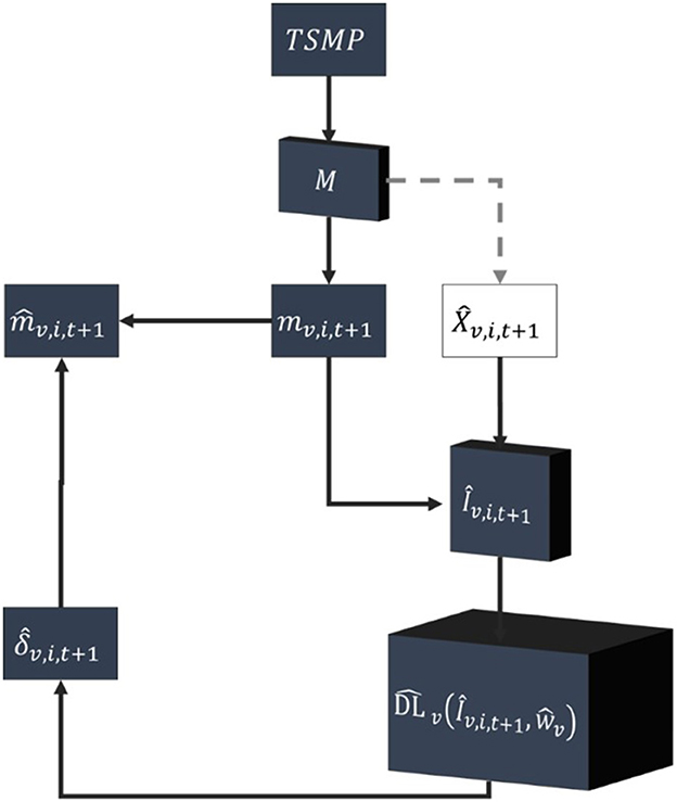
Figure 2. A schematic example of how the fully trained DL network and optimized inputs Î_{v, i, t+1}, can be used to predict ${\widehat{\delta }}_{v,i,t+1}$ for correcting the model forecast M_{v, i, t+1} at t+1.

2.3. Quantile mapping as a baseline method

We use empirical non-parametric quantile mapping (QM) as a baseline method to be compared with the results obtained by the DL-based method. Empirical QM is based on a transfer function for fitting the empirical historical model and reference CDFs ($f_{m_v}^{}$ and $f_{m_v}^{}$). The assumption in traditional QM is that the characteristics of $f_{m_v}^{}$ and $f_{r_v}^{}$ are stationary and do not change in the future (Cannon et al., 2015). The gamma function is a commonly used method for deriving empirical CDFs, especially for precipitation (Piani et al., 2010). However, we opted for a non-parametric approach to establish transfer functions that do not require specific assumptions on the distribution of the original data (i.e., precipitation and surface pressure). Empirical non-parametric QM has been shown to be effective in bias correction and can better capture non-linearities in the data (Tong et al., 2021).

Within the given context, the corrected model-based data in the forecast realm ${\widehat{m}}_{v,i,t}$ would be obtained as follows:

$\begin{array}{ll}{\widehat{m}}_{v,i,t}=f_{r_v}^{-1}\left\{f_{m_v}^{}(m_{v,i,t})\right\}& (9)\end{array}$

where v, i, and t represent the variable, space, and time indices. For quantile–quantile mapping (between $f_{m_v}^{-1}$ and $f_{r_v}^{-1}$), we compare linear, quadratic, and cubic regression and two cubic splines with different smoothness parameters for each variable. The information regarding the training, validation, and testing of QM is given in Section 2.6.

2.4. Study area and data

The proposed methodology is implemented over the European continent, where TSMP-G2A and COSMO-REA6 data are available. The study area consists of two domains, the global domain and the focus domain, which follow the predefined PRUDENCE regions (Christensen and Christensen, 2007). The UNet network is designed, such that it obtains the input information from the global domain and optimizes the loss function only over the focus domain. The reason for optimizing the loss function in the PRUDENCE regions is to exploit as much input information as possible from the global domain while avoiding boundary effects in the UNet network.

The global domain consists of 400 × 400 pixels cropped from the central part of the EUR-11 domain, according to the COordinated Regional Downscaling EXperiment (CORDEX) project (Giorgi et al., 2009; Jacob et al., 2014). The EUR-11 coordinate system is based on rotated latitude–longitude gridding with a horizontal resolution of 0.11 (12.5 km). The choice of a square-shaped study domain was made for convenience (e.g., obtaining images with even dimensions in max-pooling layers in UNet architecture).

The PRUDENCE regions are eight different geographical regions over the European continent represented in Figure 3 as red boxes (BI, British Isles; IB, Iberian Peninsula; FR, France; ME, mid-Europe; SC, Scandinavia; AL, Alps; MD, Mediterranean; EA, Eastern Europe).

FIGURE 3

Figure 3. Elevation map representing the global and focus domain in this study. The global domain consists of 400 ^* 400 pixels from the EUR-11 domain. The focus domain consists of 8 geographical regions named as Prudence regions.

The model-based precipitation and pressure data used in this study are obtained from the daily averaged simulation data (precipitation and surface pressure) of physically consistent Terrestrial Systems Modeling Platform (TSMP) over Europe (Gasper et al., 2014; Shrestha et al., 2014; Kollet et al., 2018). TSMP is a scale-consistent fully coupled terrestrial model comprising variables from the subsurface across the land surface to the top of the atmosphere. TSMP utilizes the external OASIS3 coupler (Valcke, 2013) for coupling the COSMO atmospheric model (Doms and Baldauf, 2012), CLM land model (Oleson et al., 2008), and ParFlow subsurface model (Kollet and Maxwell, 2006).

TSMP-G2A data provided by Furusho-Percot et al. (2019) offer an opportunity for studying feedback of states and fluxes of the water and energy cycle between the top of the atmosphere and down to groundwater. The ERA-Interim reanalysis was used as the boundary condition in the development of the TSMP-G2A simulations in 1979–2018. In the 1979–1989 spin-up period, groundwater–land surface subsystem was simulated with ParFlow-CLM using atmospheric forcing derived from ERA-Interim. The model was run transiently from January 1989 to August 2018 to allow the feedback process to evolve freely, and no data assimilation of any type of observation was included (Furusho-Percot et al., 2019). This “big” dataset is also potentially useful for developing/experimenting with the data-driven method because of its high volume (e.g., long time series and high resolution) and variety (e.g., fully interactive states and fluxes). For example, Ma et al. (2020, 2021) used TSMP-G2A to extract long-term memory correlations using deep learning to predict groundwater table depth anomalies, using precipitation and soil moisture information.

The spatial resolution and the domain of TSMP-G2A data match the EUR-11 CORDEX definition (rotated grid, 0.11). Data consist of physically driven atmospheric, land, surface, and subsurface information. This dataset is applied to this study due to its consistency with the reference data in terms of domain, gridding, and variable availability. Daily precipitation and surface pressure data for the years 1995–2017 are used from the TSMP-G2A data.

Atmospheric reanalysis data are gridded, spatiotemporal data of long-term estimates of climate variables. Reanalysis data are generated by using an NWP model and DA, which keeps the model-based data as close to the observations as possible while maintaining physical consistency. The reanalysis-based precipitation and surface pressure data in this study were obtained from the COSMO-REA6 atmospheric reanalysis product (Hu and Franzke, 2020), provided by the Hans Ertel Centre for Weather Research of the German Weather Service. The domain of this dataset matches the EURO-11 coordinate systems with a spatial resolution of 0.055 from 1995 to 2017. To ensure consistency in the comparison and calculation of mismatches between the model-based and reference data, the spatial resolution of the COSMO-REA6 was upscaled to 0.11 via simple averaging. There is no single precipitation dataset that is reliable for all regions and time scales. While reanalysis datasets generally show larger discrepancies compared to other datasets on a global scale (Sun et al., 2018), COSMO-REA6 captures precipitation patterns and intensity better than the global reanalysis ERA-Interim and the observational gridded dataset E-OBS in regions with low station density, especially in complex terrain (Kaiser-Weiss et al., 2019). Here, we used the COSMO-REA6 reanalysis data as an example reference data because it is continuous in space and time and compatible with TSMP-G2A in terms of domain, grid, and variable availability.

2.5. DL network setup

In the DL framework, we utilized a convolutional neural network (CNN). In contrast to other artificial neural networks, CNNs can efficiently utilize the complete information in space and time from the spatiotemporally correlated precipitation and pressure data sets, constituting an important feature of CNNs (Sadeghi et al., 2019). Thus, CNN is expected to be able to differentiate between different precipitation types considering the distinct correlation structure at individual and surrounding pixels.

A type of encoder–decoder CNN architecture, namely, UNet CNN by Ronneberger et al. (2015), was adapted and used in this study (Figure 4). While UNet has been proposed initially for biomedical image segmentation, several studies have recently modified and successfully used UNet for various applications in geosciences. UNet consists of down-sampling steps followed by symmetric up-sampling. The down-sampling steps capture the image context, and the up-sampling step is for precise localization of the features. Several hyperparameter settings were applied and tested in a trial-and-error manner (not shown). The final hyperparameter settings used are shown in Table 1.

FIGURE 4

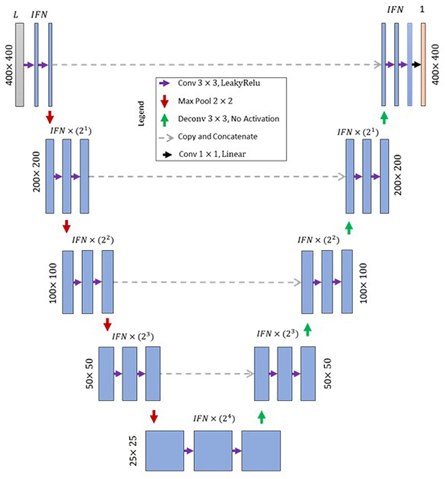
Figure 4. UNet model structure used in this study. Number of input layers in the model corresponds to the number of input members (L_{v, i, t} = |I_{v, i, t}|−1), IFN, Initial filter numbers, Conv, Convolutional layer, Max Pool, Max pooling layer, Deconv, Transposed convolution layer.

TABLE 1

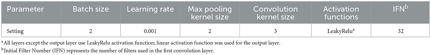
Table 1. Hyperparameter settings of the proposed UNet.

The UNet has two important properties: translation invariance and receptive field. The former property means that the network can recognize patterns in an image regardless of their location or pattern within the image. This is achieved using pooling layers. The receptive field property means that the network's prediction at a target location is fully determined by the input variables in a certain neighborhood, called the receptive field. Both properties are desirable as they counteract overfitting, but they also represent constraints (Tesch et al., 2023). For example, in this context, translation invariance can cause the network to overlook features that are not invariant to translation, and the receptive field can limit the network's ability in capturing dependencies between distant regions. To address this, we included orography information to provide context to the network regarding the orographic features of the pixels in the receptive field and the study area. This can help compensate for the limitations of these properties and result in improved performance for tasks that require spatiotemporal information.

The UNet structure is well known for its good performance in extracting features in analyzing spatial information (or images). However, the structure itself does not explicitly facilitate the extraction of temporal features unless it is fused with another structure (e.g., LSTM), to learn long-term temporal dependencies (Shi et al., 2015; Azad et al., 2019). As suggested in the literature, it is possible to leverage temporal information in the UNet model by considering various temporal lags (e.g., t−1, t−2) of input data (Sun et al., 2019; Teimouri et al., 2019; Bastos et al., 2021) or adding calendar information to UNet-shaped networks (Bastos et al., 2021).

We trained and tested various DL networks given various combinations of input data, I_{v, i, t}. In these combinations, we considered a 1-day lag of model-based data and calendar variables as well as orography. Orography includes time-independent images providing information about the longitude, latitude, and altitude of each corresponding pixel. Calendar data provide information about the Julian year and the day of the year of the input data given at time t. Each combination of I_{v, i, t} is unique because of different X_{v, i, t} sets. A list of training experiments and different combinations of input information is presented in Table 2.

TABLE 2

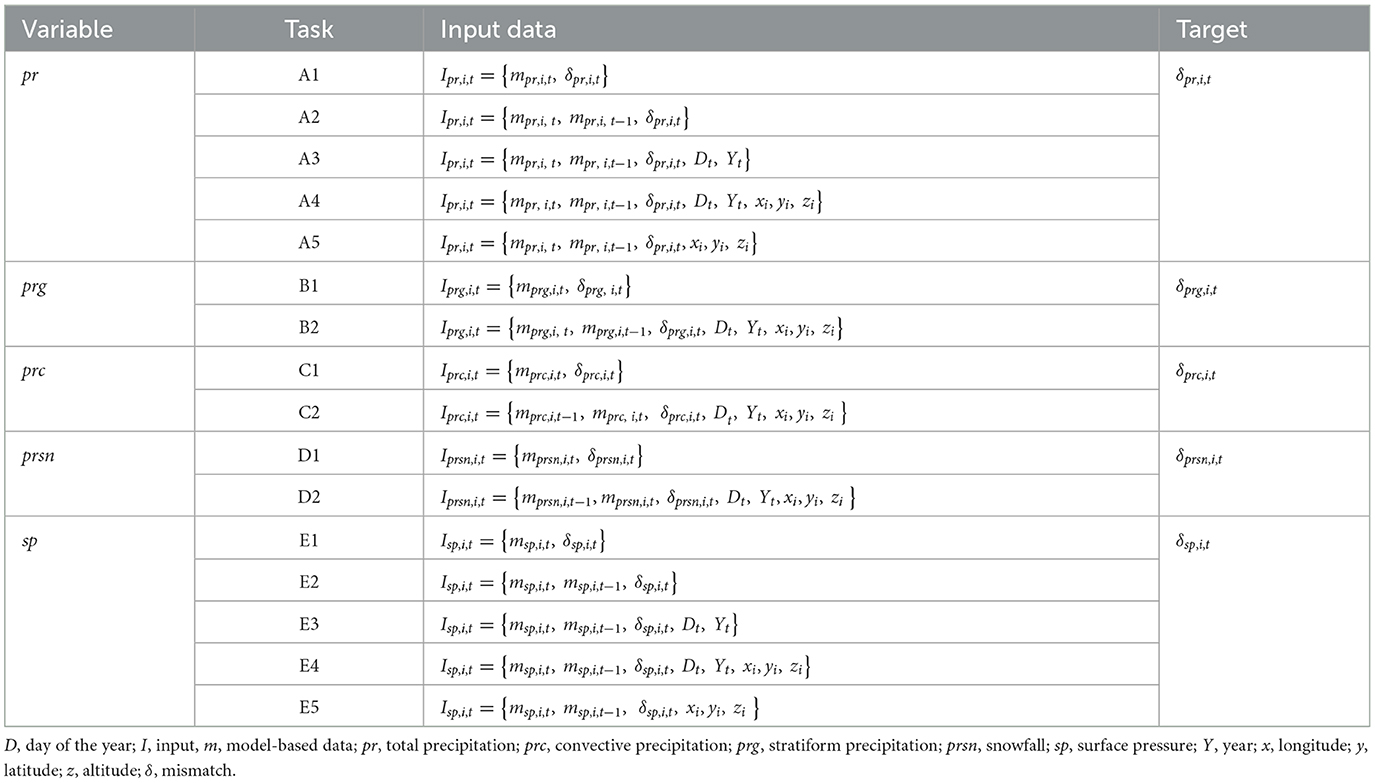
Table 2. Prediction tasks with different combinations of input data.

2.6. Training and validating the prediction tasks

For all tasks shown in Table 2, the data from 1995 to 2009 (5,475 days) were used for training the network, while the data from 2010 to 2014 (1,825 days) were used for validation. The data from 2015 to 2017 (1,095 days) were applied for independent testing. For network training, the data were normalized using the batch normalization function before every double-convolutional layer.

For training DL_v, all pixel information from the global region consisting of 400 × 400 pixels was provided to the network as image data in L_{v, i, t} layers. To avoid the boundary effects from boundary pixels, the loss function of the network was set to minimize Mean Squared Error (MSE) between ${\widehat{\delta }}_{v,i,t}$ and δ_{v, i, t} only over the focus region. In each epoch, errors representing the focus region were calculated for training and validation data.

The loss function is defined as the Mean Squared Error (MSE) of the data during the training period in the focus region as follows:

$\begin{array}{ll}MS{E}_{v,T}=\frac{1}{N_F{N}_T}{\displaystyle \sum _{t=1}^{N_T}}{\displaystyle \sum _{i=1}^{N_F}}({\widehat{\delta }}_{v,i,t}-{\delta }_{v,i,t}){}^2& (10)\end{array}$

where MSE_{v, P} represents the loss for variable v during the training period; N_F represents the number of pixels corresponding to the focus region; N_T represents the number of days in the training period; and ${\widehat{\delta }}_{v,i,t}$ and δ_{v, i, t} represent the predicted and measured mismatches.

The same error was calculated for the validation period as follows:

$\begin{array}{ll}MS{E}_{v,V}=\frac{1}{N_F{N}_V}{\displaystyle \sum _{t=1}^{N_V}}{\displaystyle \sum _{i=1}^{N_F}}({\widehat{\delta }}_{v,i,t}-{\delta }_{v,i,t}){}^2& (11)\end{array}$

where MSE_{v, V} represents the loss for variable v during the validation period and N_V represents the number of validation days.

In the keras and Tensorflow open-source packages in Python, which were utilized in this study, the Adam optimizer with a learning rate of 0.001 was used to minimize the loss function. The training was stopped if there were no further reductions in the MSE_{v, V} for eight consecutive epochs (patience =8). The trained weights of the network during the epoch with the smallest MSE_{v, V} were stored for comparison with other trained networks with varying input information (Table 2). The best combination of input data for predicting mismatches for five variables presented in Table 2 was selected according to an average of training and validation MSE as follows:

$\begin{array}{ll}A{V}_v=\frac{1}{2}(MS{E}_{v,T}+MS{E}_{v,V})& (12)\end{array}$

For each variable, the input data in the task with the least AV_v were chosen as the best input data.

We followed the same procedure for training, validation, and testing the baseline method. To match the quantiles using Equation 9, we generate the quantiles of the model data and reference data ($f_{r_v}^{-1}$ and $f_{m_v}^{-1}$), based on the training data (i.e., historical data), and use the validation data to identify the best regression method as a transfer function. The testing data are then used to correct the model-based data using the best transfer function and compared with the best DL-based method.

After choosing the best input data for each variable, the weights of the best input data (or task) were used to predict ${\widehat{\delta }}_{v,i,t}$ for pr and sp. The corrected model-based data (${\widehat{m}}_{v,i,t}$) were calculated according to Equation 8. We used the mean error (ME), Pearson correlation coefficient (COR), and root mean squared error (RMSE) metrics to compare ${\widehat{\delta }}_{v,i,t}$ with δ_{v, i, t} and ${\widehat{m}}_{v,i,t}$ with r_{v, i, t}. In the following, we explain how these error metrics are calculated for the former, which also applies to the latter.

Mean error (ME) is used for showing the average bias as follows:

$\begin{array}{ll}M{E}_{v,i}={\displaystyle \sum _{t=1}^N}\frac{{\widehat{\delta }}_{v,i,t}-{\delta }_{v,i,t}}{N}& (13)\end{array}$

where ME_{v, i} is a map showing ME for each pixel in the focus region and variable v and N is the total number of days from 1 January 1995 to 31 December 2017.

Pearson correlation coefficient (COR) is used as a measure of the linear relationship between ${\widehat{\delta }}_{v,i,t}$ and δ_{v, i, t}. COR is determined according to the following equation:

$\begin{array}{ll}CO{R}_{v,i}=\frac{{\displaystyle {\sum }_{i=1}^N({\widehat{\delta }}_{v,i,t}-{\overline{\widehat{\delta }}}_{v,i})({\delta }_{v,i,t}-{\overline{\delta }}_{v,i})}}{\sqrt{{\displaystyle {\sum }_{i=1}^N{({\widehat{\delta }}_{v,i,t}-{\overline{\widehat{\delta }}}_{v,i})}^2}}\sqrt{{\displaystyle {\sum }_{i=1}^N{({\delta }_{v,i,t}-{\overline{\delta }}_{v,i})}^2}}};& (14)\end{array}$

where ${\overline{\widehat{\delta }}}_{v,i}$ and ${\overline{\widehat{\delta }}}_{v,i}$ represent temporal averages of ${\widehat{\delta }}_{v,i,t}$ and δ_{v, i, t}.

Root mean squared error (RMSE) is used as a measure for determining the average distance between ${\widehat{\delta }}_{v,i,t}$ and δ_{v, i, t} as follows:

$\begin{array}{ll}RMS{E}_{v,i}=\sqrt{\frac{{\displaystyle {\sum }_{i=1}^N({\widehat{\delta }}_{v,i,t}-{\delta }_{v,i,t}){}^2}}{N}}& (15)\end{array}$

3. Results and discussion

First, in Section 3.1, we compare the spatiotemporal distributions of m_v, r_v, and δ_v that are the model and reference data and their mismatches, respectively. In Section 3.2, we show the evaluation results of various networks trained with different input data and provide the best input data combination for predicting δ_v. In addition, we compare the actual and predicted mismatches, δ_v and ${\widehat{\delta }}_v$, obtained by the best-identified networks. Finally, in Section 3.3, we compare the reference data with the merged data from the correction of the original model results.

3.1. Spatiotemporal distribution of the mismatches

Figures 5, 6 present the spatial distribution of long-term seasonal averages of the model and reference data and their mismatches for surface pressure (${\overline{m}}_{sp}$, ${\overline{r}}_{sp}$ and ${\overline{\delta }}_{sp}$, Figure 5) and total precipitation (${\overline{m}}_{pr}$, ${\overline{r}}_{pr}$ and ${\overline{\delta }}_{pr}$, Figure 6). The overbars indicate the averages calculated for each pixel based on daily values from 1995 to 2017 for DJF (December, January, and February, Figures 6A–D), MAM (March, April, and May, Figures 6E–H), JJA (June, July, and August, Figures 6I–L), and SON (September, October, and November, Figures 6M–P). The averages ${\overline{\delta }}_v$ are illustrated as seasonal maps and probability density distributions.

FIGURE 5

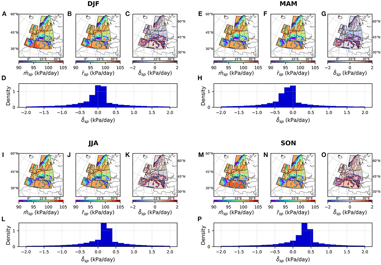
Figure 5. Seasonal maps of ${\overline{m}}_{sp}$ (A, E, I, M), ${\overline{r}}_{sp}$ (B, F, J, N), and ${\overline{\delta }}_{sp}$ (C, G, K, O), and the probability distribution of ${\overline{\delta }}_{sp}$ (D, H, L, P).

FIGURE 6

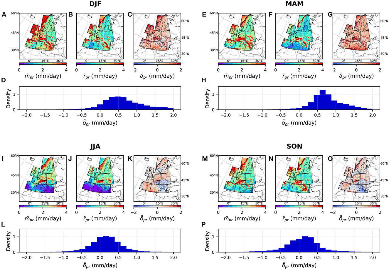
Figure 6. Same as Figure 5, but for pr.

According to Figures 5, 6, there is an overall underestimation of ${\overline{m}}_{sp}$ during MAM season, overestimation during JJA and SON seasons, and overestimation of ${\overline{m}}_{pr}$ during all seasons. A significant amount of this positive mismatch in total precipitation during all seasons is attributed with stratiform rainfall. Moreover, there is an underestimation of convective rainfall during JJA and SON seasons. In addition, topographical effects can be observed in both variables with strong positive or negative mismatches in higher altitudes.

The same figures for precipitation components (i.e., stratiform rainfall, convective rainfall, and snowfall) are provided in Supplementary material S1. Inspecting the different precipitation components, there is a clear positive bias, where ${\overline{m}}_{prg}$ accounts for a substantial amount of the overestimation (Supplementary Figure 1). On the other hand, ${\overline{m}}_{prc}$ appears to underestimate convective rainfall occurrence in Europe throughout JJA and SON months (Supplementary Figure 2). Moreover, there is a general overestimation of ${\overline{m}}_{prsn}$ during DJF months (Supplementary Figure 3).

3.2. Evaluation of the training and validation results

Table 3 represents the training and validation results of the different DL tasks presented in Table 2. According to Table 3, including spatiotemporal information as input layers (e.g., orography and calendar) yields an improvement (i.e., reduction in AVv ) compared against tasks with no additional input data. The improvement percentages range from 1.2% to 14% depending on the type of precipitation. For example, the prediction of δ_prsn has the greatest improvement of 14% when all the additional input data are included. We believe that this is due to the fact that snowfall mismatch prediction is more influenced by spatiotemporal seasonality. In general, the improvement in total precipitation is 3.9%. We tested the performance of the network by adding more model-based data from earlier time steps (i.e., t−2, t−3), which did not further improve the results (not shown here). The results obtained in Table 3 helped us understand the effectiveness of introducing spatiotemporal information for different types of precipitation. However, the following results in the manuscript pertain solely to total precipitation and surface pressure.

TABLE 3

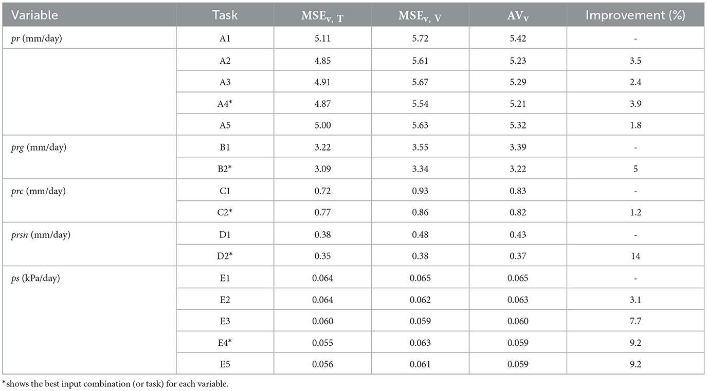
Table 3. Errors for DL tasks labeled according to various input datasets defined in Table 2.

We evaluated in detail the total precipitation (A4) and surface pressure (E4) from Table 3. The predicted mismatch data (${\widehat{\delta }}_{sp}$and ${\widehat{\delta }}_{pr}$) obtained by these two tasks were used for model-based data correction. The trained network weights in these tasks were used to generate ${\widehat{\delta }}_{sp}$and ${\widehat{\delta }}_{pr}$ for both training-validation and testing periods. In an ensuing step, the results are evaluated against the measured mismatches (δ_sp and δ_pr).

For the baseline method, we evaluated the validation results using the RMSE of various methods for fitting the quantile–quantile datapoints between TSMP-G2A and COSMO-REA6. Figure 7 is a comparison of the precipitation. According to the validation results, cubic regression (Figure 7D) has the best fit between the model-based and reference data quantiles. We used the same principle for surface pressure (Supplementary Figure 4) and cubic spline with a smoothing factor of s = 5 which had the best validation result. The two mentioned methods were used to generate TSMP-QM (corrected TSMP-G2A using QM) for precipitation and surface pressure.

FIGURE 7

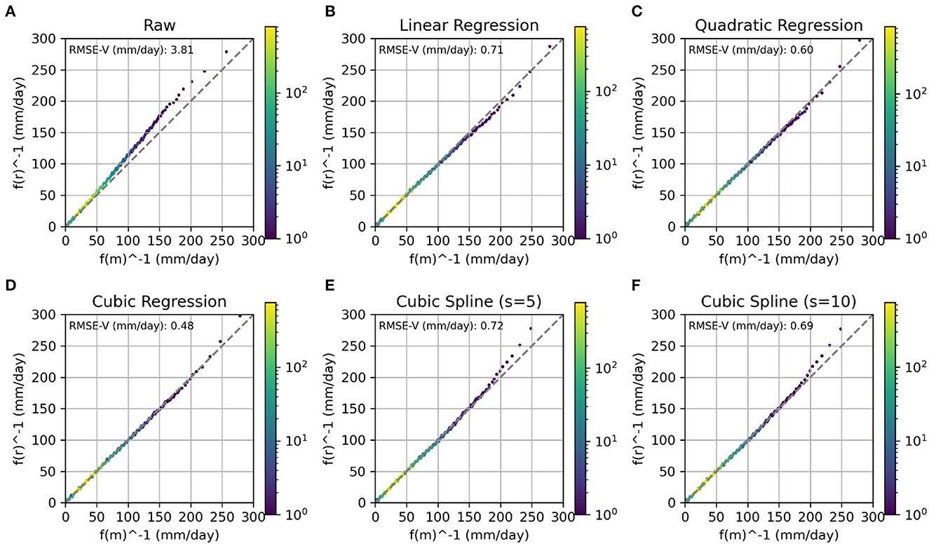
Figure 7. Comparison of quantile-quantile transfer functions for QM using the validation data for precipitation (v = pr). RMSE-V is calculated for validation data between f_rv−1 and f_mv−1 fitted using various methods (B–F) against the raw dataset (A).

Figure 8 shows the UNet skill in mismatch prediction for pr and sp over four seasons. The left column (Figures 8A–D, I–L) in these figures illustrates the probability density, and the right column (Figures 8E–H, M–P) represents the scatter plots of the seasonal averages of measured (${\overline{\delta }}_v$) and predicted (${\overline{\delta }}_v$) mismatches. According to the scatter plots, UNet's performance in predicting negative ${\overline{\widehat{\delta }}}_{pr}$ is limited. During the DJF and MAM months, ${\overline{\widehat{\delta }}}_{pr}$ vs. ${\overline{\delta }}_{pr}$ distributions match reasonably well. During JJA and SON months, however, with increasing convective rainfall (see Supplementary Figures 2J, N), the discrepancy in the distribution of predicted vs. measured mismatches is more pronounced.

FIGURE 8

Figure 8. Probability distribution (A–D) for pr, (I–L) for sp and scatter plots (E–H) for pr, (M–P) for sp for seasonal averages of predicted vs. measured mismatches (${\overline{\delta }}_v$ vs. ${\overline{\delta }}_v$).

Figures 9, 10 show the seasonally averaged spatial distribution of RMSE and COR between ${\overline{\widehat{\delta }}}_v$ and ${\overline{\delta }}_v$. According to Figure 9, ${\overline{\widehat{\delta }}}_{sp}$ has the highest RMSE and COR during MAM months (Figures 9C, D) and the lowest RMSE and COR during JJA and SON months (Figures 9E–H), respectively. Unlike sp, the orography plays a significant role in the UNet prediction skill for pr. For example, from Figure 10, the majority of the highest RMSE values correspond to the Scandinavian highlands and Alps. Additionally, there is a shift in the higher RMSE and lower COR values toward the south of central and northern Europe from JJA to SON months, which is attributed to the prevalence of convective precipitation in these regions during these seasons.

FIGURE 9

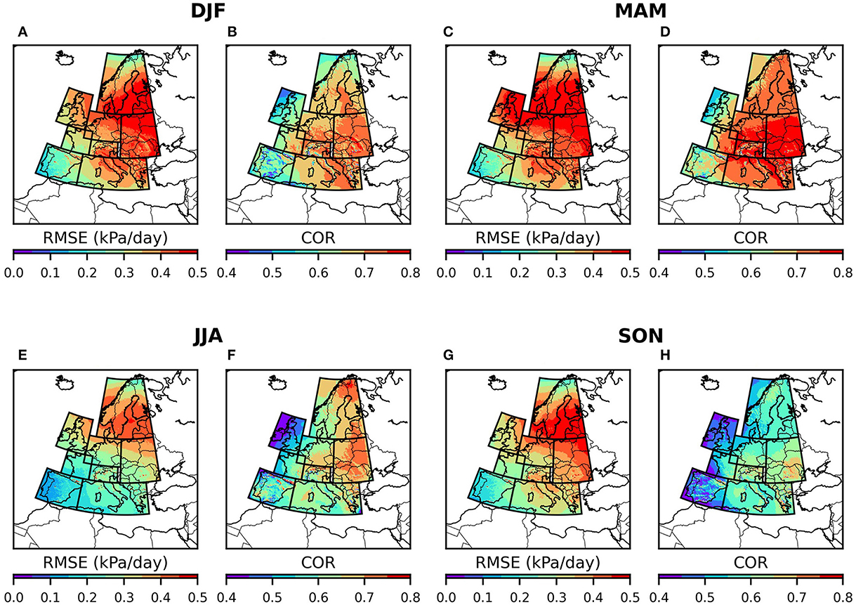
Figure 9. Spatio-temporal distribution of RMSE (A, C, E, G) and COR (B, D, F, H) of surface pressure ${\widehat{\delta }}_{sp}$ against δ_sp.

FIGURE 10

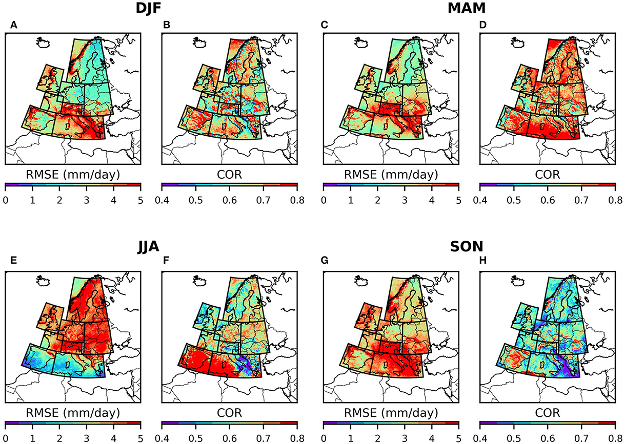
Figure 10. Same as Figure 8, but for pr.

UNet CNN was shown to capture precipitation and surface pressure mismatch information over the focus region with an average correlation coefficient of 0.65 and 0.63, respectively. Therefore, it appears that UNet can predict the mismatches leading to a general reduction in bias and improving model accuracy. Nonetheless, the mismatch distributions depicted are temporally averaged, and extreme events were not explored independently. Thus, further research is required to evaluate the applicability of the framework for the correction of extreme events.

3.3. Evaluation of the testing results

Here, we focus only on the testing data (2015–2017), which have not been used either to determine the weights in the UNet or to generate the empirical quantiles and transfer functions in QM. We compare the performances of original model-based data (TSMP-G2A) against TSMP-QM (model-based data corrected using QM) and TSMP-UNET (model-based data corrected using UNet). Table 4 contains statistics related to precipitation (pr) and surface pressure (sp) for the aforementioned data. The table displays ME, COR, and RMSE and the overall spatiotemporal average value obtained from COSMO-REA (shown with AV) over various seasons.

TABLE 4

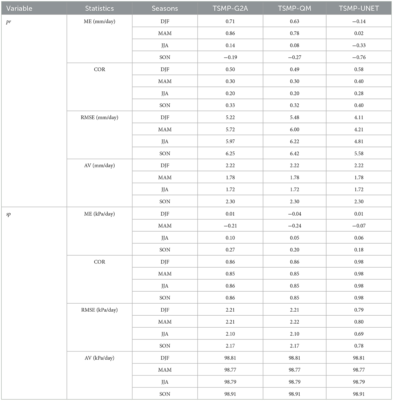
Table 4. Testing evaluation results given for TSMP-G2A, TSMP-QM, and TSMP-UNET data over various seasons for pr and sp.

Table 4 suggests that TSMP-UNET outperforms TSMP-QM in terms of RMSE and COR in precipitation and surface pressure. While TSMP-QM performs better than TSMP-UNET in closing the ME gap during JJA and SON months for precipitation and during JJA months for surface pressure, other metrics favor TSMP-UNET. Gap reduction in ME compromises other error metrics (i.e., COR and RMSE), which is a well-known tradeoff in bias correction. The compromise is reflected more in QM than UNet for precipitation and corresponds with the findings of previous studies that have compared traditional bias correction methods over DL (Hess and Boers, 2022). The uncertainty in summertime precipitation (e.g., convective rainfall) makes it more challenging for both methods to reduce the average error and the dispersion of the error. This is reflected in worse RMSE values of TSMP-QM precipitation and no changes in RMSE of TSMP-QM surface pressure.

3.4. Evaluation of TSMP-UNET

After generating the corrected model-based data (${\widehat{m}}_{v,i,t}$, Equation 8), TSMP-G2A and TSMP-Unet were compared with COSMO-REA6. Figures 11, 12 show the spatial distribution of various error statistics (ME, ESD, RMSE, and COR) for TSMP-G2A (Figures 11A–C, 12A–C), ${\widehat{m}}_{v,i,t}$ (Figures 11D–F, 12D–F), and the relative percentage of improvement against the original model-based data (Figures 11G–I, 12G–I).

FIGURE 11

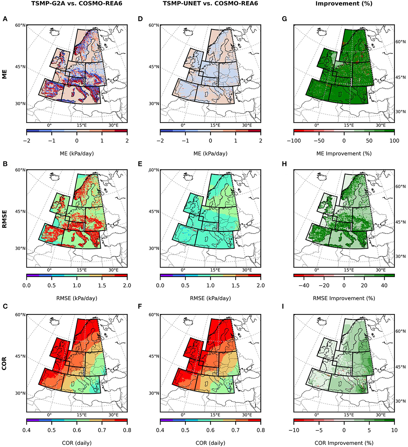
Figure 11. Maps of average Mean Error (ME), Root Mean Squared Error (RMSE), and Correlation Coefficient (COR) calculated for TSMP-G2A (A-C), and TSMP-UNET (D-F) against COSMO-REA6, and the percentage of improvement (G-I) for sp.

FIGURE 12

Figure 12. The same as Figure 11, but for pr.

Figures 11, 12 show that the application of the predicted mismatches strongly improves the estimates of precipitation and surface pressure resulting in a decrease in ME and RSME and an increase in COR almost in all regions. Interestingly, there are locations where the merger impacts the ME negatively (Figures 11G, 12G). In addition, there are areas where UNet predictions have a small effect on reducing RMSE in precipitation compared to surface pressure (Figure 11H). In these cases, the complex and chaotic nature of convective and orographic precipitation adds a strong random component to the model and reference data, in which UNet is apparently not able to capture in the training.

In Figures 13, 14, the monthly time series of regional averages of TSMP-G2A, COSMO-REA6, and ${\widehat{m}}_{v,i,t}$are shown for the PRUDENCE focus regions. In both figures, the years between 1995 and 2010 correspond to training, between 2010 and 2015 correspond to validation, and between 2015 and 2017 correspond to testing. In general, ${\widehat{m}}_{v,i,t}$shows a good agreement with COSMO-REA6, which is generally consistent in all training, validation, and testing periods. However, a limitation is over-correction or under-correction effects that can be observed in the peaks in the time series (Figure 14B). However, the merged product's daily and monthly aggregated results show an improvement compared to the original model results. On average, for pr and sp, ${\widehat{m}}_{v,i,t}$ is improved significantly (47% reduction in ME, 37% increase in daily COR, and 22% reduction in RMSE). The added utility of this approach is not only limited to one model compartment. In addition, the benefits obtained by an online correction of atmospheric variables (${\widehat{m}}_{v,i,t}$) in an integrated terrestrial modeling platform, such as TSMP, will also yield improvements in the states of other terrestrial compartments of the model (e.g., surface/subsurface variables).

FIGURE 13

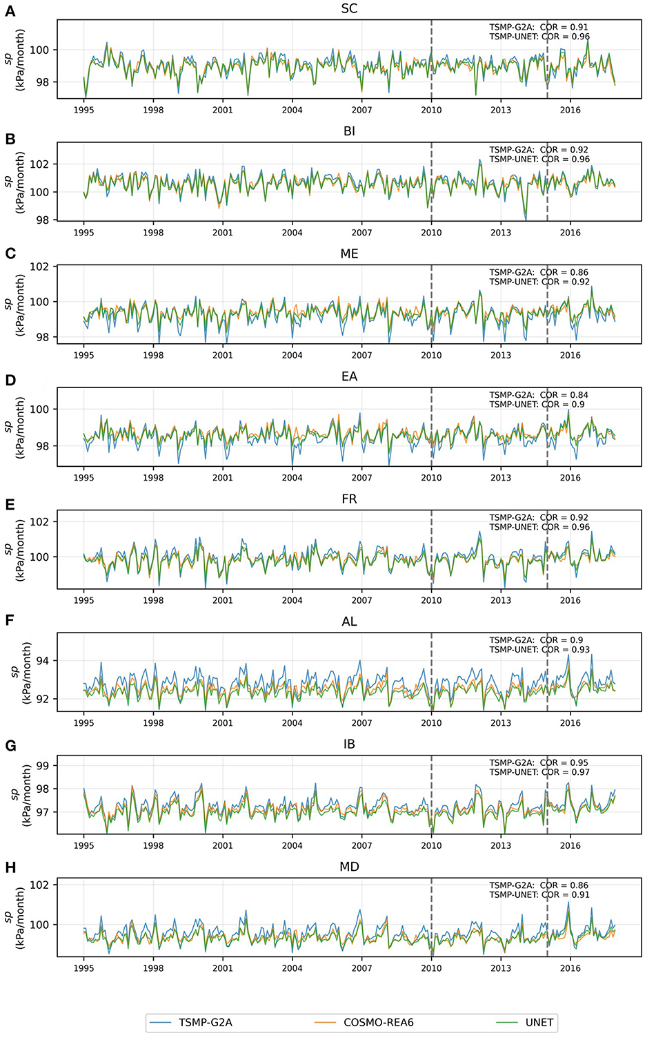
Figure 13. Time-series of monthly average surface pressure (sp) for TSMP-G2A, COSMO-REA6, and TSMP-UNET data over different regions (A–H).

FIGURE 14

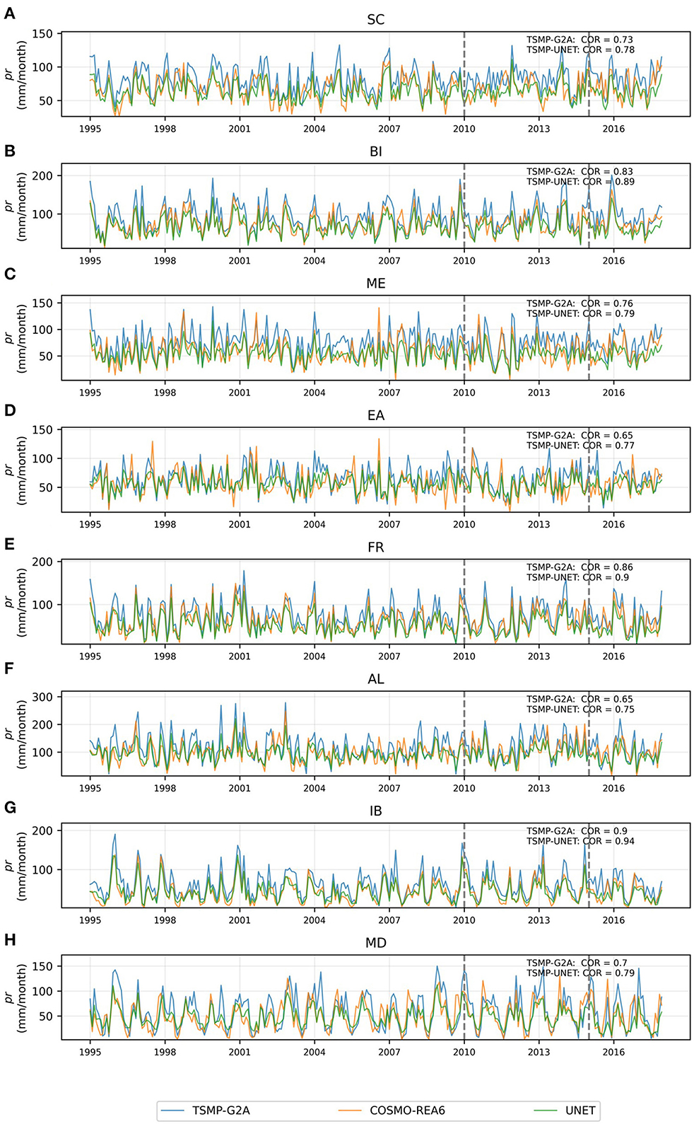
Figure 14. Time-series of monthly average total precipitation (pr) for TSMP-G2A, COSMO-REA6, and TSMP-UNET data over different regions (A–H).

4. Conclusion

In this study, we applied a previously proposed method to atmospheric variables based on the rationale to arrive at a correction method for online hydrologic/impact simulations in earth system modeling. A DL network, UNet CNN, was designed to learn mismatches between a set of model and reference data by using the model-based data as the main input and varying additional input data including topographical and temporal information. According to the proposed DL-based merging methodology, the predicted mismatch data obtained by the best UNet network were used to correct the model-based data. To investigate the improvements in the original model-based data, we compared the corrected data (TSMP-UNET) and original model-based data (TSMP-G2A) with the reanalysis-based data (COSMO-REA6). Assuming COSMO-REA6 represents the “ground truth” data, it is possible to utilize the network weights learned by the DL network in conjunction with the physically based model information from TSMP to arrive at an improved forecast of precipitation, surface pressure, or potentially any atmospheric and hydrologic variable, in general, which needs to be demonstrated in future studies.

Comparing TSMP-UNET and TSMP-G2A with COSMO-REA6 data shows significant improvements in the original model-based data across most grid cells in the focus domain. The mean error (ME), root mean square error (RMSE), and Pearson correlation coefficient (COR) values of TSMP-UNET data have improved substantially. However, it is worth noting that in some oceanic regions, applying predicted mismatches from UNet leads to a deterioration of ME values, as shown in Figure 12G. This may be due to differences in precipitation characteristics over land and ocean caused by differences in the assimilation of prognostic variables in COSMO-REA6. Similar problems occur for convective precipitation mainly in SON and JJA months. Although UNet can reduce both error dispersion and mean error across all seasons, it may worsen mean error during SON and JJA months. This can be due to the translation invariance property of the UNet. The inclusion of spatiotemporal information in the inputs has improved UNet's performance, but convective rainfall remains highly variable and independent of the provided spatiotemporal information, making it difficult to improve UNet's performance in comparison to snowfall. While training separate UNet models for land and ocean may be a viable solution, a single network that can suppress all error metrics over all regions and seasons is currently not feasible for precipitation. Despite these challenges, the DL-based merging framework has shown potential for improving atmospheric variables beyond the two examples studied.

Deep learning of mismatches from a more chaotic variable, such as precipitation, appears to be more challenging than a less chaotic variable, such as surface pressure. Precipitation is non-Gaussian, right-skewed, and highly variable over space and time as well as in intensity and duration. One of the challenges in dealing with precipitation is in detecting the negative mismatches (Figures 7G, H). Negative mismatches occur when there is no or less amount of precipitation in the model-based data, while there is an arbitrary amount of precipitation in the reference data. Models often lack sensitivity in triggering precipitation. Therefore, it can be challenging for the neural network to learn negative mismatches since the model-based data are the main input data used for predicting the mismatches. One area of improvement can be the use of ensemble model data (i.e., using various simulation data out of the same model or different models) so that the information provided by each model as input data in the DL network can compensate for failure or lack of information in the input data. However, when comparing the correlation coefficient obtained by predicted mismatches for these two variables, the correlation coefficient results are similar (roughly 0.65). This might be an indication of the lack of temporal information extracted in the UNet architecture used in this study. Furthermore, introducing calendar information as an additional variable improved the network's performance slightly (2.4% reduction in loss function for precipitation and 7.7% for surface pressure). This suggests that a DL network (e.g., ConvLSTM or 3D Conv) that better uses the temporal information would have the ability to learn the mismatches with a higher prediction skill. The main advantage gained by utilizing reanalysis data as the reference data is the spatiotemporal continuity, which is useful in quantifying the mismatch structure at every point in time and space. However, the accuracy of the reanalysis data is limited and often is validated against the available observed data due to their higher accuracy and consistency in representing the ground truth. Utilizing observations as reference data can provide more accurate and consistent “ground truth” information for the DL network to learn from. However, observations have other limitations such as sparse spatial coverage, incomplete temporal coverage, and data processing errors. Both reanalysis and observation data have their own advantages and limitations, and their usage in the DL network depends on the specific research questions and the availability and quality of the data.

By using the DL-based merging as a post-processor to correct the atmospheric simulations, the accuracy of the land surface model can be improved. Additionally, comparing the simulation data from the land surface model with in situ measurements can indirectly validate the effectiveness of the DL-based merging technique. This approach can potentially lead to more accurate predictions of water resources, crop yields, and other environmental variables, which can have significant implications for decision-making in areas such as agriculture, water management, and disaster preparedness.

Data availability statement

Refer to Bollmeyer et al. (2015) and Furusho-Percot et al. (2019) for accessing the raw data (original TSMP-G2A and COSMO-REA6) used in this study. The preprocessed and mismatch data are made available (Yousefi and Kollet, 2022).

Author contributions

KP and SK contributed to the conception and design of the study. KP conducted all the experiments and analyzed the results with feedback from SK. KP prepared the draft manuscript with contributions from SK. Both authors contributed to the article and approved the submitted version.

Funding

This study received funding from the K1:STE project [grant no: 67KI2043] in association with the German Federal Ministry for the Environment, Nature Conservation, Nuclear Safety, and Consumer Protection (BMUV).

Acknowledgments

The authors gratefully acknowledge the computing time granted through the ESM and DEEPACF projects on the JUWELS supercomputer at the Jülich Supercomputing Center (JSC).

Conflict of interest

The authors declare that the research was conducted in the absence of any commercial or financial relationships that could be construed as a potential conflict of interest.

Publisher's note

All claims expressed in this article are solely those of the authors and do not necessarily represent those of their affiliated organizations, or those of the publisher, the editors and the reviewers. Any product that may be evaluated in this article, or claim that may be made by its manufacturer, is not guaranteed or endorsed by the publisher.

Supplementary material

The Supplementary Material for this article can be found online at: https://www.frontiersin.org/articles/10.3389/frwa.2023.1178114/full#supplementary-material

References

Ayzel, G., Scheffer, T., and Heistermann, M. (2020). RainNet v1, 0. a convolutional neural network for radar-based precipitation nowcasting. Geoscien. Model Develop. Discuss. 3, 1–20. doi: 10.5194/gmd-2020-30

CrossRef Full Text | Google Scholar

Azad, R., Asadi-Aghbolaghi, M., Fathy, M., and Escalera, S. (2019). Bi-directional ConvLSTM U-net with densley connected convolutions. Proceedings - 2019 International Conference on Computer Vision Workshop, ICCVW 2019, 406–415. doi: 10.1109/ICCVW.2019.00052

CrossRef Full Text | Google Scholar

Bastos, B. Q., Cyrino Oliveira, F. L., and Milidiú, R. L. (2021). U-Convolutional model for spatio-temporal wind speed forecasting. Int. J. Forecast. 37, 949–970. doi: 10.1016/j.ijforecast.10007.

CrossRef Full Text | Google Scholar

Bollmeyer, C., Keller, J. D., Ohlwein, C., Wahl, S., Crewell, S., Friederichs, P., et al. (2015). Towards a high-resolution regional reanalysis for the european CORDEX domain. Quart. J. Royal Meteorol. Soc. 141, 1–15. doi: 10.1002/qj.2486

CrossRef Full Text | Google Scholar

Cannon, A. J., Sobie, S. R., and Murdock, T. Q. (2015). Bias correction of GCM precipitation by quantile mapping: How well do methods preserve changes in quantiles and extremes? J. Clim. 28, 6938–6959. doi: 10.1175/JCLI-D-14-00754.1

CrossRef Full Text | Google Scholar

Christensen, J. H., and Christensen, O. B. (2007). A summary of the PRUDENCE model projections of changes in European climate by the end of this century. Clim. Change, 81(SUPPL. 1), 7–30. doi: 10.1007./s10584-006-9210-7

CrossRef Full Text | Google Scholar

Déqué, M. (2007). Frequency of precipitation and temperature extremes over France in an anthropogenic scenario: Model results and statistical correction according to observed values. Glob. Planet. Change, 57, 16–26. doi: 10.1016/j.gloplacha.11030

CrossRef Full Text | Google Scholar

Doms, G., and Baldauf, M. (2012). Consortium for Small-Scale Modelling A Description of the Nonhydrostatic Regional COSMO-Model Part I : Dynamics and Numerics. Deutscher Wetterdienst, Offenbach. December, 93. doi: 10.5676./DWD

CrossRef Full Text | Google Scholar

Furusho-Percot, C., Goergen, K., Hartick, C., Kulkarni, K., Keune, J., Kollet, S., et al. (2019). Pan-European groundwater to atmosphere terrestrial systems climatology from a physically consistent simulation. Scient. Data, 6, 320. doi: 10.1038/s41597-019-0328-7

PubMed Abstract | CrossRef Full Text | Google Scholar

Gasper, F., Goergen, K., Shrestha, P., Sulis, M., Rihani, J., Geimer, M., et al. (2014). Implementation and scaling of the fully coupled terrestrial systems modeling platform (TerrSysMP v1.0) in a massively parallel supercomputing environment—A case study on JUQUEEN (IBM Blue Gene/Q). Geoscient. Mod. Develop. 7, 2531–2543. doi: 10.5194/gmd-7-2531-2014

CrossRef Full Text | Google Scholar

Geer, A. J. (2020). Learning Earth System Models Observations, Machine Learning or Data Assimilation? Available online at: http://www.ecmwf.int/en/publications (accessed December 14, 2020).

PubMed Abstract | Google Scholar

Giorgi, F., Jones, C., and Asrar, G. (2009). Addressing climate information needs at the regional level: the CORDEX framework. Organization (WMO) Bulletin, November 2008.

Google Scholar

Han, L., Chen, M., Chen, K., Chen, H., Zhang, Y., Lu, B., et al. (2021). A deep learning method for bias correction of ECMWF 24–240 h forecasts. Adv. Atmosph. Sci. 38, 1444–1459. doi: 10.1007/s00376-021-0215-y

CrossRef Full Text | Google Scholar

Hess, P., and Boers, N. (2022). Deep learning for improving numerical weather prediction of heavy rainfall. J. Adv. Model. Earth Sys. 14, 2765. doi: 10.1029/2021MS002765

CrossRef Full Text | Google Scholar

Holthuijzen, M., Beckage, B., Clemins, P. J., Higdon, D., and Winter, J. M. (2022). Robust bias-correction of precipitation extremes using a novel hybrid empirical quantile-mapping method: Advantages of a linear correction for extremes. Theoret. Appl. Climatol. 149, 863–882. doi: 10.1007/s00704-022-04035-2

CrossRef Full Text | Google Scholar

Hu, G., and Franzke, C. L. E. (2020). Evaluation of daily precipitation extremes in reanalysis and gridded observation-based data sets over Germany. Geophys. Res. Lett. 47, 624. doi: 10.1029./2020GL089624

CrossRef Full Text | Google Scholar

Ibebuchi, C. C., Schönbein, D., Adakudlu, M., Xoplaki, E., and Paeth, H. (2022). Comparison of three techniques to adjust daily precipitation biases from regional climate models over Germany. Water, 14, 600. doi: 10.3390./w14040600

CrossRef Full Text | Google Scholar

Jacob, D., Petersen, J., Eggert, B., Alias, A., Christensen, O. B., Bouwer, L. M., et al. (2014). EURO-CORDEX: new high-resolution climate change projections for European impact research. Reg. Environ. Change, 14, 563–578. doi: 10.1007/s10113-013-0499-2

CrossRef Full Text | Google Scholar

Kaiser-Weiss, A. K., Borsche, M., Niermann, D., Kaspar, F., Lussana, C., Isotta, F. A., et al. (2019). Added value of regional reanalyses for climatological applications. In Environmental Research Communications (Vol. 1, Issue 7). Institute of Physics. doi: 10.1088/2515-7620/ab2ec3

CrossRef Full Text | Google Scholar

Kollet, S., Gasper, F., Brdar, S., Goergen, K., Hendricks-Franssen, H. J., Keune, J., et al. (2018). Introduction of an experimental terrestrial forecasting/monitoring system at regional to continental scales based on the terrestrial systems modeling platform (v1, 1.0). Water, 10, 1697. doi: 10.3390/w10111697

CrossRef Full Text | Google Scholar

Kollet, S. J., and Maxwell, R. M. (2006). Integrated surface–groundwater flow modeling: a free-surface overland flow boundary condition in a parallel groundwater flow model. Adv. Water Res. 29, 945–958. doi: 10.1016/j.advwatres.08006

CrossRef Full Text | Google Scholar

Ma, Y., Montzka, C., Bayat, B., and Kollet, S. (2020). Using Long Short-Term Memory networks to connect water table depth anomalies to precipitation anomalies over Europe. Hydrol. Earth Sys. Sci. 25, 3555–3575. doi: 10.5194/hess-2020-382

CrossRef Full Text | Google Scholar

Ma, Y., Montzka, C., Bayat, B., and Kollet, S. (2021). An indirect approach based on long short-term memory networks to estimate groundwater table depth anomalies across Europe with an application for drought analysis. Front.Water 3, 1–13. doi: 10.3389./frwa.2021.723548

CrossRef Full Text | Google Scholar

Moghim, S., and Bras, R. L. (2017). Bias correction of climate modeled temperature and precipitation using artificial neural networks. J. Hydrometeorol. 18, 1867–1884. doi: 10.1175/JHM-D-16-0247.1

CrossRef Full Text | Google Scholar

Naz, B. S., Kurtz, W., Montzka, C., Sharples, W., Goergen, K., Keune, J., et al. (2019). Improving soil moisture and runoff simulations at 3andkm over Europe using land surface data assimilation. Hydrol. Earth Sys. Sci. 23, 277–301. doi: 10.5194/hess-23-277-2019

CrossRef Full Text | Google Scholar

Oleson, K. W., Niu, G. Y., Yang, Z. L., Lawrence, D. M., Thornton, P. E., Lawrence, P. J., et al. (2008). Improvements to the community land model and their impact on the hydrological cycle. J. Geophys. Res. Biogeosci. 113, 563. doi: 10.1029./2007J.G.000563

CrossRef Full Text | Google Scholar

Pan, B., Hsu, K., AghaKouchak, A., and Sorooshian, S. (2019). Improving precipitation estimation using convolutional neural network. Water Res. Res. 55, 2301–2321. doi: 10.1029/2018WR024090

CrossRef Full Text | Google Scholar

Panofsky, H. A., and Brier, G. W. (1968). Some Applications of Statistics to Meteorology. Earth and Mineral Sciences Continuing Education College of Earth and Mineral Sciences The Pennsylvania State University, University Park, Pennsylvania, PA, United States.

Google Scholar

Passow, C., and Donner, R. V. (2020). Regression-based distribution mapping for bias correction of climate model outputs using linear quantile regression. Stochastic Environ. Res. Risk Assess. 34, 87–102. doi: 10.1007/s00477-019-01750-7

CrossRef Full Text | Google Scholar

Piani, C., Haerter, J. O., and Coppola, E. (2010). Statistical bias correction for daily precipitation in regional climate models over Europe. Theoret. Appl. Climatol. 99, 187–192. doi: 10.1007/s00704-009-0134-9

CrossRef Full Text | Google Scholar

Prein, A. F., Langhans, W., Fosser, G., Ferrone, A., Ban, N., Goergen, K., et al. (2015). A review on regional convection-permitting climate modeling: demonstrations, prospects, and challenges. Rev. Geophys. 53, 323–361. doi: 10.1002/2014RG000475

PubMed Abstract | CrossRef Full Text | Google Scholar

Räisänen, J., and Räty, O. (2013). Projections of daily mean temperature variability in the future: cross-validation tests with ENSEMBLES regional climate simulations. Clim. Dynam. 41, 1553–1568. doi: 10.1007/s00382-012-1515-9

CrossRef Full Text | Google Scholar

Räty, O., Räisänen, J., and Ylhäisi, J. S. (2014). Evaluation of delta change and bias correction methods for future daily precipitation: intermodel cross-validation using ENSEMBLES simulations. Clim. Dynam. 42, 2287–2303. doi: 10.1007/s00382-014-2130-8

CrossRef Full Text | Google Scholar

Reichle, R. H. (2008). (2008). Data assimilation methods in the Earth sciences. Adv. Water Res. 31, 1411–1418. doi: 10.1016/j.advwatres.01001

CrossRef Full Text | Google Scholar

Ronneberger, O., Fischer, P., and Brox, T. (2015). U-net: convolutional networks for biomedical image segmentation. IEEE Access 9, 16591–16603. doi: 10.1109/ACCESS.2021.3053408

CrossRef Full Text | Google Scholar

Sadeghi, M., Asanjan, A. A., Faridzad, M., Nguyen, P. H. U., Hsu, K., Sorooshian, S., et al. (2019). PERSIANN-CNN: Precipitation estimation from remotely sensed information using artificial neural networks—Convolutional neural networks. J. Hydrometeorol. 20, 2273–2289. doi: 10.1175/JHM-D-19-0110.1

CrossRef Full Text | Google Scholar

Shi, X., Chen, Z., Wang, H., Yeung, D. Y., Wong, W. K., Woo, W. C., et al. (2015). Convolutional LSTM network: a machine learning approach for precipitation nowcasting. Adv. Neural Inf. Process. Syst. 2015, 802–810. doi: 10.48550/arXiv.1506.04214

CrossRef Full Text | Google Scholar

Shrestha, P., Sulis, M., Masbou, M., Kollet, S., and Simmer, C. (2014). A scale-consistent terrestrial systems modeling platform based on COSMO, CLM, and ParFlow. Month. Weath. Rev. 142, 3466–3483. doi: 10.1175/MWR-D-14-00029.1

CrossRef Full Text | Google Scholar

Sun, A. Y., Scanlon, B. R., Zhang, Z., Walling, D., Bhanja, S. N., Mukherjee, A., et al. (2019). Combining physically based modeling and deep learning for fusing GRACE satellite data: can we learn from mismatch? Water Resour. Res. 55, 1179–1195. doi: 10.1029/2018WR023333

CrossRef Full Text | Google Scholar

Sun, Q., Miao, C., Duan, Q., Ashouri, H., Sorooshian, S., Hsu, K. L., et al. (2018). A review of global precipitation data sets: data sources, estimation, and intercomparisons. Rev. Geophys. 56, 79–107. doi: 10.1002/2017RG000574

CrossRef Full Text | Google Scholar

Teimouri, N., Dyrmann, M., and Jørgensen, R. N. (2019). A novel spatio-temporal FCN-LSTM network for recognizing various crop types using multi-temporal radar images. Remote Sens. 11, 990. doi: 10.3390/rs11080990

CrossRef Full Text | Google Scholar

Tesch, T., Kollet, S., and Garcke, J. (2023). Causal deep learning models for studying the Earth system: soil moisture-precipitation coupling in ERA5 data across Europe. EGUsphere 17, 1–32. doi: 10.5194./egusphere-2022-105

CrossRef Full Text | Google Scholar

Tong, Y., Gao, X., Han, Z., Xu, Y., Xu, Y., Giorgi, F., et al. (2021). Bias correction of temperature and precipitation over China for RCM simulations using the QM and QDM methods. Clim. Dynam. 57, 1425–1443. doi: 10.1007/s00382-020-05447-4

CrossRef Full Text | Google Scholar

Valcke, S. (2013). The OASIS3 coupler: a European climate modelling community software. Geoscient. Model Develop. 6, 373–388. doi: 10.5194/gmd-6-373-2013

CrossRef Full Text | Google Scholar

Wahl, S., Bollmeyer, C., Crewell, S., Figura, C., Friederichs, P., Hense, A., et al. (2017). A novel convective-scale regional reanalysis COSMO-REA2: improving the representation of precipitation. Meteorol. Zeitschrift, 26, 345–361. doi: 10.1127/metz/2017/0824

CrossRef Full Text | Google Scholar

Yousefi, P. K., and Kollet, S. (2022). Data for: Deep Learning of Model- and Reanalysis- Based Precipitation and Pressure Mismatches over Europe. Zenodo [Preprint]. doi: 10.5281/zenodo.6873802

CrossRef Full Text | Google Scholar

Zhang, C. J., Zeng, J., Wang, H. Y., Ma, L. M., and Chu, H. (2020). Correction model for rainfall forecasts using the LSTM with multiple meteorological factors. Meteorol. Appl. 27, 1–15. doi: 10.1002/met.1852

CrossRef Full Text | Google Scholar