 Fang Li
 Wolfgang Kurtz1,2†
 Harry Vereecken
 Harrie-Jan Hendricks Franssen
- 1Agrosphere Institute, IBG-3, Forschungszentrum Jülich GmbH, Jülich, Germany
- 2Centre for High-Performance Scientific Computing in Terrestrial Systems: HPSC TerrSys, Geoverbund ABC/J, Leo-Brandt-Strasse, Jülich, Germany
As an important source of water for human beings, groundwater plays a significant role in human production and life. However, different sources of uncertainty may lead to unsatisfactory simulations of groundwater hydrodynamics with hydrological models. The goal of this study is to investigate the impact of assimilating groundwater data into the Terrestrial System Modeling Platform (TSMP) for improving hydrological modeling in a real-world case. Daily groundwater table depth (WTD) measurements from the year 2018 for the Rur catchment in Germany were assimilated by the Localized Ensemble Kalman Filter (LEnKF) into TSMP. The LEnKF is used with a localization radius so that the assimilated measurements only update model states in a limited radius around the measurements, in order to avoid unphysical updates related to spurious correlations. Due to the mismatch between groundwater measurements and the coarse model resolution (500 m), the measurements need careful screening before data assimilation (DA). Based on the spatial autocorrelation of the WTD deduced from the measurements, three different filter localization radii (2.5, 5, and 10 km) were evaluated for assimilation. The bias in the simulated water table and the root mean square error (RMSE) are reduced after DA, compared with runs without DA [i.e., open loop (OL) runs]. The best results at the assimilated locations are obtained for a localization radius of 10 km, with an 81% reduction of RMSE at the measurement locations, and slightly smaller RMSE reductions for the 5 and 2.5 km radius. The validation with independent WTD data showed the best results for a localization radius of 10 km, but groundwater table characterization could only be improved for sites <2.5 km from measurement locations. In case of a localization radius of 10 km the RMSE-reduction was 30% for those nearby sites. Simulated soil moisture was validated against soil moisture measured by cosmic-ray neutron sensors (CRNS), but no RMSE reduction was observed for DA-runs compared to OL-run. However, in both cases, the correlation between measured and simulated soil moisture content was high (between 0.70 and 0.89, except for the Wuestebach site).
1. Introduction
As a widespread and highly used resource, groundwater provides globally 50% of the drinking water, with higher values for inhabitants of dry regions, and 2.5 billion people depend entirely on groundwater resources for their basic daily water needs (UNWWAP, 2015). Either groundwater level or water table depth is a significant variable related to groundwater and can vary between 0 m in wetland areas to depth of hundreds of meters from the land surface in arid regions. Shallow groundwater is crucial in terrestrial ecosystems as it strongly influences the soil water content in the root zone and thus exerts an important control on water and energy fluxes between the subsurface, land surface, and the atmosphere (Koster et al., 2004; Vereecken et al., 2016). To understand the influence of temporal and spatial variations of groundwater level on terrestrial ecosystems, models like the integrated Terrestrial System Modeling Platform (TSMP) (Shrestha et al., 2014) are used, which can model the groundwater-soil-vegetation-atmosphere system in a physical manner.
However, the accuracy of modeling is often affected by uncertain model forcings, parameters, and initial conditions (Freeze, 1975; Baatz D. et al., 2017). Especially for groundwater systems, the extreme spatial heterogeneity of hydraulic parameters is challenging (De Marsily, 1986). To quantify and reduce the uncertainties of model predictions, DA can be used to correct model predictions with observations and improve the estimation of hydrological variables (Reichle et al., 2002, 2008). One of the most commonly used DA algorithms is the Ensemble Kalman Filter (EnKF) (Evensen, 1994, 2003). EnKF uses a Monte Carlo approach to forecast model error statistics (Evensen, 1994). DA with EnKF is often affected by a poor quality of the estimated model error covariances and spurious correlations between grid cells which are separated far in space. Therefore, the Localized Ensemble Kalman Filter (LEnKF) approach (Houtekamer and Mitchell, 2001) is used in this study, which can improve the effectiveness of the EnKF analysis (Hu et al., 2012).
Past studies have proven the effectiveness of DA in improving real-time hydrological modeling and forecasting (e.g., Han et al., 2014; Zhang et al., 2018; Yu et al., 2020), and some studies investigated the assimilation of groundwater data with hydrological models. Camporese et al. (2009a) assimilated both pressure head and soil moisture data with the EnKF, and the results showed that assimilation of either pressure head or soil moisture can improve the characterization of subsurface states in the vicinity of the measurement locations. Camporese et al. (2009b) assimilated synthetic observations of pressure head and streamflow for a v-tilted catchment, and the results suggested that streamflow prediction can be improved by assimilation of pressure head and streamflow, either individually or simultaneously. Kurtz et al. (2014) assimilated jointly piezometric heads and groundwater temperatures with EnKF to update uncertain hydraulic subsurface parameters (i.e., hydraulic conductivities and leakage coefficients) for an area near the river Limmat in Switzerland, and found that the joint assimilation of the two kinds of data with updating of uncertain hydraulic parameters gives the best characterization. Zhang et al. (2016) assimilated soil moisture and groundwater head measurements with the MIKE SHE hydrological model for catchments of different complexities and using different assimilation settings (observation types, ensemble sizes, and localization schemes) and found that the ensemble transform Kalman filter (ETKF) method improved the model performance compared to the OL run. But the average difference between observations and model simulations was subtracted from the original data when comparing in situ head measurements with predictions. The proposed scheme by Zhang et al. (2016) with both distance localization and variable localization was shown to be more robust than only using one localization scheme and provided better results. However, these experiments on groundwater assimilation have only been conducted by hydrological models in synthetic experiments or over-simplified real-world cases. No studies demonstrated the potential of assimilating real groundwater observations into integrated terrestrial system models to improve groundwater estimates at the regional scale. This is therefore still an emerging research topic.
The integrated model TSMP, which is composed of an atmospheric, land surface, and subsurface model, was used in this work, in combination with the Parallel Data Assimilation Framework (PDAF) (Nerger et al., 2005; Kurtz et al., 2016). TSMP has been applied in a series of studies (e.g., Shrestha et al., 2015; Keune et al., 2016; Furusho-Percot et al., 2019). The combination of PDAF and TSMP has been used for the assimilation of different hydrological variables (e.g., soil moisture and groundwater) at different scales (e.g., hillslope, catchment, and continental scale) (Kurtz et al., 2016; Zhang et al., 2018; Gebler et al., 2019; Naz et al., 2019, 2020; Hung et al., 2022). Zhang et al. (2018) demonstrated in synthetic experiments with only four grid cells that the joint assimilation of groundwater level and soil moisture data has great potential to improve root zone soil moisture characterization. Hung et al. (2022) assimilated groundwater levels at the large catchment scale in a synthetic study that mimicked the Neckar catchment, and the results showed that groundwater level assimilation can lead to a large scale improved characterization of groundwater levels, also between groundwater wells, but the impact of groundwater level assimilation on other compartments of the terrestrial system was limited, except for the deep vadose zone. However, there is still a lack of studies with integrated land surface-subsurface models to investigate assimilation of real groundwater measurements at the larger catchment scale. The objective of this study was to investigate whether assimilating groundwater data into the integrated terrestrial systems model TSMP at the larger catchment scale for a real-world case is able to achieve a better characterization of groundwater levels (and other terrestrial system states and fluxes) than an OL run and identify the main limitations and complications in practice. Furthermore, soil moisture measured by cosmic-ray neutron sensors was used to verify the model simulation accuracy and evaluate whether assimilating WTD data can improve soil moisture characterization. This is a novel contribution, as the assimilation of groundwater measurements in integrated land surface-subsurface models at the larger catchment scale with real data has not been carried out before.
2. Materials and methods
2.1. Study area and data
The simulation domain is the Rur catchment (2,354 km2) which is situated in western Germany and includes a small part of Belgium and the Netherlands. The Digital Elevation Model (DEM) for the area was acquired from SRTM 90 m Version 4 (Jarvis et al., 2008) and is shown in Figure 1. The altitude ranges from 15 to 690 m a.s.l., decreasing from south to north, and the Rur river flows from the Eifel hills in the south to the northern flat terrain. From the northern to the southern part of the catchment, long-term average annual precipitation ranges from 650 to 1,300 mm, mean annual air temperature decreases from 10 to 7°C and mean annual potential evapotranspiration varies between 850 and 450 mm (Montzka et al., 2008; Bogena et al., 2018). The land use types were taken from the CRC/TR32 Database (Waldhoff and Lussem, 2015) and are mainly agriculture (corn, sugarbeet and wheat in the north), grassland, and coniferous and deciduous forest (southern mountainous areas).
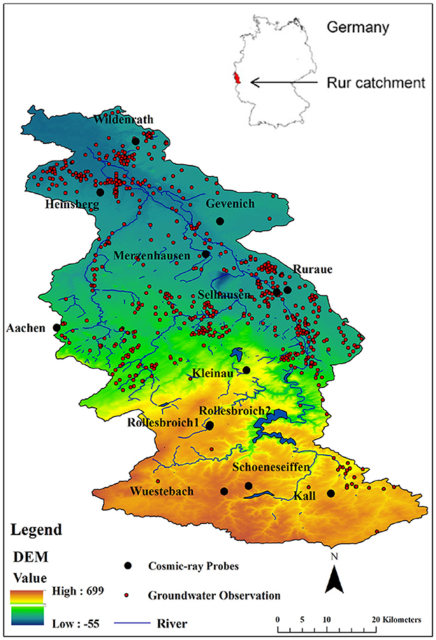
Figure 1. Map of the Rur catchment and locations of the 13 cosmic-ray neutron sensors (CRNS) (black points) and groundwater measurement sites (red points) in the year 2018. The Rur catchment is situated in western Germany.
The high-resolution (1:50,000) regional soil map BK50 (Nordrhein-Westfalen, 2009) (see Figure 2) and Pano (2006) were used to obtain the soil characteristics and to calculate the soil hydraulic properties. Bulk density was obtained from ESDB.
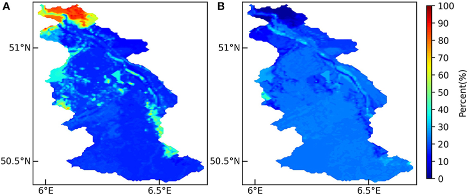
Figure 2. Sand (A) and clay (B) content (%) for the Rur catchment derived from the BK50 soil map.
Based on the thickness of the BK50 soil layers, we treat the layers below the soil layers as aquifer layers. The upper aquifer hydraulic conductivity (see Figure 3) was obtained from the Information System Hydrogeological Map of North Rhine-Westphalia with a resolution of 1:100,000 (https://www.opengeodata.nrw.de/produkte/geologie/geologie/HK/ISHK100/). The permeability of the aquifer is based on different classes of rock types.
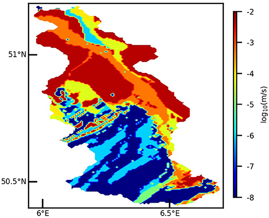
Figure 3. Hydraulic conductivity of the aquifer material for the Rur catchment.
The high-resolution reanalysis dataset COSMO-REA6 developed with the numerical weather prediction (NWP) model COSMO (Baldauf et al., 2011) is used as atmospheric forcing in this work (Bollmeyer et al., 2015; Wahl et al., 2017). Currently, the reanalysis covers the period 1995–2019 at a high spatial resolution of 0.055° (6 km) and is continuously extended by the German Weather Service (Deutscher Wetterdienst; DWD). The forcing data include precipitation, air temperature, air pressure, wind velocity, specific humidity, incoming shortwave radiation, and incoming longwave radiation.
The measured WTD data from the monitoring network Geoportal NRW (www.geoportal.nrw) were used for assimilation and some as independent verification data for the model simulations. For the year 2018, there were 865 sites located in shallow and deep aquifers of the Rur catchment that monitored the WTD (see Figure 1), and most measurement sites are distributed along the river. The observation frequency varies for each site, and can be daily, weekly, or monthly. In 2018, there were 575 sites with WTD between 0 and 20 m. We only used the sites with WTD between 0 and 20 m to be sure that only measurements from the upper aquifer were included for assimilation or verification, as our model only considered the upper 20 m.
CRNS is a precise method to measure soil moisture at the field scale (Zreda et al., 2008; Baatz et al., 2014; Köhli et al., 2015). The Rur catchment CRNS network comprises 13 CRNS stations (see Table 1) (CRS1000, HydroInnova LLC, 2009) (Baatz R. et al., 2017; Bogena et al., 2022) and these observation sites are relatively evenly distributed over the study area (see Figure 1). CRNS measures the fast neutron intensity, and the measured number of neutron counts shows an inverse correlation with soil moisture content. Fast neutrons originate from the collisions of secondary cosmic particles from outer space with terrestrial atoms. Fast neutrons are moderated most effectively by hydrogen, since the mass of the neutron is similar to the mass of a nucleus of the hydrogen atom. Thus, the corresponding fast neutron intensity measured by CRNS strongly depends on the amount of hydrogen within the CRNS footprint, allowing for a continuous non-invasive soil moisture estimate at the field scale (Baatz R. et al., 2017). The horizontal footprint of this measurement matches the 500 m horizontal model resolution quite well. It can measure soil moisture until 83 cm depth under very dry conditions, and to 15 cm depth under very wet soil conditions (Köhli et al., 2015; Schrön et al., 2017).
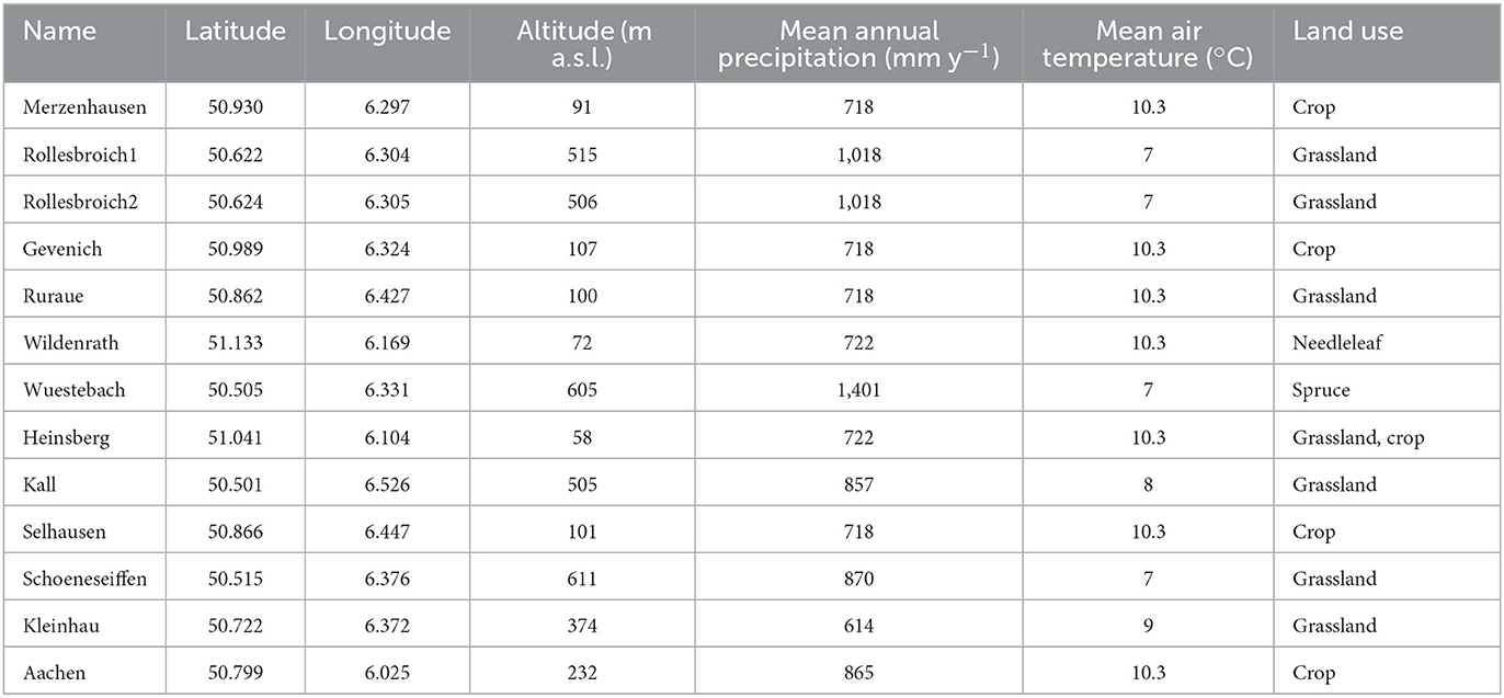
Table 1. CRNS sites with geographical information [from (Baatz R. et al., 2017; Bogena et al., 2022)].
2.2. Model description (TSMP)
The coupled terrestrial system model used consists of three compartments integrated under the framework TSMP, the 3D variably saturated groundwater flow model ParFlow for the subsurface (Kollet and Maxwell, 2006), the land surface model CLM version 3.5 (Community Land Model) from the National Center for Atmospheric Research (Oleson et al., 2007, 2008), and the numerical weather prediction model COSMO (Consortium for Small Scale Modeling) (Baldauf et al., 2011). These three models are two-way coupled by the Ocean Atmosphere Sea Ice Soil coupling Model Coupling Toolkit (OASIS-MCT, version 3) (Valcke, 2013). The integrated modeling platform TSMP can run with different combinations of the component models (Shrestha et al., 2014). In this study, CLM-ParFlow was used without COSMO.
2.2.1. Land surface model CLM
The biophysical processes simulated by CLM3.5 include solar and longwave radiation interactions with vegetation canopy and soil, momentum and turbulent fluxes from canopy and soil, canopy hydrology (e.g., interception processes), soil hydrology, and stomatal physiology and photosynthesis (Oleson et al., 2007). The mass and energy balance solved by CLM include soil evaporation, evaporation from intercepted water, transpiration from plants, infiltration of water in the soil, sensible and ground heat fluxes, and freeze-thaw processes (Oleson et al., 2007, 2008).
The nested subgrid hierarchy is used to represent spatial land surface heterogeneity (Oleson et al., 2008). Each grid cell is divided into a variety of land units (glacier, lake, wetland, urban, and vegetated), where each land unit can have a different number of snow/soil columns, and each column can have multiple plant functional types (PFTs) (Bonan et al., 2002; Oleson et al., 2008). In CLM, the soil column and snow column are discretized into 10 and 5 vertical layers, respectively (Oleson et al., 2007, 2008). Each PFT is characterized by distinct plant physiological parameters, which could capture the biogeophysical and biogeochemical differences between the different vegetation types (Oleson et al., 2007, 2008).
2.2.2. Subsurface hydrological model ParFlow
In TSMP, the soil hydrology of CLM is substituted by the soil hydrology of ParFlow (Kollet and Maxwell, 2008) and also surface runoff and groundwater flow are calculated by ParFlow. ParFlow is a three-dimensional variably saturated groundwater flow model improved with a two-dimensional overland flow simulator (Ashby and Falgout, 1996; Kollet and Maxwell, 2006). It combines the kinematic wave equation (Lighthill and Whitham, 1955) and the 3D Richards' equation (Richards, 1931) to describe the dynamic coupling of surface-subsurface flow under overland flow boundary conditions (Kollet and Maxwell, 2006). In ParFlow, the three-dimensional Richards' equation can be written as follows (Maxwell, 2013):
and,
where Ss is the specific storage [L−1]; Sw is the relative saturation; h is the pressure-head [L]; t is time [T]; Φ is the porosity; q is the specific volumetric (Darcy) flux [LT−1]; qr is a general source/sink term that represents transpiration, wells, and other fluxes [LT−1]; x is the length along the x-axis specified as horizontal direction [L]; z is the elevation along the z-axis specified as upward to be positive [L]; v is the subsurface flow velocity [LT−1]; Ks(x) is the saturated hydraulic conductivity tensor [LT−1]; kr is the relative permeability.
ParFlow requires input soil hydraulic parameters like saturated hydraulic conductivity, porosity, and Mualem-van Genuchten parameters (van Genuchten, 1980; Kollet and Maxwell, 2008). For our study, saturated hydraulic conductivities of soil layers were calculated from sand, silt and clay contents and bulk density using the software rosettav3 H3, which is based on an artificial neural network analysis coupled with a bootstrap resampling method (Schaap et al., 2001; Zhang and Schaap, 2017). To keep hydraulic consistency between CLM and ParFlow, porosity (θs) for both models is calculated on the basis of the sand fraction via the following pedotransfer function in CLM (Oleson et al., 2007):
The van Genuchten formulation (van Genuchten, 1980) is employed to evaluate the pressure head from soil moisture data:
where Ψ is subsurface pressure head [L]; θs is porosity; θr is residual soil moisture content; α is a measure of the first moment of the pore size density function [L−1]; n is an inverse measure of the second moment of the pore size density function; and m = 1-1/n.
The Newton Krylov solution technique is applied in ParFlow and acts as a non-linear solver (Jones and Woodward, 2001). The coupled partial differential equations for subsurface flow and surface water flow are solved by the Newton-Krylov method with multigrid preconditioning, which is good at handling subsurface flow problems at large-scales in highly heterogeneous media and under variably saturated conditions (Kollet and Maxwell, 2006, 2008; Maxwell, 2013). A prominent advantage of ParFlow is that it was designed for parallel computer systems, so that it can efficiently compute large-scale problems at high resolution, which has been demonstrated in many studies (Jones and Woodward, 2001; Kollet and Maxwell, 2006, 2008).
2.2.3. Coupling interface OASIS-MCT
The external coupler OASIS-MCT (Valcke, 2013) is used to couple CLM and ParFlow, and control the exchange of fluxes between the different component models (Shrestha et al., 2014). When the fluxes correspond to different spatial and temporal scales, OASIS-MCT uses time integration/averaging and spatial interpolation operators to keep the scales consistent (Sulis et al., 2015). In TSMP, ParFlow provides CLM with the upper 10 subsurface layers pressure and saturation, and in turn, CLM provides ParFlow with the upper boundary condition, which is net infiltration or exfiltration. The net infiltration includes precipitation, interception, total evaporation, and total transpiration (Zhang et al., 2018).
2.3. LEnKF methodology
DA consists of a forecast and an analysis step. For the forecast step, the state estimation is only based on past data (McLaughlin, 2002). For the analysis step, the information from current measurements and from a prior short-term forecast (which is based on past data) is used to produce a current state estimate. Then, the estimate will be used to initialize the next short-term forecast, which is subsequently used in the next analysis, and so on (Hunt et al., 2007). The EnKF sequentially performs a model forecast and a filter analysis. The efficiency of the filter relies on the accurate determination of the forecast error covariance from the ensemble, and the main sources of forecast errors are initial conditions, forcing data, model parameters, and model equations (Turner et al., 2008). Perturbation approaches can take these error sources for the ensemble generation into account.
For each ensemble member j at time step i, the state vector xj,i in the forecast step is updated by observations and model predictions and is given by:
where j is the ensemble member, xj,i is the model forecast state vector at time step i (pressure head in our study), M is the model TSMP, xj,i−1 is the earlier model analysis with state vector at time step i-1, qj,i is the vector with (perturbed) model forcings (perturbed forcings are precipitation, incoming shortwave radiation, incoming longwave radiation, and air temperature in this study) and pj,i denotes the model perturbation vector with parameters (porosity and saturated hydraulic conductivity in this study). In summary, in this work, the ensemble of model realizations is generated by different initial conditions, forcings, and parameters. Model forecasts are updated according to:
Where, yj,i is the vector with (perturbed) observations, and the superscripts a and f refer to the updated state vector (the analysis) and the model predicted state vector, respectively. The observation operator Hi is used to map model forecasts into the observation space, which is here assumed to be linear, and Ki denotes the Kalman gain that is calculated as:
where Ri is the measurement error covariance matrix, and Pi is the model covariance matrix, which is calculated from the forecasted ensemble of model simulations at time step i according to:
where is a vector with ensemble mean values for the model states at time step i. N is the number of ensemble members.
The estimation of the covariances with a limited ensemble is affected by strong sampling fluctuations, and the estimated covariances might be affected by spurious correlations (Houtekamer and Mitchell, 1998, 2001). Houtekamer and Mitchell (1998) suggested a localization approach to remove spurious correlations to avoid filter divergence, limiting the updates to the surroundings of observations. Based on the localization of the error covariances proposed by Houtekamer and Mitchell (2001), in the evaluation of the Kalman gain in Equation 7, Pi is replaced by ρ°Pi, ρ°Pi represents the Schur product of the correlation matrix ρ and covariance matrix Pi, where ρ is a correlation matrix containing correlations between the grid cells (which are set to zero for grid cell combinations that are separated beyond a certain threshold). And the ρ and Pi should have the same dimensions, so the LEnKF analysis scheme can be expressed as:
Here ρ is determined by using a fifth-order piecewise function, as given by Gaspari and Cohn (1999). The correlation ω between a grid point and an observation, i.e., an element in ρ, can be approximated as Hu et al. (2012):
Where, l is the defined localization radius and e is the Euclidean distance between an analyzed grid point and an observation location. The correlations ω are distance-dependent and vary between 1 at observation locations and 0 at distances greater than twice the influence radius l. Only the observations located within the localization radius from an analyzed grid point can contribute to the analysis for this grid point (Hu et al., 2012). The cutoff radius can filter out small and noisy correlations associated with remote observations (Houtekamer and Mitchell, 2001). A larger radius may contain more spurious correlation, resulting in less effective assimilation. In contrast, a radius that is too small limits the influence of observations too much to update neighboring grid cells. Therefore, determining an appropriate assimilation localization radius is crucial.
2.4. Assimilation methodology
To be able to assimilate WTD measurements into TSMP, WTD data need to be transferred into pressure accordingly (see Figure 4). At locations with WTD measurements, the pressure head in the saturated zone is calculated from the measured WTD assuming a hydrostatic pressure distribution, according to Zhang et al. (2018):
Where Ψi is the pressure head at the ith soil layer [L], Di is the depth from land surface to the ith soil layer [L], and WTDobs is the observed WTD [L].
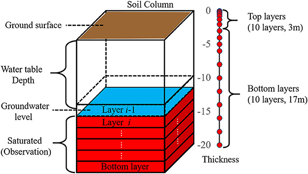
Figure 4. Illustration of the link between groundwater level observation and data to be assimilated [revised from Zhang et al. (2018)]. The blue color indicates the groundwater level at layer i-1. The red layers (from layer i to the bottom layer) are saturated and are incorporated as groundwater observations, and converted to pressure heads assuming hydrostatic conditions.
In our study, in order to ensure stability and avoid the occurrence of anomalous pressure values in the unsaturated zone related to updating pressure in the DA step, a weakly coupled approach was followed, which implies that only pressure in saturated layers is updated during assimilation. Hung et al. (2022) found that the weakly coupled approach outperformed the fully coupled approach for assimilating WTD measurements in TSMP. In the OL run, the vertical division between the unsaturated and saturated zones will differ among ensemble members. But as stated in Zhang et al. (2018), every grid cell should be updated consistently in DA, so the definition of the state vector should be the same for all ensemble members. The saturated and unsaturated zones are defined by the deepest WTD among the ensemble members, following Zhang et al. (2018). In the analysis step, only the pressure head values for the defined saturated zone will be directly updated via LEnKF.
3. Experimental setup
3.1. Ensemble generation and simulations
The simulation domain was discretized with a horizontal spatial resolution of 500 m. The study domain has a vertical extension of 20 m, which is discretized into 20 soil and aquifer layers with variable thicknesses. The thicknesses of the 10 uppermost layers increase exponentially with depth and extend to a total of 3 m. The deeper ten subsurface layers have thicknesses of 1 m (three layers) or 2 m (seven layers).
It is expected that the assimilation performance improves with increasing ensemble size (number of realizations), as found, for example, in studies with groundwater flow models (Chen and Zhang, 2006). An increasing ensemble size also implies higher computational costs. Hendricks Franssen and Kinzelbach (2008) indicated that 100 realizations should be sufficient for real-time groundwater flow modeling problems with state updating only. For combining state and parameter estimation, the ensemble size needs to be larger. As a compromise between accuracy and available compute time and data storage, we established an ensemble with 128 members for WTD assimilation in this work.
Meteorological forcings, hydraulic conductivities, and porosity were perturbed to generate the ensemble. Four atmospheric variables were perturbed: precipitation, incoming shortwave radiation, incoming longwave radiation, and air temperature. The meteorological forcings were perturbed without spatial correlation, while temporal correlations were induced by a first-order autoregressive model (Reichle et al., 2010; Han et al., 2015). Since the four meteorological variables are correlated, random values were drawn from a multivariate normal distribution. The statistics of the perturbed atmospheric variables are summarized in Table 2. The temporal correlations and standard deviations of the perturbations were chosen based on previous catchment-scale and regional-scale DA experiments (Reichle et al., 2010; Han et al., 2013, 2015; Baatz R. et al., 2017).
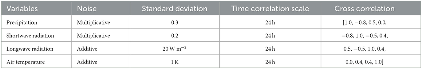
Table 2. The listed cross-correlations give the cross-correlations between the perturbations for the different atmospheric variables, following the order as indicated in the left column of the table.
Precipitation and shortwave radiation were multiplied by lognormally distributed noise (Han et al., 2013). A direct back transformation would induce a bias (resulting typically in a larger mean precipitation and larger mean incoming shortwave radiation), and therefore a correction is applied (Yamamoto, 2007):
Where, is the bias corrected perturbed variable of ensemble member j at day i, Zi is the original variable at day i, K is the corrective factor, and xj,i is the random perturbation of ensemble member j at day i from the multivariate normal distribution. N is the number of ensemble members (128 in this study).
Not only atmospheric forcing, but also hydraulic conductivity was perturbed in this study as the uncertainty of this parameter is in general large with an important effect on the groundwater flow prediction. We use different Ks data for the upper soil layers and lower aquifer layers. Hence, the Ks values of the soil and aquifer layers were perturbed separately (Table 3). The Ks values for soil layers were perturbed by perturbing the sand and clay contents first, and then applying the Rosetta pedotransfer functions (Schaap et al., 2001; Zhang and Schaap, 2017) to obtain the perturbed Ks. Sand and clay content were perturbed by calculating a field of spatially correlated perturbation values with geostatistical simulation and mean zero. A spherical variogram model was used, with nugget 0, sill of 50%2, and range 25 km. In order to avoid unphysical values for the soil textures, the sum of the sand and clay content were constrained between 0 and 100%. The Ks of the bottom aquifer layers were perturbed for each hydrogeological unit by taking a value from a univariate uniform distribution with values between −0.5 and −0.5 and adding this to the mean Ks of the unit [log10(m/s)]. The porosity for the upper soil layers was determined according to Equation 3 and on the basis of the perturbed sand contents, while for the bottom aquifer layers, the constant value of 0.15 was used, without perturbation.
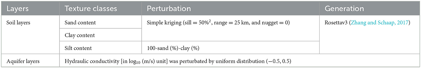
Table 3. Perturbation of saturated hydraulic conductivities for different subsurface layers.
It is known from previous studies that the spin-up for the model TSMP significantly influences the simulated WTD. The 100 year spin-up for 128 ensemble members departed from a WTD of 0 m, and was forced by 30-year average recharge values (derived from gridded data of precipitation and actual evapotranspiration provided by the German Weather Service) as an upper boundary condition. Next, an exit spin-up was done by running CLM-ParFlow for additional 10 years, using meteorological forcings from the year 2017 for all 10 years. The conditions at the end of the spin-up were used to initialize the DA experiments for the year 2018. The model time step is set to hourly.
3.2. Selection criteria for assimilated sites
There is a spatial mismatch between the point-scale groundwater measurements and the TSMP grid cell size of 500 m. In order to compare the measured WTD data with the model simulated values, each groundwater observation site was assigned to the nearest grid cell center. It is therefore common to have several measurement sites located in the same grid cell. We kept the groundwater measurement site which had the median value of all measurement sites in the grid cell for the year 2018, while the rest of the measurement sites were excluded from assimilation.
In addition, due to the relatively coarse model resolution, some measurement sites were located in model river grid cells. If all soil layers for each ensemble member in a grid cell were saturated for the complete year, the grid cell was considered to be a river grid cell. The river grid cells were eliminated from the analysis as groundwater measurements are not informative for the pressure values in river grid cells. Grid cells directly next to rivers were also excluded from the DA procedure, as these grid cells were also saturated most of the time and sometimes became part of the river. In this study, within the localization radius, we assimilated only observations from one site, with measurement values that are median values considering all sites in the localization radius.
In our study, the impact of the localization radius on the assimilation results was investigated, and three different localization radii were considered for assimilating groundwater measurements: 10, 5, and 2.5 km. According to the assimilation site selection criteria, three different localization radii resulted in 10 groundwater sites being selected for each of the DA experiments. Also, we used the groundwater data from unassimilated locations to investigate whether the localized assimilation could also improve the groundwater estimation at locations without assimilating data.
3.3. Evaluation of model performance
The root mean square error (RMSE) and bias (BIAS) were calculated to evaluate the performance of the WTD assimilation. The RMSE of WTD at each time step is calculated as:
where N is the total number of observation sites, is the ensemble average groundwater table depth of the grid cell where the observation site is located at the time step i (either from an OL run or a DA run), and is the observed WTD at the nth site and time step i.
The bias is also specified to quantify systematic differences between simulated and measured WTD:
In addition, simulation results were also compared with measured soil moisture content by CRNS. We follow the approach by Schrön et al. (2017), where weighted soil moisture content from the simulations was compared with CRNS measurements. The indicators, including BIAS, correlation coefficient (R), RMSE and unbiased root mean square difference (ubRMSD), are used to evaluate simulated soil moisture compared with the CRNS measurements. For each CRNS site, the above indicators were calculated individually and aggregated over time.
where T is the total number of time steps, is the simulated (either from an OL run or a DA run) ensemble average soil moisture content at the time step i, and is the observed soil moisture by CRNS at the time step i. The overbars in equations 16 and 18 indicate the temporal mean over the entire time period.
4. Results and discussion
4.1. Water table depth
4.1.1. Spatial autocorrelation analysis
For localized assimilation, the selection of the appropriate radius of localization is important. The localization radius should not be too small in order not to neglect positive correlations, and it should not be too long so that areas with spurious correlations are excluded. Therefore, we calculated the spatial autocorrelation of groundwater level measurements and simulated groundwater tables in the OL run (see Figure 5) to identify the appropriate radius. The spatial autocorrelations for different distance classes (0–0.5, 0.5–2.5, 2.5–5, 5–10, 10–20, 20–30, 30–40, 40–50, 50–60, and 60–70 km) were determined. The spatial correlation functions for the measured and WTD are quite close, implying that the model represents quite well the spatial correlation of the real groundwater levels in the Rur catchment. The largest differences are found for shorter distances, where the model autocorrelation is higher than the measured autocorrelation.
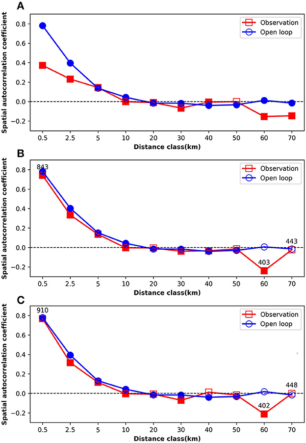
Figure 5. Spatial autocorrelation functions of measured and simulated (open loop) groundwater table depth for the year 2018 (A), the 26th of February 2018 (B), and the 24th of September 2018 (C). Filled squares or circles indicate autocorrelation coefficients are significantly different from zero (p < 0.05). When the number of comparison pairs was smaller than 1,000, the number of comparison pairs is indicated next to the marker.
4.1.2. Different localization radius assimilation strategies
Based on the spatial autocorrelation analysis, the localization radius could be up to 10 km. We tested 10, 5, and 2.5 km as localization radii, including 10 groundwater measurement sites for the assimilation.
For all scenarios, the RMSEs of WTD after 1 year of assimilation were lower than those of OL at the measurement locations (see Figure 6). The histogram of WTD errors at measurement locations also illustrates the improved WTD characterization after DA, compared with the OL. It can also be observed that the OL results on average in WTD values were larger than the measured ones, implying that the simulated WTDs were deeper than the measured ones. DA resulted in a reduction of the bias, and the peak of the histogram is closer to zero than OL. Thus, in all cases, LEnKF strongly reduced the bias and RMSE of WTD, compared to the scenario without assimilation of groundwater data, and the simulation improvement is best when using 10 or 5 km localization radius, and slightly worse for 2.5 km radius.
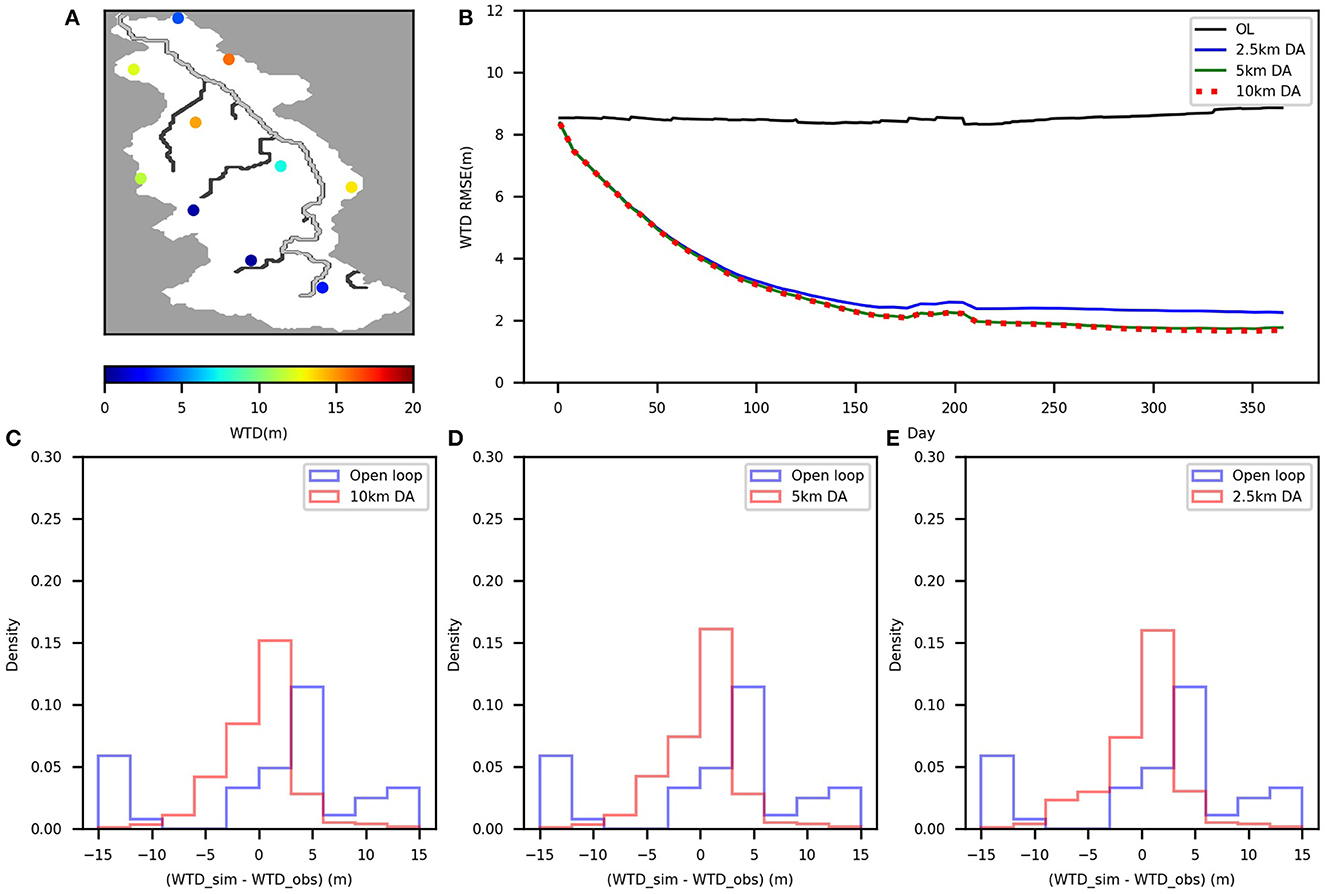
Figure 6. The locations of the assimilated groundwater sites (dots) in the Rur catchment together with the average groundwater table depth (A); time series of root mean square error (RMSE) of water table depth at measurement locations for the year 2018 for the open loop and data assimilation runs (B); the histogram of the water table depth errors at the measurement locations for the year 2018 from the open loop and data assimilation runs [10 km (C), 5 km (D), 2.5 km (E)].
Since the groundwater assimilation results for the three radii were similar at the assimilation sites, and the best results were obtained for the 10 km radius, only the simulated WTD from the 10 km localization radius DA run is shown in Figure 7, and compared with the WTD from the OL run and the measurements. The changes in groundwater levels during assimilation show that once assimilation starts, the WTD gets closer to the measurements.
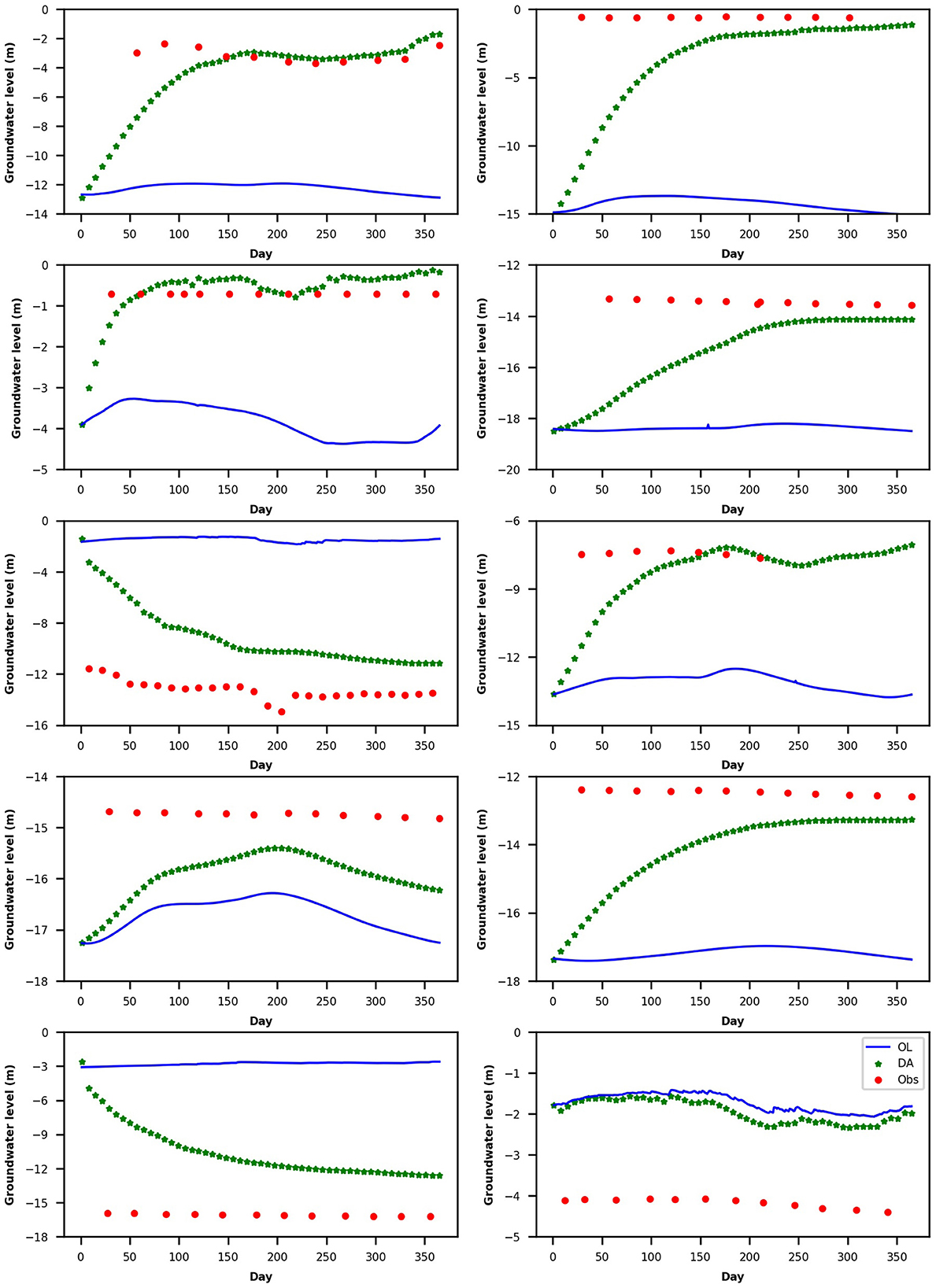
Figure 7. Water table depth time series for 10 assimilation sites: observations (Obs, red), ensemble mean of open loop (OL, blue) and ensemble mean of data assimilation run with 10 km localization radius (DA, green) for the year 2018.
The impact of the DA is similar for the different localization radii, with the same regions affected by increases or decreases in WTD (see in Figure 8). The main difference is that for a larger localization radius, the area updated by assimilation is larger, with a stronger reduction of ensemble standard deviations. However, for some areas, the ensemble standard deviation was larger for the DA run than for the OL run. This occurred when the measurements deviated strongly from the ensemble of OL runs. With DA, some ensemble members became closer to the observations, but others were not, resulting in an increase in the ensemble dispersion.
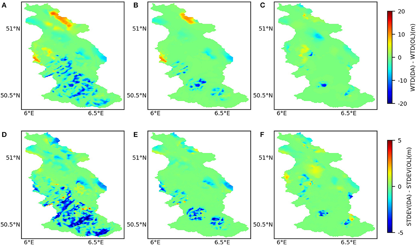
Figure 8. Difference in average water table depth between data assimilation and open loop runs (data assimilation–open loop) for different localization radii [10 km (A), 5 km (B), 2.5 km (C)] on the 31st of December 2018 for the Rur catchment; and difference in standard deviation for data assimilation and open loop runs for different localization radii [10 km (D), 5 km (E), 2.5 km (F)] on the 31st of December 2018 for the Rur catchment.
4.1.3. Data assimilation verification
To explore the impact of the assimilation of WTD measurements, we also evaluated the WTD characterization at verification locations (555 sites in total) which were not included in the assimilation, for the three different localization radii. We only show results for verification locations within the localization radius and only if enough measurement data were available for assimilation at a given time step (see Figure 9). Table 4 shows the RMSE for the OL and DA simulations, averaged for the period of 1year. At verification locations, the RMSE of the WTD also decreased, especially closer to the assimilation location, with verification locations separated <2.5 km from assimilation locations. DA could improve the groundwater simulation around measurement locations, which is consistent with the results by Hung et al. (2022).
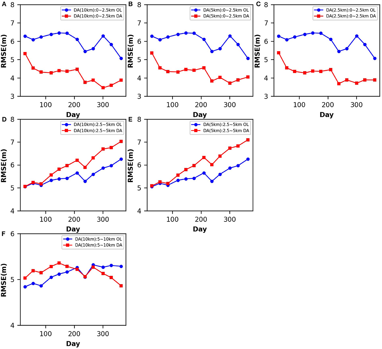
Figure 9. Time series of RMSE of groundwater table depth for the open loop (OL) and data assimilation (DA) runs [10 km (A, D, F), 5 km (B, E), 2.5 km (C) localization radius) at verification locations which were 0~2.5, 2.5~5, and 5~10 km away from assimilated observations.
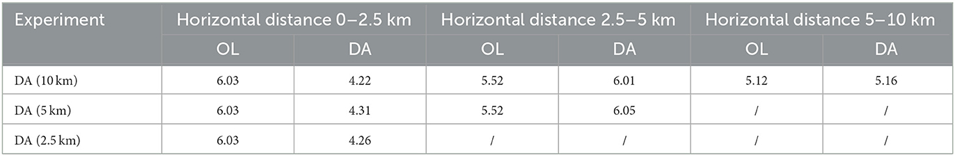
Table 4. The time averaged RMSE of the water table depth at the verification locations for the open loop (OL) and data assimilation (DA) runs (10 sites, 10, 5, and 2.5 km localization radius).
4.2. Soil moisture
The impact of WTD assimilation was also evaluated with in-situ soil moisture measurements from CRNS networks. Simulated soil moisture in OL and DA runs (for 10 and 5 km localization radius) was compared with CRNS measurements. The OL results indicate that simulated soil moisture contents have similar temporal variations as measured soil moisture contents (see Figure 10). Assimilation of WTD measurements did not result in an obvious improvement for soil moisture estimation (see Table 5). Hung et al. (2022) also found that assimilating groundwater table data only slightly improved soil moisture characterization with RMSE reductions between 1 and 6%, and the improvements were limited to a relatively small area around observation locations. This is related to the fact that soil moisture is only indirectly updated by the propagation of the pressure below the groundwater table. Therefore, when the groundwater table is deep, the impact of WTD assimilation on the upper soil moisture is small.
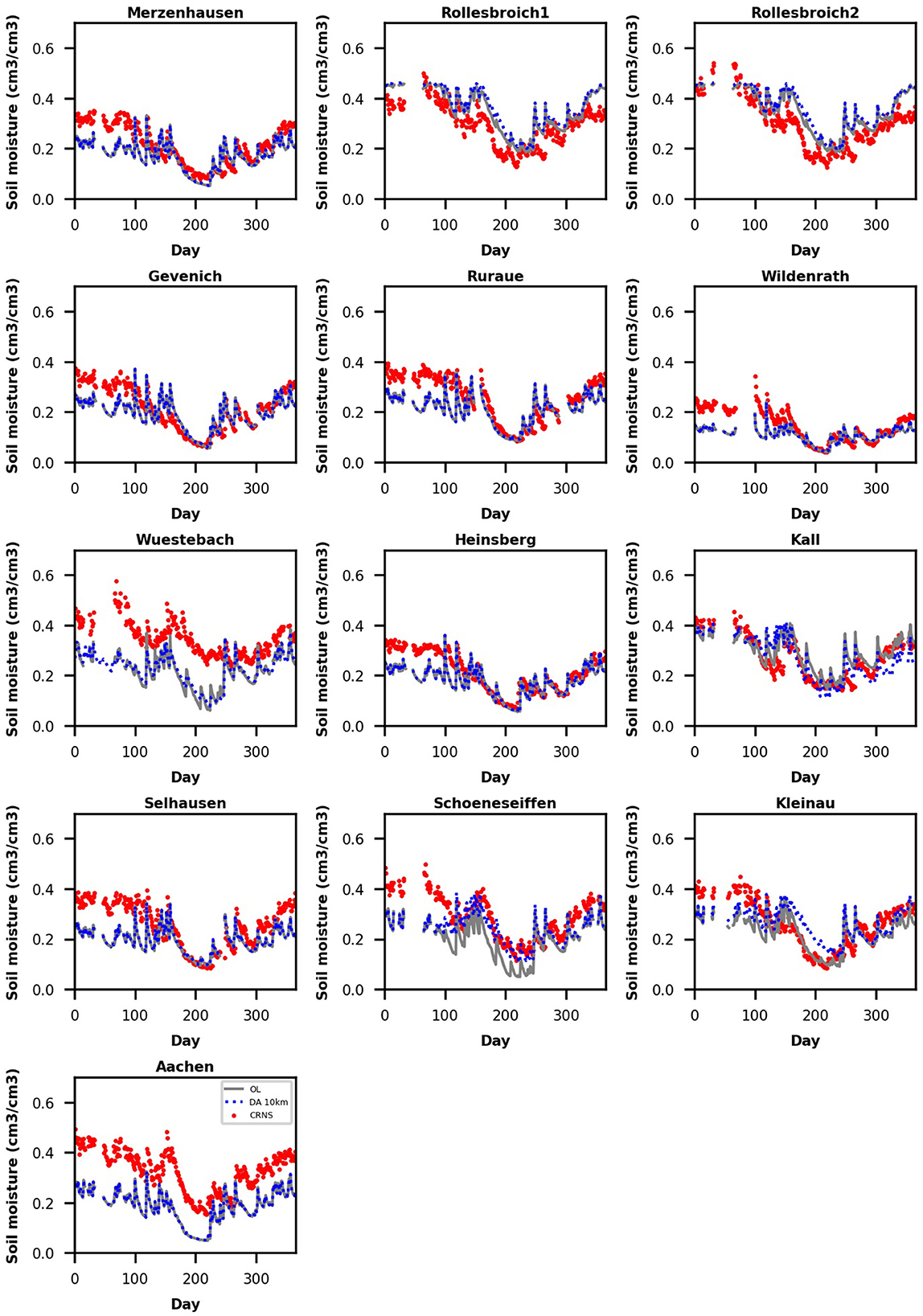
Figure 10. Soil moisture time series from cosmic-ray neutron sensors (CRNS) (red), ensemble mean of open loop (OL, gray), and ensemble mean of data assimilation with 10 km assimilation radius (DA 10 km, blue) for the year 2018.
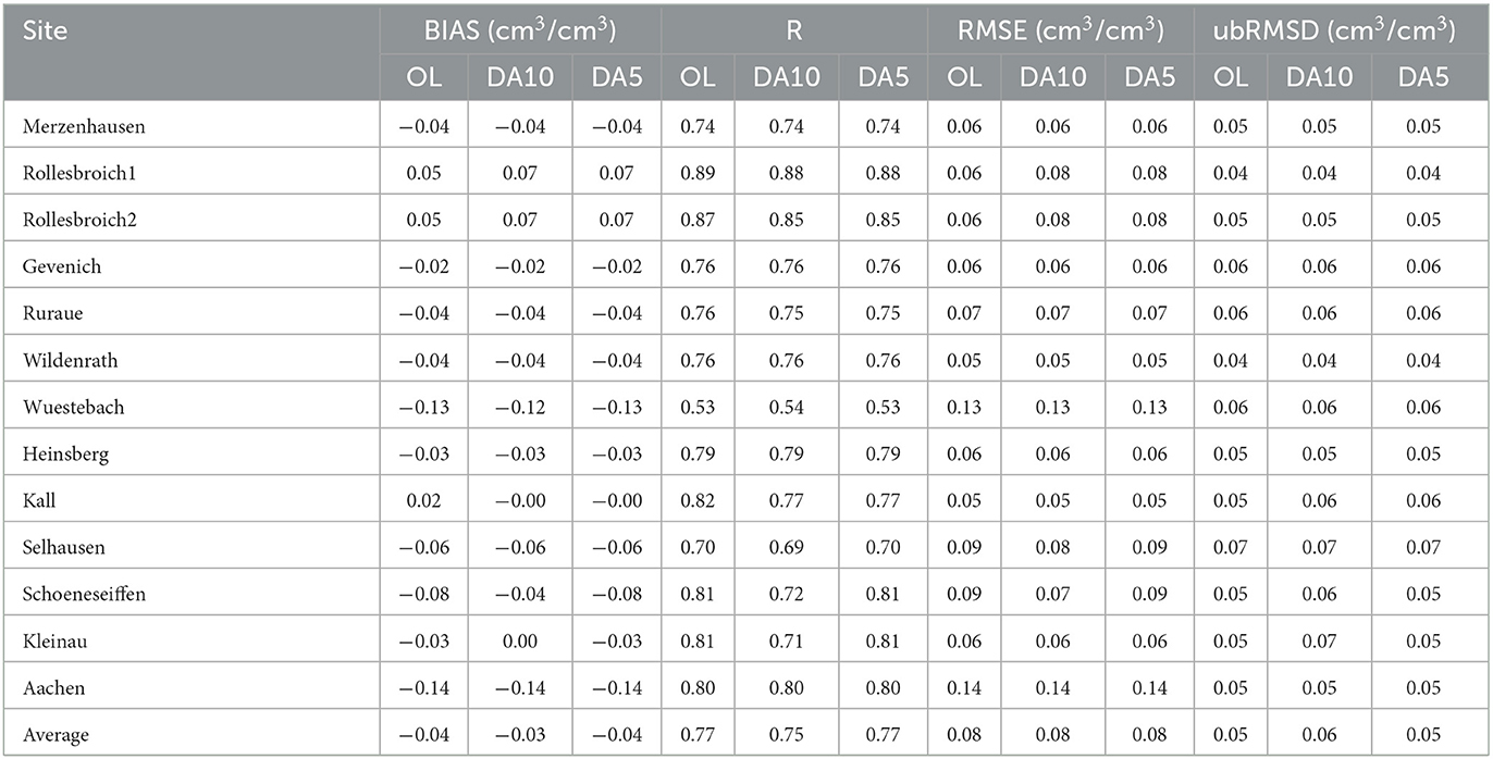
Table 5. Comparison metrics for the soil moisture from CRNS compared to open loop (OL) and data assimilation runs (DA10 and DA5 are for 10 and 5 km localization radius, respectively) for the year 2018.
4.3. Discussion
In all DA experiments, the estimation of the WTD improved, and also close to observation sites an improved groundwater characterization was found. This shows that for real-world cases, the localized EnKF could merge the integrated model TSMP with data to more accurately simulate the groundwater table.
There are some caveats regarding the use of in-situ groundwater observations to do assimilation and validate model estimates. Since the spatial representativeness of model and measurements are different, it is non-trivial to assimilate the in-situ groundwater measurements into the integrated model and to evaluate the coarse resolution model results against in-situ measurements. In our study, the model has a grid resolution of 500 m, while the groundwater measurements are obtained from points. Many observation sites were located in the same grid cell and were not included in the assimilation in this work. In future work, these measurements should be assimilated by modifying the measurement operator. However, this will not resolve all issues regarding scale mismatches. As the coarser model resolution flattens the topography, and therefore the gradients for surface and subsurface water flow, a systematic bias in the simulated groundwater table can be expected and is also observed in this study. In theory, for data assimilation, we should not have systematic differences between simulated and measured values, and prior bias correction would be a strategy to consider. In practice, we normally have to deal with systematic biases in data assimilation and if the ensemble spread is large enough, the model states can still be corrected toward the measurements. Removing the systematic bias in simulated groundwater levels with TSMP is not trivial as it depends on the model resolution. An extensive effort is needed to remove the systematic bias, which is a research question in itself and beyond the scope of this study. We argue that in the future better results can be obtained if a higher model resolution of 100 m instead of 500 m is used so that groundwater bodies related to narrow valleys can be better represented.
In addition, the model TSMP in this study only considers a vertical depth up to 20 m, and only one upper unconfined aquifer is better modeled. However, the real situation is much more complicated, as typically multiple unconfined and confined aquifer layers exist. As our model only models the 20 m subsurface, measurements relating to deeper aquifers were also excluded. In future work, an extension of the vertical depth could provide more realistic simulations, but for this, it would be important to have more detailed 3D geological information.
The spatial autocorrelation analysis indicates that groundwater levels were correlated for separation distances up to 10 km. However, groundwater level characterization was only improved in a smaller area for locations separated by <2.5 km from measurement sites. Hung et al. (2022) used a dense observation network in a synthetic experiment that closely mimicked the Neckar catchment of southwestern Germany, and proved that groundwater level assimilation could improve groundwater level estimation between the measurement locations. They found that the improvement of the groundwater level simulation decreased with increasing horizontal distance, and improvements in groundwater level simulations could extend to 8 km away from the observations for a localization radius of 12 km. Our results illustrate that for a real-world application, the improvement is more limited, which will be related to model structural errors like inadequate grid resolution and missing information on pumping activities.
Theoretically, only grid cells within the localization radius can be updated in the analysis step (Houtekamer and Mitchell, 2001). However, as the assimilation proceeds over time, updates around measurement locations can laterally propagate through the working of the physical equations, and this effect could be particularly strong in the saturated zone given the importance of lateral flow in the saturated zone. In the assimilation experiments with 10 and 5 km localization radius, there were no obvious improvements in the characterizations of soil moisture content by TSMP. Though the groundwater bias was corrected after assimilation, soil moisture does not change significantly with the change in deep groundwater tables. Also, Hung et al. (2022) discovered topography variations and lateral groundwater flow greatly influence groundwater levels, making soil moisture data probably less informative for groundwater levels, which also supports the findings of this study. Hung et al. (2022) found a slight improvement for soil moisture characterization related to groundwater level assimilation, which was not found in this study. The worse performance in this real-world study might be related to model structural errors, as Hung et al. (2022) simulated a catchment of similar complexity, but in a synthetic version that mimicked that catchment. A further reason might be the limited number of groundwater assimilation and soil moisture validation sites used in this study. We assimilated only groundwater level data, but soil moisture was not measured at the same locations, and soil moisture verification locations were separated from the groundwater monitoring sites.
Improved results can be expected for more ensemble members and/or a higher spatial resolution, which was not feasible in this work, as only one single DA experiment with 128 ensemble members required 73,728 core hours (the spin up not included) and 1.75 TB of computer storage for 1 year of simulation at a daily timescale.
Furthermore, although updating saturated hydraulic conductivities in Hung et al. (2022) only marginally improved the simulation of subsurface states, compared with only state updating, we will explore in future work the role of this important parameter in groundwater modeling. This should be evaluated for simulations at higher spatial resolution and larger ensemble sizes.
5. Conclusions
The localized Ensemble Kalman Filter was used to assimilate groundwater level measurements into the integrated terrestrial system model TSMP for the ~2,000 km2 Rur catchment. This is the first application of the assimilation of observed WTD data into the integrated land surface-subsurface model TSMP for a real-world case. Earlier work focused on a synthetic case, mimicking the Neckar catchment in southwest Germany. For the Rur catchment, 128 ensemble members were generated by perturbing four atmospheric forcing variables, saturated hydraulic conductivities and porosity. The perturbed ensemble was used as input in the TSMP-PDAF data assimilation framework and assimilation experiments were done for different localization radii (10, 5, and 2.5 km). The performance of WTD assimilation was assessed by comparing results from OL and DA experiments, and using groundwater observations and soil moisture measurements from cosmic ray neutron sensors as verification data. The main findings are:
1. The WTD simulated by the integrated model TSMP could be improved by localized EnKF, with more than 75% RMSE reduction at the assimilated locations for 3 different localization radii. The positive impact of assimilation is limited to the vicinity of the assimilated locations. The localized WTD assimilation is greatly affected by the unevenly distributed groundwater observations.
2. Simulated soil moisture generally reproduced the observed temporal fluctuations of soil water content, but soil moisture characterization was not improved after WTD assimilation. This can be related to the fact that only the saturated zone was directly updated via assimilation (and the unsaturated zone only indirectly), and the presence of model structural errors like a relatively coarse grid resolution of 500 m and missing information on groundwater pumping activities, for example.
3. Systematic differences between simulated and measured WTD might be related to the too coarse model resolution and model structural errors. Future work should focus on DA with integrated land surface-subsurface models at a higher spatial resolution and with more ensemble members, which would allow parameter estimation. In addition, the measurement operator needs to be considered for multiple groundwater level observations in a grid cell.
Data availability statement
The original contributions presented in the study are included in the article/supplementary material, further inquiries can be directed to the corresponding author.
Author contributions
FL and H-JHF designed the experiments. FL prepared the data for the experiments with the help from WK, conducted all the experiments and analyzed the results with feedback from CPH, HV, and H-JHF, and prepared the manuscript with contributions from all co-authors. All authors contributed to the article and approved the submitted version.
Funding
This research was funded by China Scholarship Council (CSC), grant number. 201904910448.
Acknowledgments
H-JHF gratefully acknowledges the supported by the project DETECT: Funded by the Deutsche Forschungsgemeinschaft (DFG, German Research Foundation)-SFB 1502/1-2022–Project number: 450058266. Furthermore, the authors gratefully acknowledge the computing time granted by the supercomputers JUWELS and JURECA at Forschungszentrum Jülich. We also thank the Terrestrial Environmental Observatories (TERENO) community to provide the data.
Conflict of interest
The authors declare that the research was conducted in the absence of any commercial or financial relationships that could be construed as a potential conflict of interest.
Publisher's note
All claims expressed in this article are solely those of the authors and do not necessarily represent those of their affiliated organizations, or those of the publisher, the editors and the reviewers. Any product that may be evaluated in this article, or claim that may be made by its manufacturer, is not guaranteed or endorsed by the publisher.
References
Ashby, S. F., and Falgout, R. D. (1996). A parallel multigrid preconditioned conjugate gradient algorithm for groundwater flow simulations. Nuc. Sci. Eng. 124, 145–159. doi: 10.13182/NSE96-A24230
Baatz, D., Kurtz, W., Hendricks Franssen, H. J., Vereecken, H., and Kollet, S. J. (2017). Catchment tomography - an approach for spatial parameter estimation. Adv. Water Resour. 107, 147–159. doi: 10.1016/j.advwatres.2017.06.006
Baatz, R., Bogena, H. R., Hendricks Franssen, H. J., Huisman, J. A., Qu, W., Montzka, C., et al. (2014). Calibration of a catchment scale cosmic-ray probe network: a comparison of three parameterization methods. J. Hydrol. 516, 231–244. doi: 10.1016/j.jhydrol.2014.02.026
Baatz, R., Hendricks Franssen, H.-J., Han, X., Hoar, T., Bogena, H. R., and Vereecken, H. (2017). Evaluation of a cosmic-ray neutron sensor network for improved land surface model prediction. Hydrol. Earth Syst. Sci. 21, 2509–2530. doi: 10.5194/hess-21-2509-2017
Baldauf, M., Seifert, A., Förstner, J., Majewski, D., Raschendorfer, M., and Reinhardt, T. (2011). Operational convective-scale numerical weather prediction with the COSMO model: description and sensitivities. Monthly Weather Rev. 139, 3887–3905. doi: 10.1175/MWR-D-10-05013.1
Bogena, H. R., Montzka, C., Huisman, J. A., Graf, A., Schmidt, M., Stockinger, M., et al. (2018). The TERENO-rur hydrological observatory: a multiscale multi-compartment research platform for the advancement of hydrological science. Vadose Zone J. 17, 180055. doi: 10.2136/vzj2018.03.0055
Bogena, H. R., Schrön, M., Jakobi, J., Ney, P., Zacharias, S., Andreasen, M., et al. (2022). COSMOS-Europe: a European network of cosmic-ray neutron soil moisture sensors. Earth Syst. Sci. Data. 14, 1125–1151. doi: 10.5194/essd-14-1125-2022
Bollmeyer, C., Keller, J. D., Ohlwein, C., Wahl, S., Crewell, S., Friederichs, P., et al. (2015). Towards a high-resolution regional reanalysis for the European CORDEX domain. Q. J. R. Meteorol. Soc. 141, 1–15. doi: 10.1002/qj.2486
Bonan, G. B., Levis, S., Kergoat, L., and Oleson, K. W. (2002). Landscapes as patches of plant functional types: an integrating concept for climate and ecosystem models. Global Biogeochem. Cycles. 16, 5-1–5-23. doi: 10.1029/2000GB001360
Camporese, M., Paniconi, C., Putti, M., and Salandin, P. (2009a). Ensemble Kalman filter data assimilation for a process-based catchment scale model of surface and subsurface flow. Water Resour. Res. 45, 1–14. doi: 10.1029/2008WR007031
Camporese, M., Paniconi, C., Putti, M., and Salandin, P. (2009b). Comparison of data assimilation techniques for a coupled model of surface and subsurface flow. Vadose Zone J. 8, 837–845. doi: 10.2136/vzj2009.0018
Chen, Y., and Zhang, D. (2006). Data assimilation for transient flow in geologic formations via ensemble Kalman filter. Adv. Water Resour. 29, 1107–1122. doi: 10.1016/j.advwatres.2005.09.007
Evensen, G. (1994). Sequential data assimilation with a nonlinear quasi-geostrophic model using Monte Carlo methods to forecast error statistics. J. Geophys. Res. 99, 143–110. doi: 10.1029/94JC00572
Evensen, G. (2003). The ensemble kalman filter: Theoretical formulation and practical implementation. Ocean Dynam. 53, 343–367. doi: 10.1007/s10236-003-0036-9
Freeze, R. A. (1975). A stochastic-conceptual analysis of the one-dimensional groundwater flow in nonuniform homogeneous media. Water Resour. Res. 11, 725–742. doi: 10.1029/WR011i005p00725
Furusho-Percot, C., Goergen, K., Hartick, C., Kulkarni, K., Keune, J., and Kollet, S. (2019). Pan-European groundwater to atmosphere terrestrial systems climatology from a physically consistent simulation. Sci Data. 6, 1–9. doi: 10.1038/s41597-019-0328-7
Gaspari, G., and Cohn, S. E. (1999). Construction of correlation functions in two and three dimensions. Q. J. R. Meteorol. Soc. 125, 723–757. doi: 10.1002/qj.49712555417
Gebler, S., Kurtz, W., Pauwels, V. R. N., Kollet, S. J., Vereecken, H., and Hendricks Franssen, H. J. (2019). Assimilation of high-resolution soil moisture data into an integrated terrestrial model for a small-scale head-water catchment. Water Resour. Res. 55, 10358–10385. doi: 10.1029/2018WR024658
Han, X., Franssen, H.-J. H., Montzka, C., and Vereecken, H. (2014). Soil moisture and soil properties estimation in the community land model with synthetic brightness temperature observations. Water Resour. Res. 50, 6081–6105. doi: 10.1002/2013WR014586
Han, X., Franssen, H. J. H., Rosolem, R., Jin, R., Li, X., and Vereecken, H. (2015). Correction of systematic model forcing bias of CLM using assimilation of cosmic-ray neutrons and land surface temperature: a study in the Heihe Catchment, China. Hydrol. Earth Syst. Sci. 19, 615–629. doi: 10.5194/hess-19-615-2015
Han, X., Hendricks Franssen, H.-J., Li, X., Zhang, Y., Montzka, C., and Vereecken, H. (2013). Joint assimilation of surface temperature and L-band microwave brightness temperature in land data assimilation. Vadose Zone J. 12, vzj2012.0072. doi: 10.2136/vzj2012.0072
Hendricks Franssen, H. J., and Kinzelbach, W. (2008). Real-time groundwater flow modeling with the ensemble kalman filter: joint estimation of states and parameters and the filter inbreeding problem. Water Resour. Res. 44, 1–22. doi: 10.1029/2007WR006505
Houtekamer, P. L., and Mitchell, H. L. (1998). Data assimilation using an ensemble kalman filter technique. Monthly Weather Rev. 126, 796–811. doi: 10.1175/1520-0493(1998)126<0796:DAUAEK>2.0.CO;2
Houtekamer, P. L., and Mitchell, H. L. (2001). A sequential ensemble kalman filter for atmospheric data assimilation. Monthly Weather Rev. 129, 123–137. doi: 10.1175/1520-0493(2001)129<0123:ASEKFF>2.0.CO;2
Hu, J., Fennel, K., Mattern, J. P., and Wilkin, J. (2012). Data assimilation with a local Ensemble Kalman Filter applied to a three-dimensional biological model of the middle atlantic bight. J. Marine Syst. 94, 145–156. doi: 10.1016/j.jmarsys.2011.11.016
Hung, C. P., Schalge, B., Baroni, G., Vereecken, H., and Hendricks Franssen, H. J. (2022). Assimilation of groundwater level and soil moisture data in an integrated land surface-subsurface model for Southwestern Germany. Water Resour. Res. 58, e2021WR031549. doi: 10.1029/2021WR031549
Hunt, B. R., Kostelich, E. J., and Szunyogh, I. (2007). Efficient data assimilation for spatiotemporal chaos: a local ensemble transform Kalman filter. Physica D 230, 112–126. doi: 10.1016/j.physd.2006.11.008
Jarvis, A., Guevara, E., Reuter, H. I., and Nelson, A. D. (2008). Hole-filled SRTM for the globe: version 4: data grid. Web publication/site. CGIAR Consortium for Spatial Information. Available online at: http://srtm.csi.cgiar.org/
Jones, J. E., and Woodward, C. S. (2001). Newton–Krylov-multigrid solvers for large-scale, highly heterogeneous, variably saturated flow problems. Adv. Water Resour. 24, 763–774. doi: 10.1016/S0309-1708(00)00075-0
Keune, J., Gasper, F., Goergen, K., Hense, A., Shrestha, P., Sulis, M., et al. (2016). Studying the influence of groundwater representations on land surface-atmosphere feedbacks during the European heat wave in 2003. J. Geophys. Res. Atmos. 121, 301–313. doi: 10.1002/2016JD025426
Köhli, M., Schron, M., Zreda, M., Schmidt, U., Dietrich, P., and Zacharias, S. (2015). Footprint characteristics revised for field-scale soil moisture monitoring with cosmic-ray neutrons. Water Resour. Res. 51, 5772–5790. doi: 10.1002/2015WR017169
Kollet, S. J., and Maxwell, R. M. (2006). Integrated surface–groundwater flow modeling: a free-surface overland flow boundary condition in a parallel groundwater flow model. Adv. Water Resour. 29, 945–958. doi: 10.1016/j.advwatres.2005.08.006
Kollet, S. J., and Maxwell, R. M. (2008). Capturing the influence of groundwater dynamics on land surface processes using an integrated, distributed watershed model. Water Resour. Res. 44, 1–18. doi: 10.1029/2007WR006004
Koster, R. D., Dirmeyer, P. A., Guo, Z., Bonan, G., Chan, E., Cox, P., et al. (2004). Regions of strong coupling between soil moisture and precipitation. Science 305, 1138–1140. doi: 10.1126/science.1100217
Kurtz, W., He, G., Kollet, S. J., Maxwell, R. M., Vereecken, H., and Hendricks Franssen, H.-J. (2016). TerrSysMP–PDAF (version 1.0): a modular high-performance data assimilation framework for an integrated land surface–subsurface model. Geosci. Model Develop. 9, 1341–1360. doi: 10.5194/gmd-9-1341-2016
Kurtz, W., Hendricks Franssen, H.-J., Kaiser, H.-P., and Vereecken, H. (2014). Joint assimilation of piezometric heads and groundwater temperatures for improved modeling of river-aquifer interactions. Water Resour. Res. 50, 1665–1688. doi: 10.1002/2013WR014823
Lighthill, M. J., and Whitham, G. B. (1955). “On kinematic waves I. Flood movement in long rivers,” in Proceedings of the Royal Society of London. Series A. Mathematical, Physical and Engineering Sciences (Royal Society), 281–316. doi: 10.1098/rspa.1955.0088
Maxwell, R. M. (2013). A terrain-following grid transform and preconditioner for parallel, large-scale, integrated hydrologic modeling. Adv. Water Resour. 53, 109–117. doi: 10.1016/j.advwatres.2012.10.001
McLaughlin, D. (2002). An integrated approach to hydrologic data assimilation: interpolation, smoothing, and filtering. Adv. Water Resour. 25, 1275–1286. doi: 10.1016/S0309-1708(02)00055-6
Montzka, C., Canty, M., Kunkel, R., Menz, G., Vereecken, H., and Wendland, F. (2008). Modelling the water balance of a mesoscale catchment basin using remotely sensed land cover data. J. Hydrol. 353, 322–334. doi: 10.1016/j.jhydrol.2008.02.018
Naz, B. S., Kollet, S., Franssen, H. H., Montzka, C., and Kurtz, W. (2020). A 3 km spatially and temporally consistent European daily soil moisture reanalysis from 2000 to 2015. Sci Data. 7, 11. doi: 10.1038/s41597-020-0450-6
Naz, B. S., Kurtz, W., Montzka, C., Sharples, W., Goergen, K., Keune, J., et al. (2019). Improving soil moisture and runoff simulations at 3 km over Europe using land surface data assimilation. Hydrol. Earth Syst. Sci. 23, 277–301. doi: 10.5194/hess-23-277-2019
Nerger, L., Hiller, W., and Oter, J. S. (2005). PDAF-the parallel data assimilation framework experiences with kalman filtering. Exp. Kalman Filt. 63–83. doi: 10.1142/9789812701831_0006
Nordrhein-Westfalen, G. D. (2009). Geologischer Dienst Nordrhein-Westfalen Informationssystem Bodenkarte 50. Available online at: https://www.opengeodata.nrw.de/produkte/geologie/boden/BK/ISBK50/
Oleson, K., Dai, Y., Bonan, G. B., Bosilovichm, M., Dickinson, R., Dirmeyer, P., et al. (2004). Technical Description of the Community Land Model (CLM) (No. NCAR/TN-461+STR). University Corporation for Atmospheric Research. doi: 10.5065/D6N877R0
Oleson, K. W., Niu, G. -Y., Yang, Z. -L., Lawrence, D. M., Thornton, P. E., Lawrence, P. J., et al. (2007). CLM3.5 documentation. National Center for Atmospheric Research, Boulder, CO, United States. p. 34.
Oleson, K. W., Niu, G. Y., Yang, Z. L., Lawrence, D. M., Thornton, P. E., Lawrence, P. J., et al. (2008). Improvements to the community land model and their impact on the hydrological cycle. J. Geophys. Res. Biogeosci. 113, 1–26. doi: 10.1029/2007JG000563
Pano, P. (2006). The European soil database, Vol. 5. p. 32–33. Available online at: https://esdac.jrc.ec.europa.eu/content/european-soil-database-v20-vector-and-attribute-data
Reichle, R. H., Crow, W. T., and Keppenne, C. L. (2008). An adaptive ensemble Kalman filter for soil moisture data assimilation. Water Resour. Res. 44, 1–13. doi: 10.1029/2007WR006357
Reichle, R. H., Kumar, S. V., Mahanama, S. P. P., Koster, R. D., and Liu, Q. (2010). Assimilation of satellite-derived skin temperature observations into land surface models. J. Hydrometeorol. 11, 1103–1122. doi: 10.1175/2010JHM1262.1
Reichle, R. H., McLaughlin, D. B., and Entekhabi, D. (2002). Hydrological data assimilation with the ensemble kalman filter. Monthly Weather Rev. 130, 103–114. doi: 10.1175/1520-0493(2002)130<0103:HDAWTE>2.0.CO;2
Richards, L. (1931). Capillary conduction of liquids through porous mediums. J. Appl. Phys. 318–333. doi: 10.1063/1.1745010
Schaap, M. G., Leij, F. J., and van Genuchten, M. T. (2001). Rosetta: a computer program for estimating soil hydraulic parameters with hierarchical pedotransfer functions. J. Hydrol. 251, 163–176. doi: 10.1016/S0022-1694(01)00466-8
Schrön, M., Köhli, M., Scheiffele, L., Iwema, J., Bogena, H. R., Lv, L., et al. (2017). Improving calibration and validation of cosmic-ray neutron sensors in the light of spatial sensitivity. Hydrol. Earth Syst. Sci. 21, 5009–5030. doi: 10.5194/hess-21-5009-2017
Shrestha, P., Sulis, M., Masbou, M., Kollet, S., and Simmer, C. (2014). A scale-consistent terrestrial systems modeling platform based on COSMO, CLM, and ParFlow. Monthly Weather Rev. 142, 3466–3483. doi: 10.1175/MWR-D-14-00029.1
Shrestha, P., Sulis, M., Simmer, C., and Kollet, S. (2015). Impacts of grid resolution on surface energy fluxes simulated with an integrated surface-groundwater flow model. Hydrol. Earth Syst. Sci. 19, 4317–4326. doi: 10.5194/hess-19-4317-2015
Sulis, M., Langensiepen, M., Shrestha, P., Schickling, A., Simmer, C., and Kollet, S. J. (2015). Evaluating the influence of plant-specific physiological parameterizations on the partitioning of land surface energy fluxes. J. Hydrometeorol. 16, 517–533. doi: 10.1175/JHM-D-14-0153.1
Turner, M., Walker, J., and Oke, P. (2008). Ensemble member generation for sequential data assimilation. Remote Sens. Environ. 112, 1421–1433. doi: 10.1016/j.rse.2007.02.042
UNWWAP (2015). Facts and Figures from the World Water Development Report. Document code: SC/2015/PI/H/2, SC-2015/WS/5 United Nations World Water Assessment Programme. Available online at: https://unesdoc.unesco.org/ark:/48223/pf0000231823
Valcke, S. (2013). The OASIS3 coupler: a European climate modelling community software. Geosci. Model Develop. 6, 373–388. doi: 10.5194/gmd-6-373-2013
van Genuchten, M. T. (1980). A closed-form equation for predicting the hydraulic conductivity of unsaturated soils. Soil Sci. Soc. Am. J. 44, 892–898. doi: 10.2136/sssaj1980.03615995004400050002x
Vereecken, H., Schnepf, A., Hopmans, J. W., Javaux, M., Or, D., Roose, T., et al. (2016). Modeling soil processes: review, key challenges, and new perspectives. Vadose Zone J. 15, 11–57. doi: 10.2136/vzj2015.09.0131
Wahl, S., Bollmeyer, C., Crewell, S., Figura, C., Friederichs, P., Hense, A., et al. (2017). A novel convective-scale regional reanalysis COSMO-REA2: improving the representation of precipitation. Meteorologische Zeitschrift. 26, 345–361. doi: 10.1127/metz/2017/0824
Waldhoff, G., and Lussem, U. (2015). Preliminary Land Use Classification of 2015 for the Rur Catchment. TR32DB [dataset], 10.5880/TR32DB.14. Available online at: https://www.tr32db.uni-koeln.de/data.php?dataID=1198
Yamamoto, J. K. (2007). On unbiased backtransform of lognormal kriging estimates. Comput. Geosci. 11, 219–234. doi: 10.1007/s10596-007-9046-x
Yu, H.-L., Wu, Y.-Z., and Cheung, S. Y. (2020). A data assimilation approach for groundwater parameter estimation under Bayesian maximum entropy framework. Stochastic Environ. Res. Risk Assess. 34, 709–721. doi: 10.1007/s00477-020-01795-z
Zhang, D., Madsen, H., Ridler, M. E., Kidmose, J., Jensen, K. H., and Refsgaard, J. C. (2016). Multivariate hydrological data assimilation of soil moisture and groundwater head. Hydrol. Earth Syst. Sci. 20, 4341–4357. doi: 10.5194/hess-20-4341-2016
Zhang, H., Kurtz, W., Kollet, S., Vereecken, H., and Franssen, H.-J. H. (2018). Comparison of different assimilation methodologies of groundwater levels to improve predictions of root zone soil moisture with an integrated terrestrial system model. Adv. Water Resour. 111, 224–238. doi: 10.1016/j.advwatres.2017.11.003
Zhang, Y., and Schaap, M. G. (2017). Weighted recalibration of the Rosetta pedotransfer model with improved estimates of hydraulic parameter distributions and summary statistics (Rosetta3). J. Hydrol. 547, 39–53. doi: 10.1016/j.jhydrol.2017.01.004
Keywords: groundwater, data assimilation, integrated model, real data, soil moisture, cosmic-ray neutron sensors
Citation: Li F, Kurtz W, Hung CP, Vereecken H and Hendricks Franssen H-J (2023) Water table depth assimilation in integrated terrestrial system models at the larger catchment scale. Front. Water 5:1150999. doi: 10.3389/frwa.2023.1150999
Received: 25 January 2023; Accepted: 28 February 2023;
Published: 22 March 2023.
Edited by:
Tongren Xu, Beijing Normal University, ChinaReviewed by:
Jianzhi Dong, Massachusetts Institute of Technology, United StatesDaniele Pedretti, University of Milan, Italy
Copyright © 2023 Li, Kurtz, Hung, Vereecken and Hendricks Franssen. This is an open-access article distributed under the terms of the Creative Commons Attribution License (CC BY). The use, distribution or reproduction in other forums is permitted, provided the original author(s) and the copyright owner(s) are credited and that the original publication in this journal is cited, in accordance with accepted academic practice. No use, distribution or reproduction is permitted which does not comply with these terms.
*Correspondence: Fang Li, Zi5saUBmei1qdWVsaWNoLmRl
†Present address: Wolfgang Kurtz, Department Agrometeorology, Deutscher Wetterdienst, Alte Akademie 16, Freising, Germany