High-resolution mapping of snow cover in montane meadows and forests using Planet imagery and machine learning

Yang, Kehan; John, Aji; Shean, David; Lundquist, Jessica D.; Sun, Ziheng; Yao, Fangfang; Todoran, Stefan; Cristea, Nicoleta

doi:10.3389/frwa.2023.1128758

ORIGINAL RESEARCH article

Front. Water, 01 June 2023

Sec. Water and Critical Zone

Volume 5 - 2023 | https://doi.org/10.3389/frwa.2023.1128758

This article is part of the Research Topic Advances in Observations and Modeling of Snow, Forest-Snow Processes and Snow Hydrology View all 5 articles

High-resolution mapping of snow cover in montane meadows and forests using Planet imagery and machine learning

$\r\nKehan Yang,$ Kehan Yang^1,2^*

Aji John^2,3

David Shean¹

Jessica D. Lundquist¹

Ziheng Sun⁴

Fangfang Yao⁵

Stefan Todoran⁶

Nicoleta Cristea^1,2

¹Department of Civil and Environmental Engineering, University of Washington, Seattle, WA, United States
²eScience Institute, University of Washington, Seattle, WA, United States
³Department of Biology, University of Washington, Seattle, WA, United States
⁴Center for Spatial Information Science and Systems, George Mason University, Fairfax, VA, United States
⁵Cooperative Institute for Research in Environmental Sciences, University of Colorado, Boulder, CO, United States
⁶Computer Science, University of Washington, Seattle, WA, United States

Mountain snowpack provides critical water resources for forest and meadow ecosystems that are experiencing rapid change due to global warming. An accurate characterization of snowpack heterogeneity in these ecosystems requires snow cover observations at high spatial resolutions, yet most existing snow cover datasets have a coarse resolution. To advance our observation capabilities of snow cover in meadows and forests, we developed a machine learning model to generate snow-covered area (SCA) maps from PlanetScope imagery at about 3-m spatial resolution. The model achieves a median F1 score of 0.75 for 103 cloud-free images across four different sites in the Western United States and Switzerland. It is more accurate (F1 score = 0.82) when forest areas are excluded from the evaluation. We further tested the model performance across 7,741 mountain meadows at the two study sites in the Sierra Nevada, California. It achieved a median F1 score of 0.83, with higher accuracy for larger and simpler geometry meadows than for smaller and more complexly shaped meadows. While mapping SCA in regions close to or under forest canopy is still challenging, the model can accurately identify SCA for relatively large forest gaps (i.e., 15m < DCE < 27m), with a median F1 score of 0.87 across the four study sites, and shows promising accuracy for areas very close (>10m) to forest edges. Our study highlights the potential of high-resolution satellite imagery for mapping mountain snow cover in forested areas and meadows, with implications for advancing ecohydrological research in a world expecting significant changes in snow.

1. Introduction

Seasonal snowpack covers about one-third of Earth's terrestrial surface at any time (Dozier, 1989), and its start, end, and duration impact the phenology of different types of vegetation and the functioning of snow-dominated ecosystems, such as montane meadows and forests (Dunne et al., 2003; Blankinship and Hart, 2012; Raleigh et al., 2013; Sherwood et al., 2017). However, traditional satellite observations are often unable to provide detailed information on the spatial distribution of snow cover in montane meadows and forest gaps due to their coarse spatial resolutions. Despite the availability of high-resolution satellite observations, few studies have explored the accuracy of snow cover mapping in montane forest gaps and meadows, where snowpacks exhibit high spatial heterogeneity.

Montane meadows are important ecosystems that have many critical functions, such as flood control, water quality improvement, and groundwater recharge (Loheide and Gorelick, 2007; Loheide and Lundquist, 2009). Meadows also provide unique wildlife habitats to animal and plant species, and recreation values for human beings (Hille Ris Lambers et al., 2021). Additionally, meadows are effective carbon sinks, and therefore, the restoration of meadows has a high potential to serve as climate change refugia to mitigate climate changes (Yang et al., 2019; Blackburn et al., 2021; Reed et al., 2022). Global warming has shifted the timing of snowmelt to earlier in the year and reduced snowpacks (Nijssen et al., 2001; Mote et al., 2018; Musselman et al., 2021), which could subsequently lead to changes in plant productivity and carbon sequestration over these seasonally snow-covered ecosystems (Vaganov et al., 1999; Brooks et al., 2005, 2011; Zona et al., 2022). Accurate mapping of seasonal snow cover in meadows is therefore important to understand the effects of changing snowpack on meadow ecosystems' functioning both now and in the future.

Accurate characterization of snow cover around forests and forest gaps is essential for effective natural resources management in montane forest ecosystems and for advancing the understanding of the critical interactions between forests and snow processes (Dickerson-Lange et al., 2015; Sun et al., 2018). Snow intercepted by the forest canopy sublimates more rapidly than snow on the ground, and therefore sublimation of snow intercepted by the forest canopy can lead to substantial reductions in snowpack volume over the course of a season. Meanwhile, forest canopy impacts the snowpack energy balance by emitting longwave radiation, shading insolation, and blocking wind. The net effect of these factors can result in a higher or lower snowmelt rate, with the direction and magnitude of the overall effect determined by climate factors as well as the type, density, and configuration of trees in the forest (Essery et al., 2008a,b; Pomeroy et al., 2008; Rutter et al., 2009; Lundquist et al., 2013; Musselman et al., 2015). However, due to the contradictory impacts, the duration of under-canopy snow cover could be longer or shorter than snowpack in the adjacent open areas, subject to local topography and climate conditions (Lundquist et al., 2013; Dickerson-Lange et al., 2015). Although observing under-canopy snow cover remains challenging, high-resolution optical satellite imagery provides new opportunities for mapping snow cover in forest gaps, which will advance our understanding of snow-forest interactions and will provide new insights to support forest and water resources management.

The use of remote sensing for SCA mapping has been evolving for more than five decades (Barnes and Bowley, 1968; Rango and Martinec, 1979; Dozier, 1984, 1989; Nolin et al., 1993; Hall et al., 2002; Painter et al., 2003, 2009; Dozier et al., 2008; Nolin, 2010; Gascoin et al., 2019; Rittger et al., 2020; Bair et al., 2021). One of the most popular methods for mapping SCA is the spectral index method, which uses the Normalized Difference Snow Index (NDSI). This method leverages the reflectance difference between the green and shortwave infrared bands to enhance the contrast between snow from non-snow land types on multispectral satellite imagery such as Landsat (Dozier, 1984, 1989), MODIS (Hall et al., 2010; Hall, 2012), and Sentinel-2 (Gascoin et al., 2019). While the NDSI thresholding method is simple and effective for classifying snow pixels, binary SCA maps generated from sensors with coarse resolution (e.g., 1.1 km for AVHRR, and ~500 m for MODIS) are often inadequate to accurately represent the variability of SCA across smaller scale features such as meadows and forest gaps.

Linear spectral mixture algorithms decompose mixed pixels and retrieve fractional snow-covered areas (fSCA). These algorithms assume that the reflectance of a pixel in a spectral band is a linear combination of weighted reflectance values of endmembers within the pixel (Nolin et al., 1993; Solberg and Andersen, 1994; Rosenthal and Dozier, 1996; Painter et al., 1998, 2003, 2009; Dozier and Painter, 2004; Bair et al., 2021). While spectral mixture algorithms have been shown to outperform the NDSI method in snow cover mapping and provide estimates of other important snow properties, such as snow grain size, snow albedo, and the impact of dust on snow albedo (Raleigh et al., 2013; Masson et al., 2018; Aalstad et al., 2020; Stillinger et al., 2022), they only provide fractional values of SCA for each pixel. When the spatial resolution of satellite data is coarse, these methods may not adequately capture the detailed spatial heterogeneity of SCA at a sub-pixel scale. Mapping and understanding fine-scale spatial heterogeneity of SCA are crucial for providing important insights into the impact of forest canopy on the snowpack.

Airborne lidar scanning also provides an effective means for observing snow cover at high spatial resolution (meter scale). This technique measures surface elevation once during snow-off conditions and repeatedly during snow-on conditions to derive snow depth, which is known to be reliable, even in forested areas (Currier and Lundquist, 2018; Mazzotti et al., 2019). Airborne lidar-derived snow depth data, such as the Airborne Snow Observatory snow depth dataset, thus have been widely used in previous studies to derive high-resolution SCA maps (Cristea et al., 2017; Raleigh and Small, 2017; Kostadinov et al., 2019; Cannistra et al., 2021; John et al., 2022; Stillinger et al., 2022), providing valuable insights into the spatial distribution of snow cover in complex mountain terrain.

In recent years, the commercial satellite industry has experienced rapid growth, with companies like Planet and Maxar providing new opportunities for Earth surface observations at sub-meter to meter-scale resolution, including snow identification in complex terrain (Cannistra et al., 2021; Hu and Shean, 2022). For example, Planet operates small satellite constellations that provide near-daily coverage of the Earth's land surface at about 3–5-m spatial resolution, making it an appealing data choice for investigations of snow patterns in mountainous regions. Previous studies have used convolutional neural networks (CNN) to map SCA from Planet PlanetScope images and achieved more accurate SCA maps than using traditional Landsat-8 and Sentinel-2 imagery for both forests and open areas (Cannistra et al., 2021; John et al., 2022). However, training CNN-based models is a time-consuming and potentially inefficient process given that it requires large training datasets and significant computational resources involving the use of graphics processing units (GPUs) and complex environment configurations. Therefore, there is a need for more efficient and less computationally demanding methods to map snow from high-resolution PlanetScope images.

In this study, we leverage PlanetScope imagery and a machine learning model to map high-resolution SCA and explicitly evaluate SCA accuracy in montane meadows and forest gaps. We chose to use a robust Random Forest model approach, which has been successfully applied to derive snow cover from many satellite images, such as MODIS (Liu et al., 2020; Kuter, 2021; Luo et al., 2022), Landsat-8 (Gascoin et al., 2019), Sentinel-1 SAR data (Tsai et al., 2019), Sentinel-2 (Gascoin et al., 2019), and high-resolution Maxar WorldView imagery (Hu and Shean, 2022). Additionally, Random Forest has shown good performance in data fusion approaches for mapping SCA (Rittger et al., 2021; Richiardi et al., 2023).

Following the introduction, Section 2 describes the study area and datasets, and Section 3 describes the SCA mapping model training and evaluation. The results and discussions are presented in Sections 4 and 5, respectively, with the summary and conclusion given in Section 6.

2. Study area and datasets

2.1. Study area

We selected three sites in the Western United States and one in Switzerland, covering a range of elevations, forest covers, meadow sizes, and availability of high-resolution validation data from Airborne Snow Observatory (ASO) lidar observations (details in Section 2.2.2). The four sites are (1) Tuolumne River Basin in the Central Sierra Nevada of California, (2) San Joaquin Main Fork in the Southern Sierra Nevada of California, (3) Gunnison—East River in the Central Rocky Mountains of Colorado, and (4) Engadin valley in the Eastern Swiss Alps of Switzerland (Figure 1). Hereafter, we refer to these sites only by the bold portion.

FIGURE 1

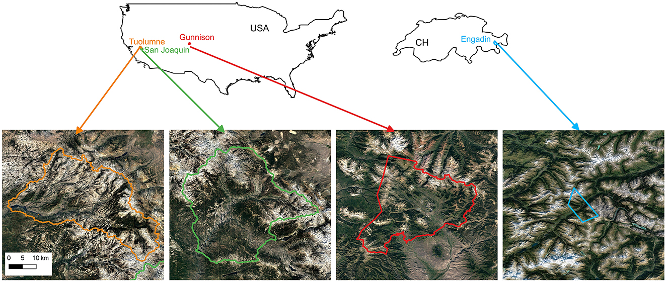
Figure 1. Context maps and satellite image base maps for the four study sites.

Among the four sites, Tuolumne and San Joaquin are in maritime mountain regions, while Gunnison and Engadin are in continental mountain regions. The San Joaquin site is the largest in size, with the highest forest coverage (50%) and the highest average canopy height (4.5 m). On the other hand, the Engadin site is the smallest, with the lowest forest coverage (22%) and second-shortest average canopy height (2.7 m; Table 1). The Gunnison site has the highest average elevation and the second-highest average canopy height (4.1 m), whereas the Tuolumne site has the lowest average canopy height (2.3 m; Table 1). The mean slopes of Tuolumne, San Joaquin, and Gunnison are similar, ranging from 20.2° to 22.7°, while the Engadin site has a higher mean slope of 34.4° due to the relatively smaller area being included in the study.

TABLE 1

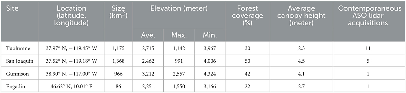
Table 1. Topographic characteristics of the four study sites and contemporaneous ASO lidar snow depth acquisitions that were used in the study.

2.2. Datasets

2.2.1. Planet CubeSat images

We used images from the PlanetScope constellation, which includes three generations of satellites: Dove Classic (PS2), Dove-R (PS2.SD), and SuperDove (PSB.SD; Figure 2). To map SCA, we used an atmospherically corrected surface reflectance product (Level-3B Ortho Scene-Analytic) that underwent rigorous geometric and radiometric correction techniques, orthorectified, and passed all image quality checks in the Planet processing pipeline (Frazier and Hemingway, 2021).

FIGURE 2

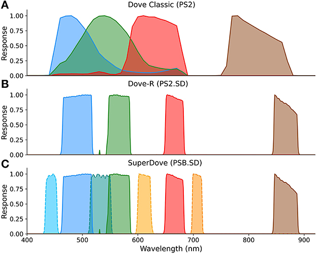
Figure 2. The distribution of spectral response in three generations of PlanetScope satellites (adapted from Frazier and Hemingway, 2021), (A) Dove Classic (PS2), (B) Dove-R (PS2.SD), and (C) SuperDove (PSB.SD). The blue, green, red, and brown curves correspond to the spectral response of blue, green, red, and near-infrared bands, respectively. For the SuperDove instrument, which has eight bands, we used dashed lines to represent the extra four bands that are not used in the model. The earliest imagery from PS2, PS2.SD, and PSB.SD was acquired in July 2014, March 2019, and March 2020, respectively.

PlanetScope images provide at least four bands, including three visible bands (red, green, and blue) and one near-infrared band (Figure 2). Although the wavelength ranges of these bands are similar among the three Dove generations, they are not identical due to changes in sensors over time. The first-generation Dove Classic sensors lack spectral response separation in RGB bands, while Dove-R and SuperDove have comparable widths and placements of four bands (RGB and near-infrared). SuperDove also provides four additional bands in the visible portion of the spectrum (Figure 2). While including reflectance information from additional SuperDove bands may add value to snow cover mapping, the four bands we excluded do not extend the range of the RGB wavelength where snow reflectance is typically high, nor do they process any distinctive features. To ensure that our method would apply to all PlanetScope images, regardless of Dove generation, we chose not to include the extra SuperDove bands for snow cover mapping in this study.

However, none of the PlanetScope spectral bands, including the four additional excluded bands from SuperDove, cover the shortwave infrared (SWIR) portion of the electromagnetic spectrum that is used for the calculation of NDSI and plays an important role in the spectral unmixing models. The lack of SWIR band in the PlanetScope images is the main reason why the more traditional SCA mapping methods such as NDSI or spectral unmixing models which have been used across a range of sensors with only minor changes are not easily adapted to work with PlanetScope images (Cannistra et al., 2021). Additionally, snow and clouds exhibit similar spectrum features and high reflectance in the visible and NIR bands, making it challenging to distinguish between snow and clouds.

Therefore, we screened out PlanetScope images with cloud cover higher than 5% based on the “cloud coverage” metadata provided by Planet. Considering the uncertainty in cloud coverage and image issues like saturation, we further reviewed and manually excluded 11 images, for a total of 103 PlanetScope images finally used in this study.

2.2.2. ASO Snow depth and canopy height model

Airborne Snow Observatory (ASO), Inc is a commercial company that provides airborne snow depth and snow water equivalent (SWE) at very high spatial resolutions (i.e., 3-m for snow depth and 50-m for SWE). The snow depth product has an 8 cm root mean squared error at 3-m spatial resolution when evaluated with 80 ground observations over a relatively flat area near Tioga Pass, California (Painter et al., 2016). While more comprehensive evaluation is needed, the ASO snow depth data are accepted as the current standard by the community and have increasingly been used to create high-resolution SCA maps, which have been used as independent ground “truth” validation data (Cristea et al., 2017; Kostadinov et al., 2019; Cannistra et al., 2021; John et al., 2022; Stillinger et al., 2022). Therefore, in this study, we used the SCA maps derived from ASO snow depth data as ground reference to evaluate SCA mapped from PlanetScope images.

We identified and processed PlanetScope images acquired on the same days as ASO lidar acquisitions at the four study sites (Table 1). Since the Tuolumne site has the longest record of lidar collections and the most frequent observations, we processed all contemporaneous PlanetScope images for the Tuolumne site from 2017 to 2022 to cover various snow conditions. We excluded dates with relatively low coverage of contemporaneous cloud-free PlanetScope images and ASO snow depth data. In total, we processed 18 ASO snow depth acquisitions for the four sites (Table 1). The 3-meter snow depth data for the years between 2017 and 2019 were downloaded from the National Snow and Ice Data Center (Painter, 2018), while the snow depth data after 2019 were downloaded from the ASO, Inc. website (https://data.airbornesnowobservatories.com).

We utilized the canopy height model data (CHM) provided by the ASO team to determine the extent of forests in the four study sites (details provided in Section 3.3). The CHM data for Tuolumne, San Joaquin, Gunnison, and Engadin were collected on 27 August 2014, 23 October 2016, 8 September 2018, and 29 August 2017, respectively (Currier and Lundquist, 2018; Mazzotti et al., 2019).

2.2.3. Meadow extent

The Sierra Nevada Multi-source Meadow Polygons Compilation Version 2 (SNMMPC v.2, Weixelman et al., 2011; UC Davis, 2017) was used to delineate meadow extent for two study sites: Tuolumne and San Joaquin. As meadow data were not available for Gunnison and Engadin, these two sites were excluded from the model accuracy assessment for meadow areas. The SNMMPC v.2 dataset was created by the University of California, Davis, and the United States Department of Agriculture Forest Service and comprises all meadows larger than one acre (4,047 m²), providing the most comprehensive spatial data on mountain meadows for the Sierra Nevada, California. The dataset can be downloaded from https://meadows.sf.ucdavis.edu/resources/326.

3. Method

The workflow of SCA mapping using PlanetScope imagery includes three main steps (Figure 3). In brief, we first downloaded and visually checked PlanetScope images. Then we trained the SCA mapping model following the steps illustrated in Figure 3 (details in Section 3.2); the last step was SCA evaluation (details in Section 3.3).

FIGURE 3

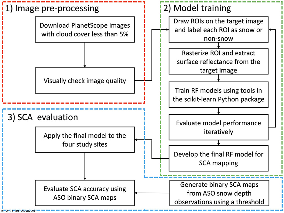
Figure 3. Flowchart of the model developed to map snow-covered area (SCA) using PlanetScope standard 4-band surface reflectance data. The flowchart includes three main steps: (1) image pre-processing, (2) model training, and (3) SCA evaluation.

3.1. Random Forest model

We used the Random Forest (RF) model to classify snow cover in PlanetScope images. RF is a powerful and versatile supervised machine learning algorithm that is widely used in many applications, including snow cover mapping (Liu et al., 2020; Kuter, 2021; Hu and Shean, 2022; Luo et al., 2022). Built upon the bagging approach, RF generates a random subset of both samples and features for model training to overcome shortcomings that may be raised by highly correlated features and overfitting (Breiman, 2001). The final prediction is determined by the average (for regression) or majority (for classification like SCA mapping in our case) of all the decision trees.

3.2. SCA mapping model training

To generate training samples, we manually digitized Regions Of Interest (ROI) polygons on a cloud-free PlanetScope image and labeled each ROI as snow or snow-free. We selected the PlanetScope image 20180528_181110_1025_3B in the Tuolumne River Basin, California to collect training samples because the region covered a wide elevation range, as well as various land types, including subalpine dense forests, steep valleys, and alpine meadows. The image has good contrast in surface reflectance between snow and snow-free surfaces (Figure 4). We collected a total of 174,296 individual pixel samples and extracted the features for each sample, including the surface reflectance in visible and near-infrared bands. Then, we trained the RF model using the “RandomForestClassifier” function from the Python package “scikit-learn,” which took ~2 s to complete on the Linux server running Ubuntu 20.04.4 LTS with an AMD EPYC 7313 Processor 16-core CPU and 256 GB of SATA SSD RAM.

FIGURE 4

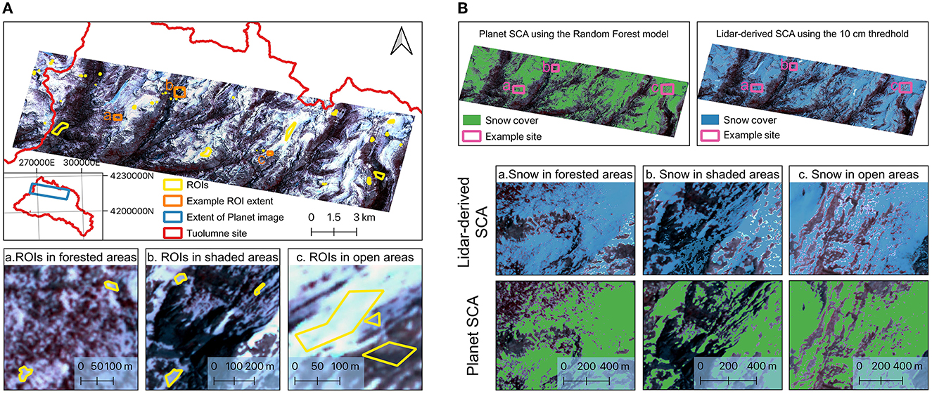
Figure 4. (A) The cloud-free PlanetScope image of the Tuolumne site on 28 May 2018, which was used for generating training samples. The polygons (yellow) represent sample ROI polygons with three typical land types shown in zoomed views for corresponding locations in (a–c). (B) Spatial distribution of modeled SCA and SCA extent derived from contemporaneous ASO snow depth data (ASO_3M_SD_USCATE_20180528), which were used as “ground truth” for model validation. The zoomed views in (a–c) provide details for the corresponding locations in the Planet image in (B).

To get an optimal set of model parameters, we conducted a series of sensitivity tests on the four main parameters to determine their effect on overall model accuracy. Ultimately, we finalized the model with all samples, four features, 10 trees, and a maximum depth of ten. Readers can refer to the Code and Data Section for more detailed information about model parameter tuning. After 1,000 repeated K-fold cross-validation, the fine-tuned model achieved reliable performance with overall precision, recall, and F1 score higher than 0.99. Details of the three evaluation metrics and their equations are introduced in Section 3.3.

3.3. Evaluate model accuracy using ASO snow depth data

3.3.1. Overall model performance

To generate reference SCA maps across the four study sites, we used the 10 cm snow depth threshold to classify snow vs. snow-free extent from the 3-m snow depth data provided by the ASO. Inc (Painter et al., 2016), in which the snow depth threshold was determined following earlier studies (Cannistra et al., 2021; John et al., 2022).

The following three statistical metrics (Equations 1–3) were used to represent model performance.

\begin{array}{l} P r e c i s i o n = \frac{T P}{T P + F P} & (1) \end{array}

where TP represents true positives, and FP represents false positives. Precision (Equation 1) is the proportion of predicted snow pixels that are correctly classified and is used to measure commission-error, which refers to the pixels observed as snow-free but predicted as snow. Lower precision values usually correspond to higher commission-error.

\begin{array}{l} R e c a l l = \frac{T P}{T P + F N} & (2) \end{array}

where FN represents false negatives. Recall (Equation 2) is the proportion of actual snow pixels that are predicted as snow correctly and is also known as the true positive rate. Recall is used to measure omission-error, which refers to the pixels observed as snow but predicted as snow-free. Lower recall values usually correspond to higher omission-error.

\begin{array}{l} F 1 s c o r e = \frac{2 \times P r e c i s i o n \times R e c a l l}{P r e c i s i o n + R e c a l l} & (3) \end{array}

where F1 score (Equation 3) combines both precision and recall metrics into one single score, providing a more balanced measurement of model performance. The harmonic mean is used to calculate the F1 score, which gives more weight to lower values, making it a more suitable metric for imbalanced datasets where the number of samples in one class is significantly higher than the other. In our case, when the snow and snow-free classes are heavily imbalanced and detecting true snow pixels is more critical than detecting snow-free pixels (such as during the late snow season), F1 score remains a powerful evaluation metric for model evaluation. However, when TP equals 0, which indicates no snow on the ground, the F1 score becomes an inappropriate metric for evaluating model performance.

To evaluate the accuracy of the mapped SCA, we calculated all three metrics for all 103 PlanetScope images from the four study sites. The three metrics range from 0 to 1, with higher values indicating better model performance.

3.3.2. Model performance in meadow areas

We hypothesized that the accuracy of snow cover mapping in meadows may be affected by their size and shape complexity, considering the impact of the mixed pixel effect and tree shadows at the meadow edge. To verify this hypothesis, we assessed model accuracy across different meadow sizes and shape complexities. To represent meadow shape complexity, we introduced a parameter known as the perimeter–area ratio (PAR), which considers the proportion of meadow area exposed to edges, where we anticipate larger snow mapping errors due to the tree shadows and mixed pixels. If two meadows are of the same size, a larger perimeter, indicating more pixels located at meadow edges, would increase the PAR, potentially decreasing model accuracy.

There were 2018 meadows larger than 4 × 10⁴ m² (i.e., one acre) located across the Tuolumne area, and 1,805 meadows across the San Joaquin site, in the SNMMPC dataset (details provided in Section 2.2.3). Since the coverage of PlanetScope images on each ASO date was different, and some meadows might have been accounted for multiple times on different dates, we treated each meadow on a specific PlanetScope image as an independent object. A total of 18,512 meadow objects were analyzed for the two study sites. To reduce the influence of outliers, we removed the meadows that exceeded the 90th percentile of meadow size (14.3 acres) and complexity (PAR = 0.1 m⁻¹), based on meadows within the two study sites. We also removed 96 meadows without snow cover because when there is no true positive (lidar-derived snow pixel), all statistical metrics would be 0, resulting in an inappropriate evaluation. We classified the remaining 7,741 meadows into 10 groups based on their size and shape complexity, respectively. We then fitted linear regression models between the median F1 score of each group and the mean value of each group's meadow size and shape complexity. We selected 10 as the group size to ensure that each group had sufficient meadows to accurately represent the characteristics of the group.

3.3.3. Model performance in forests

To assess the model performance in forest edges and gaps, we classified the study sites into six categories (Table 2) based on the distance to the canopy edge, DCE (Mazzotti et al., 2019). We calculate DCE using the ASO CHM dataset, following the method developed by Mazzotti et al. (2019; see Section 2.2.2 for details]. DCE represents the distance of a pixel from the edge of a forest to the target pixel. We defined “forest” as pixels with a canopy height higher than 2 m, and “open” as pixels with a canopy height lower than 2 m, which includes bare ground, grassland, shrubland, and small trees (Broxton et al., 2015; Currier and Lundquist, 2018; Mazzotti et al., 2019). We assumed that PlanetScope images have the potential to observe snow in regions with a canopy height lower than 2 m, even when those regions may be partially covered by vegetation. Pixels classified as “forest” would mostly be covered by tree canopy in a 3 by 3 m pixel, based on a scaling exponent between tree height and diameter (Hulshof et al., 2015; Chen and Brockway, 2017). Therefore, 2 m is a reasonable forest height threshold to distinguish “forest” from “open” (Broxton et al., 2015; Currier and Lundquist, 2018; Mazzotti et al., 2019). We excluded areas with a DCE higher than 100 m, as they were far enough away from the forest to be considered wide-open areas where the model accuracy would not be influenced by DCE. Additionally, we excluded areas with a DCE < −9 m, given that optical sensors are not suitable for mapping ground surface features obscured by dense forest canopies.

TABLE 2

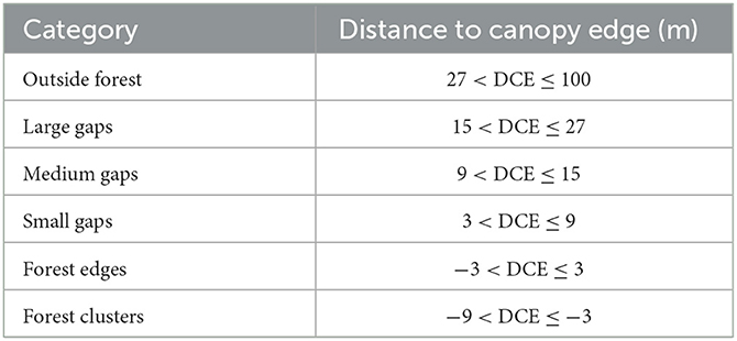
Table 2. Land types in forested areas are based on the distance to canopy edge.

To keep SCA evaluation concise, we only presented F1 scores for the meadow and forest areas because F1 scores provide a comprehensive assessment of overall SCA accuracy, considering both commission-errors (i.e., precision) and omission-errors (i.e., recall). We also calculated percentage bias (PBIAS, Equation 4) in the forested areas to provide an overall estimate of SCA bias.

\begin{array}{l} P B I A S = \frac{S C A_{p l a n e t} - S C A_{l i d a r}}{S C A_{l i d a r}} \times 100 & (4) \end{array}

where SCA_planet is the mean SCA for a specific region mapped from PlanetScope images, while SCA_lidar is the mean SCA derived from ASO lidar data.

4. Results

4.1. Overall SCA accuracy at the four study sites

Our model achieved a median F1 score, precision, and recall of 0.75, 0.91, and 0.70, respectively (Figures 5A–C), demonstrating good performance in mapping snow cover across mountainous terrain at a 3-m spatial resolution. The uncertainty of mapped SCA was dominated by omission-errors, as revealed by the much lower recall values than the precision values (Figures 5B, C). Notably, more than 90% of the images exhibited precision values higher than 0.75, indicating that the model produced consistently small commission-errors. Moreover, while the distribution of recall across images peaked at a high value of 0.81 (Figure 5C), its distribution was widely spread, primarily due to the high omission-errors in under-canopy areas (Figures 5F, I). When the under-canopy areas were excluded from the analysis, the model showed much better and more robust performance, with a median F1 score of 0.82 (Figure 5D). Compared to the overall model performance across all areas, omission-errors in open areas were reduced (Figure 5F), while commission-errors showed little difference (Figure 5E).

FIGURE 5

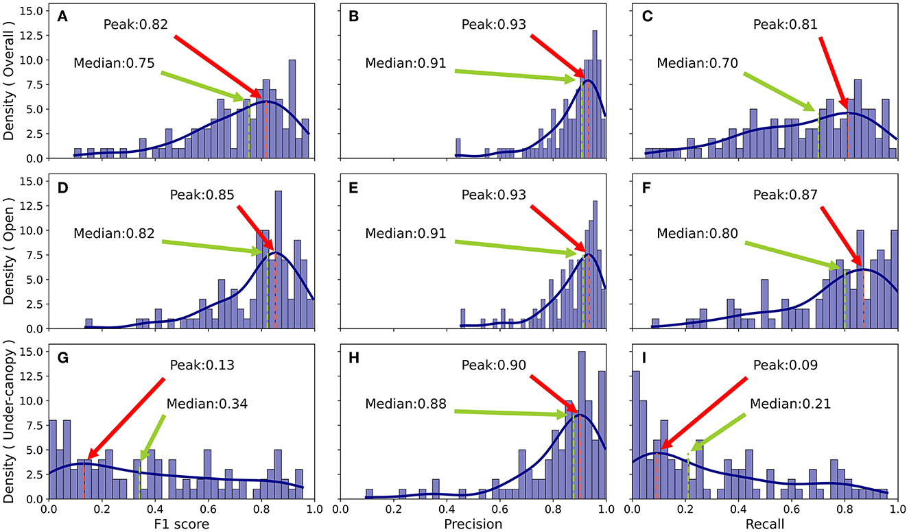
Figure 5. Distribution of model evaluation metrics F1 score, Precision, and Recall for all 103 PlanetScope images across four study sites, with the rows corresponding to statistics for overall (A–C), open (canopy height ≤ 2m) (D–F), and under-canopy regions (canopy height > 2m) (G–I), while the columns represent each performance metric. The median value for each metric is indicated by a green arrow and a dashed line, while the highest concentration of data (based on kernel density estimation) is denoted by a red arrow and a dashed line. The density plots provide a visual representation of the probability distribution of the metrics across the images.

Across the four study sites, the model exhibited the best overall performance at the Engadin site, which had the lowest forest coverage and smallest size (Table 1), with the highest F1 score of 0.90 ± 0.06. While the precision value at the Engadin site was relatively lower than that of the Tuolumne and Gunnison sites, its recall value (0.92 ± 0.04) was notably higher than the other three sites, indicating minimal omission errors in mapping SCA. This can be partially explained by snow-free ground under canopy indicated by lidar-SCA, as the satellite images were collected on March 17, after most snow in low-elevation forested areas had melted.

While the Tuolumne site had the worst overall accuracy among the four studied sites, with an overall F1 score of 0.68 ± 0.20 (Table 3), it had a relatively accurate SCA for open areas, with an F1 score of 0.75 ± 0.18 (Table 3). The low overall SCA accuracy across Tuolumne could be partially explained by the inclusion of a larger number of images in the evaluation, some of which had high forest coverage, a high percentage of terrain shadows, or low solar illumination conditions, all of which could increase omission errors.

TABLE 3

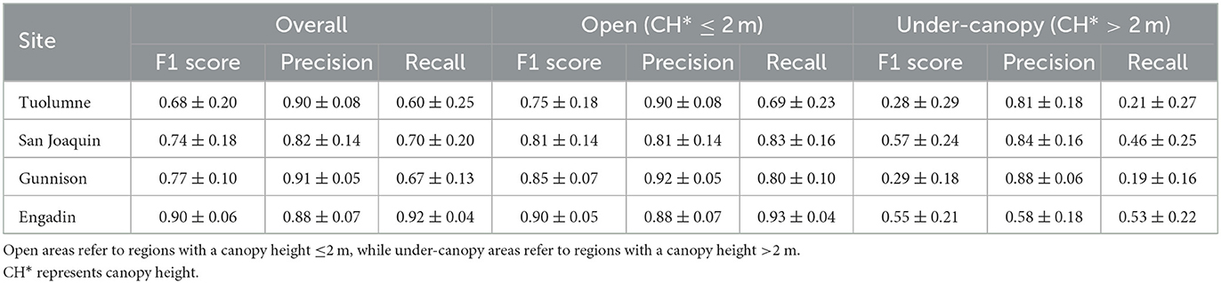
Table 3. Model performance at the four study sites is represented by the mean and standard deviation of each statistical metric.

The F1 score, precision, and recall value for the image that we used to train the model at the Tuolumne site were 0.81, 0.93, and 0.72, respectively, all of which were only slightly higher than the median values of all 103 images tested. This suggests that the model had a very good transferability across geographic locations (Figures 5A–C). Among all four sites, the difference in model performance was less noticeable in open areas (6% in F1 score) compared to under-canopy areas (33% in F1 score).

To better understand the model's performance across space, we selected three example sites in Tuolumne on July 5, 2019, when the watershed was partially covered by snow (Figure 6). Mapping SCA in the late snow season can be challenging due to the reduced snow surface reflectance caused by larger snow grain size or higher accumulation of light-absorbing particles such as black carbon, mineral dust, or coniferous leaf litter. Additionally, since a big portion of the ground is partially covered by snow, the mixed pixels can be notable and further challenge the accuracy of SCA mapping in the late snow season. Despite these challenges, the PlanetScope-derived SCA showed good agreement with the lidar-derived SCA for all three example locations, even in small forest gaps (Figure 6A) and small snow patches (Figure 6C). Only a small portion of pixels showed disagreement between lidar-derived SCA and Planet-derived SCA and were mostly located at the edges of snowpack and under-canopy areas. Commission-errors were mainly found at the edges of forests (Figure 6A) and snow patches (Figure 6B), while omission-errors were mainly found in the forested areas (Figure 6C).

FIGURE 6

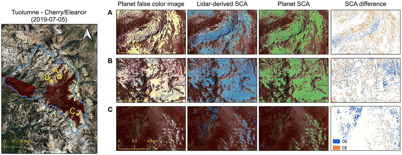
Figure 6. Examples of the spatial distribution of snow in PlanetScope images. The left panel presents cloud-free PlanetScope images from July 5th, 2019, overlaid on a Google Satellite base map. A False color scheme using the NIR, red, and green bands highlights vegetation in red and makes it easier to distinguish it from snow. Rows (A–C) demonstrate the performance of the RF in mapping SCA at three example sites, with a specific focus on open, shaded, and forested areas, respectively. The right panel has four columns: Planet false color images, binary SCA derived from ASO snow depth using a 10 cm threshold, binary SCA derived using our RF model for the PlanetScope image, and the difference between lidar-derived SCA and Planet SCA. The legend OE and CE refer to omission errors and commission errors, respectively.

4.2. SCA accuracy in meadow areas

Within the 7,741 studied meadows in Tuolumne and San Joaquin, the median F1 score, precision, and recall were 0.85, 0.97, and 0.82, respectively, which are comparable to the model performance in open areas (CHM < 2 m) across the four sites (Figure 5). While the model's performance varied notably within each group, the overall accuracy of SCA mapping in meadows showed a significant increasing trend as meadow size increased or meadow shape complexity decreased, as revealed by the best-fit lines between the median F1 score and the mean value of the grouped meadow size (Figure 7A) and shape complexity (Figure 7B).

FIGURE 7

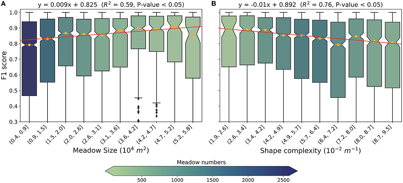
Figure 7. Relationships between mapped SCA accuracy with the meadow size (A) and meadow shape complexity (B). SCA model accuracy is represented by the F1 score, and the shape complexity is represented by the perimeter-area ratio (PAR). Each boxplot represents a group of meadows falling within the range of meadow size or shape complexity labeled on the x-axis. The boxes are colored based on meadow numbers according to the color scheme shown in the legend. The red lines represent the best-fit line between the median F1 score and the mean values of the grouped meadow size (A) and shape complexity (B).

The F1 score for meadows in the size range of 5.2 – 5.8 × 10⁴ m² (13.0 – 14.0 acre), the largest meadow group, was found to be 9% more accurate than the smallest meadow group, which includes meadows in the size range of 4 – 9 × 10³ m² (1.0 – 2.0 acre; Figure 7A). The median F1 score for meadows larger than 1.5 × 10⁴ m² (3.8 acres), the median size of meadows studied, was 0.90, representing an 11% increase compared to smaller meadows. However, it is noticeable that the SCA accuracy in the largest meadow group was lower than that in a few other groups with smaller meadow sizes. This can be partially explained by the fact that meadow size is not the only factor that impacts SCA mapping accuracy. Moreover, the model performance in the largest meadow group was evaluated based on a relatively small number of meadows (i.e., 121, or 1.6% of the total meadows), which may not be representative due to the small sample size. Furthermore, the shape complexity of meadows also impacted SCA accuracy, with meadows with the simplest geometry (1.9 – 2.7 × 10⁻² m⁻¹) showing 10% more accuracy compared to those meadows with the most complex geometry (8.7 – 9.5 × 10⁻³ m⁻¹) (Figure 7B).

4.3. SCA accuracy in forest edges and forest gaps

The model showed a robust performance in mapping SCA for areas located at a distance of at least 3–4 pixels (~10 m) away from forest edges (Figure 8). In the under-canopy portion, where the PlanetScope images were not expected to detect snow, the F1 score was low, and the overall PBIAS was negative. Notably, the F1 score showed a dramatic increase in the transition zone, which spanned ~3–4 pixels on PlanetScope imagery (equivalent to about 10 meters; Figure 8A). When the DCE exceeded 10 meters, the F1 score remained stable across all four sites. Moreover, the overall PBIAS for the Gunnison and Engadin sites was close to 0%, whereas Tuolumne showed a small negative PBIAS, and San Joaquin had a small positive PBIAS (Figure 8B). Although many other factors may influence mapped SCA accuracy, for satellites like the PlanetScope constellation at the about 3-m spatial resolution, the model can provide more robust SCA information for areas located more than 10 m away from forest edges.

FIGURE 8

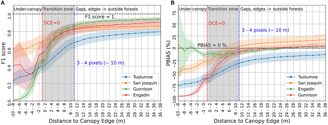
Figure 8. Relationships between model performance and the distance to canopy edge (DCE) for all pixels at the four study sites. The model performance is measured using the F1 score (A) and the percentage bias (PBIAS) (B) of each DCE group. The shaded areas on each curve represent the range of values within one standard deviation of the F1 score (left) and PBIAS (right) of the images tested at each site. The under-canopy region refers to DCE values below 0 m; the transition zone, shaded in gray, encompasses DCE values from 0m to 10m; and the forest gaps and edges to outside forests refer to DCE values higher than 10m.

The model showed a promising capacity for mapping snow cover in forest gaps, which refer to areas with 3 m < DCE < 27 m or 1–9 pixels away from forest pixels, as shown in Figure 9. The median F1 scores for large forest gaps (15 m < DCE < 27 m) were 0.82, 0.86, 0.87, and 0.93 for the Tuolumne, San Joaquin, Gunnison, and Engadin sites, respectively. Despite higher SCA uncertainties in medium and small forest gaps compared to large gaps, the model still demonstrated a reliable ability to map SCA in those regions, with median F1 scores of 0.72 and 0.82 across the four sites, respectively. For small forest gaps (3 m < DCE < 9 m), where the model performance was relatively poor, the median F1 score was 0.62, 0.79, 0.80, and 0.77 for the Tuolumne, San Joaquin, Gunnison, and Engadin sites, respectively.

FIGURE 9

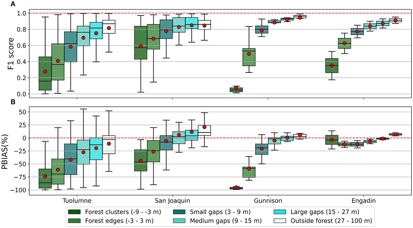
Figure 9. Model performance within defined land type in forested areas for the four study sites. The red dots represent the mean F1 score (A) and percentage bias (PBIAS) (B) of each land type on one PlanetScope image. The boxplot represents the range of F1 score and PBIAS of each land type across all the PlanetScope images used for each study site.

The overall PBIAS for small, medium, and large forest gaps and areas outside forests was relatively low for all sites, particularly for Gunnison and Engadin, while forest clusters and forest edges showed large negative PBIAS (Figure 9B). Overall, the SCA accuracy increased with distance from the forest edge and toward open areas, and the model performed worst in deep forest clusters (−9 m < DCE < −3 m) and forest edges (−3 m < DCE < 3 m), where the ground surface is obstructed by tree branches.

5. Discussion

5.1. Overall model performance

High spatiotemporal resolution snow cover data is critical for studying water availability and changes in plant phenology in seasonal snow-covered ecosystems, such as montane forests and meadows. In this study, we investigated the performance of a Random Forest (RF) model in mapping SCA over meadows and forests using PlanetScope imagery. The RF model achieved comparable performance with prior studies that applied more sophisticated and computationally expensive methods (Cannistra et al., 2021; John et al., 2022). For the open areas in the Gunnison site where we used almost the same Planet images as that of Cannistra et al. (2021), RF achieved an F1 score of 0.85, precision of 0.92, and recall of 0.80, while the CNN-based method reported slightly lower performance with an F1 score of 0.82, precision of 0.88, and recall of 0.77 recall. However, the performance of the CNN-based method could be improved by including additional information, such as the Normalized Difference Vegetation Index (John et al., 2022).

Including samples from different dates and locations in the training of the RF model may have the potential to improve SCA accuracy in more diverse conditions. However, new features like dates or locations may be necessary to account for the differences in environmental conditions. For simplicity and proof of concept, in this work, we only used one image to train the model and explored the Random Forest algorithm's capability in snow mapping with the assumption that it could be extended to a bigger training dataset. The RF model showed good transferability across four study sites, as demonstrated by the validation results in Table 3, and proved efficient for identifying snow in meadows and forest gaps. The model was trained on one PlanetScope image and applied to 103 images, of which 61% had an F1 score higher than 0.80 in open areas (canopy height < 2 m). The model's inability to accurately predict snow cover in under-canopy areas is expected since passive optical sensors, like those used in the PlanetScope Constellations, cannot penetrate forest canopy (Figure 5G).

Our model showed much higher omission-errors than commission-errors. The primary reasons for the omission errors in SCA mapping from Planet imagery are the canopy obstruction and the presence of mixed pixels of snow and trees at forest edges. Other factors such as illumination conditions and landscape shadows caused by mountain terrain, tall trees, and cloud cover can further exacerbate the problem and lead to omission-errors (Raleigh et al., 2013; Hall et al., 2019; Zhang et al., 2021; Luo et al., 2022). Mapping SCA can be challenging under low illumination and landcover shadows, as snow pixels and snow-free pixels have different reflectance characteristics compared with those in open spaces with good illumination conditions (Raleigh et al., 2013; Hall et al., 2019; Zhang et al., 2021; Luo et al., 2022). Additionally, our model is limited to cloud-free images because the PlanetScope images do not have a shortwave infrared band, which is necessary to distinguish snow from clouds. Planet provides a cloud mask for each image, which could be helpful in SCA mapping. However, future studies are needed to assess the accuracy of the cloud masks.

5.2. Model validation sensitivity

To understand the impact of the snow depth threshold on the model validation results, we performed a sensitivity analysis on a randomly selected PlanetScope image (20180528_181110_1025_3B). In this analysis, we evaluated Planet-derived SCA using lidar-derived SCA with threshold ranges from 1 to 15 cm (Supplementary Figure 1). This range covers the thresholds used in previous studies to generate snow extent from ASO lidar snow depth data (Cristea et al., 2017; Kostadinov et al., 2019; Cannistra et al., 2021; John et al., 2022). Because the optical sensors, like those used by PlanetScope, cannot see the under-canopy ground, we excluded forested areas for the sensitivity analysis.

The sensitivity analysis showed that precision decreased while recall increased as the threshold increased (Supplementary Figure 1). The overall F1 score showed an increasing trend with the increase of threshold. However, only a small difference (1.2 km² or 0.8%) in lidar-derived SCA was observed between using a 1 and 15 cm threshold. The difference in F1 score was also negligible at 0.01 or 0.29%, indicating that using a 10 cm threshold to derive snow cover from the lidar-derived snow depth data was a reliable and reasonable selection for model validation (Cannistra et al., 2021; John et al., 2022).

The 103 validation images were acquired by three different generations of PlanetScope instruments (Figure 2). While the band configurations varied slightly among the three PlanetScope satellite instruments (Figure 2), our model proved suitable for mapping SCA for all three generations with high accuracy (Supplementary Figure 2). For example, the median F1 scores for PS2, PS2.SD, and PSB.SD were 0.77, 0.67, and 0.76, respectively. While training separate models for different PlanetScope instruments could further improve SCA mapping accuracy, we chose not to do so, as we aimed to examine the universality of the model and ensure its high applicability and simplicity. The impact of sensor discrepancy will become even more negligible in newer products, such as the harmonized PlanetScope product that matches the spectral responses of Copernicus Sentinel-2 (Moon et al., 2021).

We performed a basic image screening to remove images that were significantly contaminated by cloud cover or showed low spectral quality (11% of the total image collection). The overall model accuracy could be further improved by implementing a more stringent screening process, given the reported data quality issues such as image saturation artifacts and scene-to-scene misregistration, as well as inconsistency in geolocation accuracy and parallax-induced offsets between spectral bands (Frazier and Hemingway, 2021; Aati et al., 2022). For example, the misaligned geolocation of different spectral bands, which is particularly noticeable for the pixels located at the ridge of the mountains and at the edge of snowpacks in Dove-R and SuperDove images, is likely to cause commission errors if the “real” ground is not covered by snow (snow-free; Figure 6).

5.3. SCA in meadows and forest gaps

Our study is motivated by the growing volume of high-resolution satellites data at the sub-meter to meter scale (Baba et al., 2020; Cannistra et al., 2021; Li et al., 2021; Hu and Shean, 2022; John et al., 2022), which shows a high potential for mapping snow cover in mountain ecosystems like meadows and forests. Changes in snow cover distribution over time and space can result in significant differences in the spatial variability of soil moisture and soil temperature, thereby affecting the timing and location of plant emergence in these ecosystems. Driven by the interaction of snowfall, wind, vegetation, and terrain, mountain snow cover and snowmelt time often show high spatial heterogeneity even at fine scales (< 10 m). By analyzing high-resolution PlanetScope images, we can observe spatial and temporal changes in snow cover, which can inform plant phenology monitoring in mountainous meadows and forest gaps.

Our study only considers the impact of meadow size and geometry on SCA mapping accuracy. It is worth mentioning that other factors may also influence SCA accuracy in meadow areas. For example, the decrease in SCA accuracy for the largest meadows (Figure 7) could be due to the increase of mixed pixels. The meadow areas in Figure 7 are large enough that wind redistribution of snow cover creates a patchier snow cover, resulting in more mixed pixels, which are always more challenging to classify than pure snow or snow-free pixels. The height and types of trees surrounding the meadows can cause different shadow and mixed pixel conditions, potentially affecting SCA accuracy. Additionally, the presence of different land cover types within meadows, such as streams, as well as differences in snowmelt timing, may also lead to the occurrence of more mixed pixels, which can further affect the accuracy of SCA mapping.

While mapping snow using optical satellite images in forested areas remains challenging due to the obstruction caused by tree canopies, we were able to derive snow cover in areas as close as 10 m from trees, as well as in relatively large forest gaps (i.e., 15 m < DCE < 27 m) using PlanetScope imagery. Airborne or UAV lidar-derived snow depth data may provide better estimates of SCA under-canopy (Cristea et al., 2017; Kostadinov et al., 2019; Cannistra et al., 2021; Koutantou et al., 2021; John et al., 2022), but the spatial coverage of the flights was limited to the available budget. Canopy adjustment approaches are also commonly used to estimate under-canopy snow cover based on viewable SCA or viewable snow fraction, which assumes that the snow cover in open areas is the same as under-canopy snow cover within one pixel (Painter et al., 2009; Nolin, 2010; Raleigh et al., 2013; Rittger et al., 2020). With high-resolution PlanetScope SCA maps in forest gaps, we will better understand snow cover distributions in forested areas, which could inform future canopy adjustments to get a better estimate of under-canopy snow cover. Additionally, high spatial and temporal fusion datasets, such as the Harmonized Landsat and Sentinel-2 product, offer new opportunities for mapping SCA in the meadow and forested areas.

The overlap of meadows and forests with seasonal snow makes snow cover a critical factor in controlling the eco-hydrological process at high latitudes and in alpine regions. Recent studies have documented significant changes in the compositions and structures of vegetation species due to reduced snow cover, earlier snow disappearance, and drier soil moisture (Chen et al., 2008; Myers-Smith et al., 2011; Sherwood et al., 2017; Amagai et al., 2018). Earlier snowmelt could lead to earlier plant emergence and development, which increases the risk of plants' exposure to lower air temperatures in winter and early spring, resulting in more frequent and serious frost damage and reducing plant reproduction rate. Therefore, a series of high spatiotemporal resolution maps of mountain snow cover can support future analysis of the spatial diversity of plant communities and studies on meadow or forest ecosystem functions (Loheide and Gorelick, 2007; Loheide and Lundquist, 2009; Lowry et al., 2011; Blackburn et al., 2021).

6. Summary and conclusion

To advance snow cover mapping in mountainous areas, we developed a machine learning model to map SCA using PlanetScope imagery at a 3-m spatial resolution and explicitly evaluated the mapped SCA accuracy in montane meadows and forest gaps. The PlanetScope-derived SCA showed good agreement with SCA derived from a lidar snow depth dataset over four study sites in the Western United States and Switzerland, with a median F1 score of 0.75 for all 103 PlanetScope images. Tree canopy obstruction caused the main omission-errors for SCA mapping, as indicated by the median recall values of 0.21 and 0.80 for under-canopy and open areas, respectively. The model performed much better in open areas with a relatively high median F1 score of 0.82.

The use of high-resolution PlanetScope imagery showed promising capability for mapping SCA in montane meadows and forest gaps. The model had an overall median F1 score of 0.83 for 7,741 studied meadows at the Tuolumne and San Joaquin sites. SCA accuracy in meadow areas was influenced by the meadow size and meadow shape complexity. Mapped SCA for larger and more simply shaped meadows was generally more accurate than that for smaller and more complexly shaped meadows. The median F1 scores in forested areas were higher for large gaps (i.e., 15 m < DCE < 27 m) than for small gaps (i.e., 3 m < DCE < 9 m). Specifically, the median F1 score for large forest gaps at the Tuolumne, San Joaquin, Gunnison, and Engadin sites were 0.82, 0.86, 0.87, and 0.93, respectively, which were at least 8% higher than those for small forest gaps. While mapping SCA accurately over regions close to or under forest canopy remains challenging, the proposed RF model could provide robust SCA information for the very close regions (>10 m) to the forest edges and relatively large forest gaps (i.e., 15 m < DCE < 27 m). This advance in our snow mapping capabilities in montane forests will have profound implications for future ecohydrological studies.

7. Code and data

The reproducible SCA mapping model and code are available on GitHub (https://github.com/KehanGit/High_resolution_snow_cover_mapping.git). The tutorial Jupyter Notebook is published as a GeoScience Machine Learning Resources and Training “use case book” in the GeoSMART GitHub repository and hosted on GitHub pages (GeoSMART, https://geo-smart.github.io/scm_geosmart_use_case/). More information about the GeoSMART organization, methods to get in contact, and resources for advancing machine learning use in the geosciences can be found on the website at geo-smart.github.io.

To improve the reproducibility and reusability of the SCA mapping application, we adopted a workflow management tool—Geoweaver (Sun et al., 2020, 2022), to rebuild the SCA mapping workflow. The SCA mapping workflow is available on GitHub (https://github.com/geo-smart/sca_mapping_geoweaver) and users can download the latest released zip file and import it into Geoweaver to browse and run. Geoweaver allows convenient sharing of everyone's progress among team members without losing details and model run history, as source code, model history, and output logs are all saved to a local database that is easily portable. We hope the adoption of Geoweaver can greatly improve the FAIRness of the SCA workflow for the scientific community and help serve as a valuable community asset fostering collaborative, reproducible future research.

The PlanetScope images used in this study are accessible through the NASA Commercial Smallsat Data Acquisition (CSDA) program or the Planet Education and Research program, and the SCA maps will be made available in a Zenodo repository.

Data availability statement

The original contributions presented in the study are included in the article/Supplementary material, further inquiries can be directed to the corresponding author.

Author contributions

KY and NC contributed to the conception and design of the study. KY organized the database, performed the statistical analysis, and wrote the first draft of the manuscript. All authors contributed to manuscript revision, read, and approved the submitted version.

Funding

This work was supported by the NSF grants NSF EAR−1947875 and NSF OAC−2117834, the NASA grant #80NSSC21K1151, and the eScience Institute Data Science Fellowship at the University of Washington.

Acknowledgments

We gratefully acknowledge Clare Webster and Giulia Mazzotti for providing the canopy height model and snow depth data for the Engadin site in Switzerland. We gratefully acknowledge Tanya Harrison with Planet Labs and Kat Bormann with ASO Inc for their help and support in providing access to the Planet satellite imagery and snow depth data, respectively.

Conflict of interest

The authors declare that the research was conducted in the absence of any commercial or financial relationships that could be construed as a potential conflict of interest.

Publisher's note

All claims expressed in this article are solely those of the authors and do not necessarily represent those of their affiliated organizations, or those of the publisher, the editors and the reviewers. Any product that may be evaluated in this article, or claim that may be made by its manufacturer, is not guaranteed or endorsed by the publisher.

Supplementary material

The Supplementary Material for this article can be found online at: https://www.frontiersin.org/articles/10.3389/frwa.2023.1128758/full#supplementary-material

References

Aalstad, K., Westermann, S., and Bertino, L. (2020). Evaluating satellite retrieved fractional snow-covered area at a high-Arctic site using terrestrial photography. Remot. Sens. Environ. 239, 111618. doi: 10.1016/j.rse.2019.111618