Hydraulic head change predictions in groundwater models using a probabilistic neural network

Groundwater resource management is an increasingly complicated task that is expected to only get harder and more important with future climate change and increasing water demands resulting in an increasing need for fast and accurate decision support systems. Numerical flow simulations are accurate but slow, while response matrix methods are fast but only accurate in near-linear problems. This paper presents a method based on a probabilistic neural network that predicts hydraulic head changes from groundwater abstraction with uncertainty estimates, that is both fast and useful for non-linear problems. A generalized method of constructing and training such a network is demonstrated and applied to a groundwater model case of the San Pedro River Basin. The accuracy and speed of the neural network are compared to results using MODFLOW and a constructed response matrix of the model. The network has fast predictions with results similar to the full numerical solution. The network can adapt to non-linearities in the numerical model that the response matrix method fails at resolving. We discuss the application of the neural network in a decision support framework and describe how the uncertainty estimate accurately describes the uncertainty related to the construction of the training data set.

1. Introduction

Resolving the complexity of flow in a groundwater reservoir is a challenging but important task for securing water supply around the world. Societies utilize groundwater for drinking water supply, agriculture, and environmental control on a large scale. Proper groundwater management prevents depletion or pollution of the resource and saves societies millions of dollars in the remediation of contaminated areas (Sun and Zheng, 1999). Therefore, practitioners often use numerical models as decision support tools for planning and managing groundwater (Hadded et al., 2013). Numerical models can simulate flow dynamics and forecast the effects of management strategies. They can act as decision support tools for tasks such as finding the optimal location for a new well or estimating the effects on wetland and stream depletion. Setting up accurate numerical models requires high numerical grid resolution which comes at the price of long computation times for flow calculations and high memory demand (Cheng et al., 2014). As an example, Bakker et al. (2016) perform a capture fraction analysis of a groundwater model using the flow simulation code MODFLOW (Harbaugh, 2005). Here, 1,530 model runs took approximately 10 h, which is impractical for rapid decision support.

Because of the long computation time, management models can be approximated using the response matrix (RM) approach (Gorelick, 1983). The approach is based on the assumption of space superposition and uses single simulations of wells to calculate coefficient values that linearly relate a pumping rate at one point to drawdown at different locations in the model (Psilovikos, 2006). Once the RM is constructed, it can replace the simulation code and perform fast forward calculations. The implicit assumption of linearity between pumping rate and drawdown in the RM approach is valid in simpler cases, but as model non-linearities increase the assumption of this linear relation diminishes (Niswonger et al., 2011) and the linear assumption becomes less accurate. In practice, this limits the practical use of the RM system and calls for different approaches that run fast and can resolve non-linear problems.

Neural networks started gaining traction in water resources in the 1990s as described in the review by Maier and Dandy (2000). Within water resources management, Rogers and Dowla (1994) applied a neural network as a tool to search for optimal pumping strategies for aquifer remediation. The study used model-simulated data to train the network and found results consistent with conventional methods. They point out the lower computational burden of the Artificial Neural Network (ANN) approach as an advantage to the conventional technique. A different approach is to use historical data as training inputs (Yoon et al., 2011; Chen et al., 2020). Research has shown, that these networks, in some cases, outperform numerical flow models in predictive accuracy and are easier to develop (Coppola et al., 2003; Mohanty et al., 2013). Recently, applications of deep neural networks are advancing in hydrology. A study by Dagasan et al. (2020) makes use of a newer and advanced type of network called Generative Adversarial Networks (GANs) as a replacement for a forward operator in a hydrogeological inverse problem. The trained network shows capabilities of mapping hydraulic conductivity fields to corresponding flow simulations with significant time savings as opposed to MODFLOW. Lykkegaard et al. (2021) show that the combination of Markov chain Monte Carlo (MCMC) and deep neural networks can reduce the cost of uncertainty quantification for groundwater flow models by up to 50% compared to using a regular Metropolis algorithm. Reductions in computational costs are also mentioned as a great advantage of deep networks (Marais and de Dreuzy, 2017). However, deep networks require large amounts of training data to obtain high accuracy, and networks such as GANs can require significant training times.

Other options within supervised learning for water resources include e.g., support vector machines, random forest methods, and regression trees. These methods also prove capable of understanding non-linear relationships between water quality parameters and complicated measurements such as nitrate distribution in groundwater or oxygen demands for a healthy biological system (Knoll et al., 2019; Najafzadeh and Niazmardi, 2021). With all these possibilities, it can be difficult to select the optimal method for a given problem without performing a comparison analysis. However, if the goal is to simply investigate whether the problem is solvable or not using supervised learning, a Multilayer Perceptron Neural Network (MLP-NN) can approximate any function to an arbitrary accuracy (Hornik et al., 1990). This makes the MLP-NN ideal as the first choice for new investigations, where success is not guaranteed.

Previous studies have already implemented model-simulation trained neural networks to handle groundwater management tasks in non-linear problems that can replace the RM approach (Chu and Chang, 2009; Chen et al., 2013). They focus on predicting the non-linear temporal change caused by well-systems in an aquifer and apply the trained neural network in optimization policy algorithms. The results are very promising in accuracy and speed, but are case specific to one well-system from where time-series data are simulated for training. These networks can to some extent replicate numerical computations, but lack the flexibility to e.g., simulate different well-systems in new locations. Furthermore, it can be difficult to verify the network predictions without comparing these to numerical simulations or real world observations. We see a need for more spatially flexible neural networks that can understand the impact from groundwater abstraction in user specified well locations and presents a way of validating the trustworthiness of the results.

This study aims to provide fast and highly accurate predictions of hydraulic head changes using a neural network that has applications in a decision support system. Initially, we explain the method behind acquiring data, training, and predicting using the network. We propose to use a few selected attributes in the groundwater model as input features and construct an MLP-NN (Gardner and Dorling, 1998) as a mapper between these features and changes in hydraulic head in a groundwater model. The MLP-NN is trained with model-simulated results of head changes obtained using MODFLOW for a specific test case. As the use of a low-dimensional feature space, leads to a non-unique relation between features and hydraulic head, the network output is a probability distribution (a mean and variance of a normal distribution) describing the head change, as opposed to a single best estimate. The focus of this study is not to design and train a neural network that can be applied in any groundwater model, but instead to document a methodology, where an MLP-NN can replace the heavy groundwater flow calculations or the linear RM, for in principle any groundwater model. The speed and accuracy of the MLP-NN predictions are compared to results using MODFLOW and the RM approach and the abilities of the MLP-NN in a decision support framework are investigated. We further elaborate on the possibilities when predicting a distribution of outcomes in terms of validation of predictions and the completeness of the training set.

2. Methods

This paper focuses on the problem of estimating the change in hydraulic head from groundwater abstraction in a well. Assuming that the groundwater system is anisotropic and that the Cartesian coordinate system is aligned in the direction of anisotropy, this problem can be solved using the 3-dimensional groundwater flow equation given in equation (1) as implemented in the groundwater flow simulator MODFLOW.

$\begin{array}{ll}\frac{\partial }{\partial x}\left(K_x\frac{\partial h}{\partial x}\right)+\frac{\partial }{\partial y}\left(K_y\frac{\partial h}{\partial y}\right)+\frac{\partial }{\partial z}\left(K_z\frac{\partial h}{\partial z}\right)+Q_s^{\prime }=S\frac{\partial h}{\partial t}.& (1)\end{array}$

Here K_x, K_y, and K_z are the hydraulic conductivity values along the Cartesian x, y, and z-axis, $Q_s^{\prime }$ is volumetric flux per unit volume representing flow in and out of the groundwater system from e.g., wells. Some contributions to $Q_s^{\prime }$ can be non-linear, and thus be dependent on h, where h is the potentiometric head, and S is the storage coefficient (Harbaugh, 2005). Provided that the aquifer system is unconfined, the storage coefficient will be dependent on h and thus introduce non-linearity into the system. This can also be described as the mapping g from the model space M (representing K, Q, and S) to data space D (representing Δh), such that

$\begin{array}{ll}\text{D}=g(\text{M}).& (2)\end{array}$

The mapping operator g is unique and provides precise predictions but is time-consuming to run and often not feasible to apply in a tool for fast decision making. Therefore, decision-makers typically base their analysis on faster, approximative methods, e.g., the RM method, or reduce the complexity in the decision support design, for example by reducing the number of model scenarios included in the analysis.

2.1. The response matrix method

The response matrix approach (Gorelick, 1983) is based on the assumption of space superposition and uses single simulations of wells to calculate coefficient values α that relate a pumping rate Q at one point to drawdown Δh at different locations in the model (Psilovikos, 2006). Δh at some location i affected by j wells with pumping rates Q can be described on matrix form as

$\begin{array}{ll}\left[\begin{array}{c}\Delta h_1\\ \Delta h_2\\ ⋮\\ \Delta h_i\end{array}\right]=\begin{array}{c}\left[\begin{array}{cccc}{\alpha }_{1,1}& {\alpha }_{1,2}& \cdots & {\alpha }_{1,j}\\ {\alpha }_{2,1}& {\alpha }_{2,2}& \cdots & {\alpha }_{2,j}\\ ⋮& ⋮& \cdots & ⋮\\ {\alpha }_{i,1}& {\alpha }_{i,2}& \cdots & {\alpha }_{i,j}\end{array}\right]\end{array}·\begin{array}{c}\left[\begin{array}{c}{Q}_1\\ Q_2\\ ⋮\\ Q_j\end{array}\right]\end{array}.& (3)\end{array}$

The relationship is a linear addition of all affecting pumping rates, also known as superposition. Once the matrix coefficients α are determined, equation (3) can be solved very fast for different values of Q. This makes the RM method ideal in a decision support system, where high speed and flexibility are necessary to evaluate multiple situations within a short timeframe. The speed of the RM method comes at the cost of assuming linearity between pumping rates and drawdown. In the case of non-linearities, the method will prove inaccurate, meaning that the method is often constrained to a fixed range of pumping rates (Psilovikos, 2006). This limits the possibilities of the RM method and it might not make sense to implement the method in highly non-linear groundwater models. The method leaves space for a new type of approach that can work in both the linear and non-linear domains with the forward runtime as the RM method. As an alternative to using numerically expensive but accurate MODFLOW simulations, and the fast but linear RM method, we suggest designing and training an ANN to provide both fast, accurate, and non-linear estimates of changes in hydraulic head as a response to groundwater pumping.

2.2. A probabilistic neural network approach

This study proposes to use a neural network to predict the hydraulic head changes (with uncertainty) from groundwater abstraction, with the goal to provide a significant reduction in run time compared to numerical flow modeling, while at the same time reproducing non-linear effects that cannot be handled by the RM method.

To achieve this, we suggest reducing the problem using a sparse representation of M, in form of a set of local attributes in an attribute space A to approximate the head change in a single cell and not the full model. A is representative of the hydrological model in a single location, i, and the hydraulic properties between location and well (which will be considered in detail later). Let g_A refer to the mapping between the feature space A, and the data space D. In general, g_A will refer to a non-unique operator, as opposed to g in equation (2), as the feature space A will only approximate the full model M. Hence, several different data can be the result of the same set of features. Therefore, one should represent the outcome of using the features space as model parameters as a probability distribution:

$\begin{array}{ll}{f}_D(\text{D})=g_A(\text{A})& (4)\end{array}$

If an infinitely large training data [A, D] existed, then realizations of f_D(D) could be obtained directly from the training data set, simply by finding all the data that corresponds to a specific set of features. This is naturally not feasible in practice. Therefore, we suggest to construct a neural network that learns the g_A(A) and use it to directly estimate f_D(D) that refer to all possible data responses for a specific set of features. We wish to estimate the non-unique operator g_A(A) with a neural network based operator we refer to as g_nn(A). As an example we make the assumption that f_D(D) can be describe by a normal distribution, such that f_D(D) → N(d_mean, d_std).

The task is then to design a neural network that solves equation (4), that by taking as input a set of features A, can estimate d_mean and d_std that describes f_D(D) as a normal distribution.

To replace the operator g_nn, we consider as an example a fully connected feed-forward neural network, as it has been demonstrated that a neural network with as little as a single hidden layer can approximate any continuous function with arbitrary accuracy (Hornik et al., 1990).

In order to apply the method one thus needs to:

• select a set of low-dimensional attributes, A, representing hydrological variability around and in-between two locations

• generate a large training data set, [A, D], of corresponding sets of input features and hydraulic head changes [a, d] obtained using MODFLOW [Equation (1)]

• design a neural network whose input is a single set of attributes, a, and whose output is two parameters, the mean and standard deviation of a 1D normal distribution describing the change in hydraulic head, d

• train the network.

The hope is that the trained neural network model, g_nn, can be used as an efficient substitute for g(M) in equation (2), when run for all cells in a model. The choice of attributes, and construction of the training data set will be considered later as part of the test case.

2.3. Neural network design

A fully connected Artificial Neural Network (ANN) consist of a number of neurons, ordered in layers. Each neuron has two free parameters, a weight and a bias, that transforms an input into an output using an activation function (Gardner and Dorling, 1998). Training of an ANN consists of adjusting the weights and biases of all neurons in order to minimize a chosen loss function that defines what the ANN is trained to predict.

The fully connected neural network can be split into an input layer, some hidden layers, and an output layer. The design of the input layer, the output layer, and the choice of loss function, is largely independent of the particular groundwater model considered. The input layer simply consist of n_A neurons, referring to the number of features A, where A = [a₁, a₂, …, a_nA]. The output layer consists of two neurons, one neuron for the mean and one for the standard deviation of a normal distribution representing the change in hydraulic head (Specht, 1990; Mohebali et al., 2019). The full probability density function of such a 1D normal distribution is given by

$\begin{array}{ll}P\left(y|\mu ,\sigma \right)=\frac{1}{\sigma \sqrt{2\pi }}{e}^{-\frac{1}{2}{\left(\frac{y-\mu }{\sigma }\right)}^2}& (5)\end{array}$

In order to be able to interpret the outcome of the ANN as a mean, μ, and standard deviation, σ, we would like to maximize equation (5), when evaluated on all sets of data, in the training data set, d, compared to the [d_mean, d_std] estimated from the corresponding set of attributes, a, given g_nn(a). This is similar to minimizing the log-likelihood of equation (5), which is used as the loss function to be minimized when training the ANN, as

$\begin{array}{ll}\text{LOSS}=-logP\left(y|\mu ,\sigma \right)=log\left(\sigma \sqrt{2\pi }\right)+\frac{1}{2{\sigma }^2}{\left(y-\mu \right)}^2.& (6)\end{array}$

By minimizing the loss function defined in Equation (6) the two outputs of the ANN represent a mean, u, and standard deviation, σ, of a 1D normal probability distribution describing the change in head, due to a specific set of attributes. The validity of this claim will be discussed further as part of the test case.

The design of the hidden layers depends on the specific groundwater model and training data considered. The number of hidden layers, and the number of nodes in each layer must be chosen high enough to be able to represent the mapping of interest, and preferably low enough to avoid overfitting. The design of the inner part of the network, as well as details on training the ANN, will be considered in more detail as part of the test case.

2.4. Test case

The methodology described above is demonstrated on a test case based on the San Pedro River Basin MODFLOW groundwater model (Leake et al., 2010) from Arizona, USA, that has also been applied in other studies (Bakker et al., 2016). It consists of 5 layers, 440 rows, and 320 columns with 250m × 250m grid spacing and a river running north-south through the model. Streams, drains, and evapotranspiration are included as head-dependent boundaries. Recharge and constant head-boundaries are applied, and upstream reaches at the top of the stream network are given a constant inflow. The hydraulic head map of layer four is visualized in Figure 1. In this layer, wells are simulated to abstract groundwater in order to investigate the resulting change in hydraulic head. A single simulation consists of simulating a well using MODFLOW-2005 (Harbaugh, 2005) to calculate the change in hydraulic head in all active grid cells. To construct a target training data set, 1,000 of these simulations are performed, using randomly located well placement, across the model in areas that have a hydraulic conductivity of more than $1\frac{m}{d}$ with pumping rates drawn uniformly from the range $100-5000\frac{m^3}{d}$. Head changes are saved and will be used as the data space D referred to in Section 2.2 and Equation (4). The simulations are performed using the frontend python package FloPy on a computer with an Intel Core i7 2.90 GHz processor and 32 GB RAM.

FIGURE 1

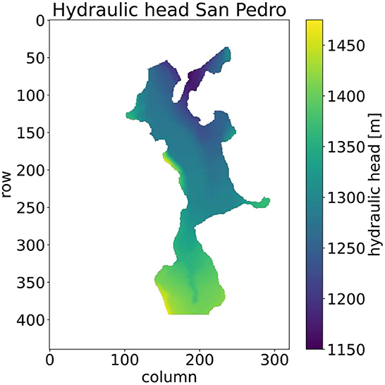
Figure 1. Hydraulic head map of the San Pedro River Basin groundwater model.

2.4.1. Input features and training data set

The selection of a few, influencing input features (feature space A) is important for the simplicity of the network and its ability to understand the problem. Here, both static features (features that do not depend on well location) and location-dependent features (features that depend on the location of the well) are of interest. In a given model cell the static features do not change as the well location is moved, while the location-dependent features do change. Hydraulic conductivity (and the logarithmic conductivity) and hydraulic head prior to pumping are considered important static features, with clear connections to changes in hydraulic head (Garcia and Shigidi, 2006; Chen et al., 2020). If objects such as large rivers are present, the distance to them is also selected as a feature. For the location-dependent features, it is expected that the distance to the well is an important feature with a high correlation to the target feature. The travel time of the water to the well is also considered an important input feature. The feature is approximated as a scaled velocity field estimated using the fast-marching method from scikit-fmm (Furtney, 2021). Input features for the MLP-NN are taken from the individual grid cells in the model as a vector format of size 1 × 9 including the randomly drawn pumping rate and well location. Therefore, a single well simulation generates thousands of input vectors. The input features of a single well simulation in the San Pedro River Basin model are shown in Figure 2 in a 2D grid format, here without pumping rate and well location. Distance from the well and travel time are shown for a well located in cell [185,175]. This selection of input features is based on general availability in MODFLOW models, connection to changes in hydraulic head, modeling choices, and performance in training and testing of the network. Features should be available in most MODFLOW models to generalize the training process. In this way, the setup can be applied to new models with few modifications. All features should have a connection to change in head as this is expected to improve training. Too many random input features might prevent the network from learning the relationship to changes in head. Features should represent the modeling choices made. These are well location (row and column number) and pumping rate.

FIGURE 2

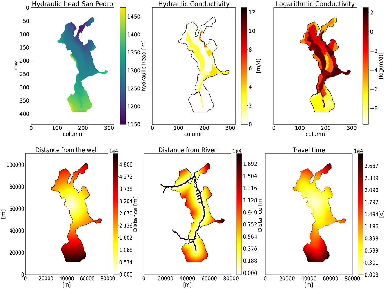
Figure 2. The input features except pumping rate and well location for the MLP-NN in the San Pedro River Basin model. Distance from the well and travel time changes as the well is moved while the other features are static, meaning that they do not change as the well is relocated. Here shown with a well located in row 185 and column 175.

Most of the target data set consists of hydraulic head changes close to zero because of large distances to the well. This uneven distribution of observations might prevent the network from learning the effects of the well both close to and far away. The data is therefore binned according to the head change values and a data subset is constructed by sampling from these bins so that the observations are evenly distributed. Prior to training, the data subset is randomly split into training, testing, and validation data sets (Pedregosa et al., 2011). Here, 20% of the set is allocated to the test set and new random simulations, not included in training or test sets, are used for the validation set (Raschka, 2018). In this way, all sets contain random data from random well simulations of the groundwater model.

To summarize the data set construction, we:

• perform 1,000 steady-state simulations of wells at random locations with variable pumping rates and save the head change in each cell from all simulations. These changes are the target data.

• Construct vectors of input features (features in Figure 2, pumping rate, and well location) that match the target data. One input vector of size 9 × 1 per target data for training.

• Sample from these vectors of input features and target data to construct a data subset that contains an even distribution of observed head changes. This makes the data construction [A, D] as described in Section 2.2.

• Split the data subset 80/20 into a training set and a test set. A third data set from new, independent simulations are used for validation after training.

The full work process is illustrated in Figure 3.

FIGURE 3

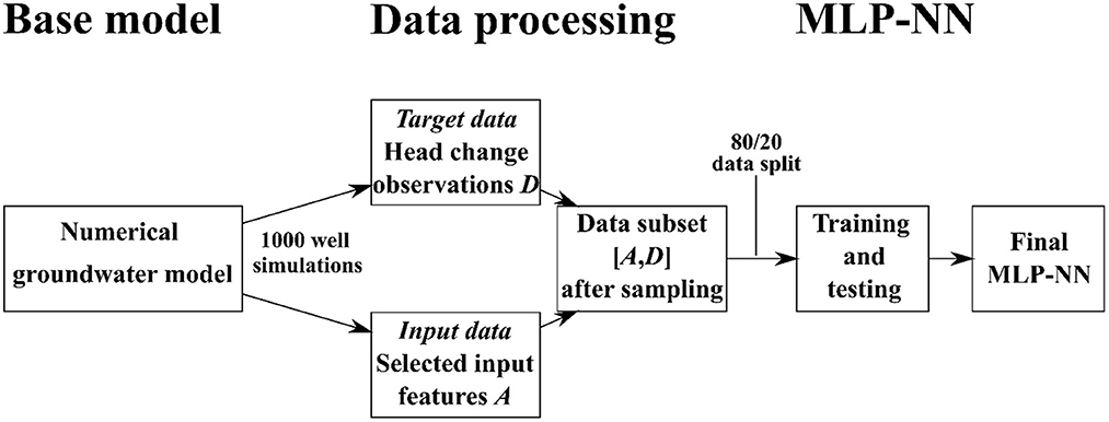
Figure 3. Road map illustrating the process between going from the base groundwater model to the final, trained MLP-NN.

2.4.2. Designing and training the MLP-NN

TensorFlow v2.3 (Abadi et al., 2016) is used for the task of constructing and training the MLP-NN. As discussed previously the input layer is configured with a number of neurons equaling the number of training input features for the considered model (Table 1), and the output layer consist of two neurons representing the mean and standard deviation of a 1D normal distribution representing the change in head value. The loss function, equation (6), is implemented using the Tensorflow probability package (Dillon et al., 2017).¹

TABLE 1

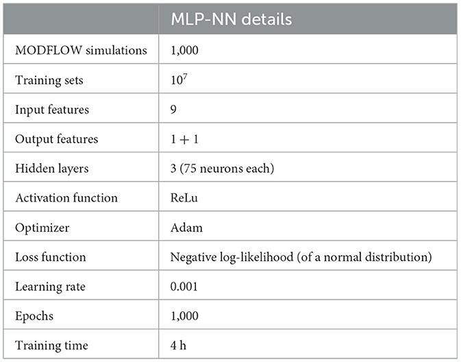
Table 1. Configuration and training details on the multilayer perceptron.

The training data set is used to train the model, while the test and validation data sets are withheld from training. The test set is used to give an unbiased evaluation of the model while training. This is usually referred to as the train-test split approach for model evaluation. The combination of training and evaluation with the train-test sets is used for hyperparameter optimization and helps prevent over-fitting of the network (Cawley and Talbot, 2010). However, the use of the test set multiple times for hyperparameter optimization might introduce a bias and affect the generalization performance of the network. Therefore, a third and independent validation set is used to evaluate the final model (Raschka, 2018).

We manually examine loss curves and validation set performance for networks with varying hidden layer sizes, number of neurons, and activation functions. This is also referred to as a trial and error method. More structured and exhaustive optimization methods are presented and discussed in Yang and Shami (2020). The selected network hyperparameters in Table 1 are the results of this manual search with a focus on minimizing loss, a simple network structure, and minimal overfitting. The hidden layers consists of 3 layers with 75 neurons each (Figure 4) using the ReLU activation function (Nair and Hinton, 2010; Schmidhuber, 2015). A linear activation function transforms the inputs from the third hidden layer to the output layer. Additional information on the configuration and training time of the MLP-NN is further listed in Table 1.

FIGURE 4

Figure 4. The structure of the multilayer perceptron. The input layer takes in a number of input features A (Table 1) and connects them to the three fully connected hidden layers with 75 neurons each. The mean value u and the standard deviation σ of the outcome distribution are estimated in the output layer.

3. Results

We test the MLP-NN's abilities to predict hydraulic head changes from groundwater abstraction in the San Pedro groundwater model and compare the results to MODFLOW simulations. The MLP-NN is also applied in an experimental set-up, where the pumping rates of a well system are varied. The same set-up is solved using the RM approach and MODFLOW for comparison in computation time and accuracy.

3.1. Comparison to MODFLOW

As a test, the MLP-NN is used to simulate the hydraulic head change caused by a well abstracting groundwater in cell [185,190] in the fourth layer of the San Pedro groundwater model. The simulation requires the input features, A, corresponding to the well set-up and the trained network, g_nn, to link these to the hydraulic head change output distribution. The mean values of the predicted normal distributions from the MLP-NN are visualized in Figure 5 along with the results from simulations using MODFLOW in the same set-up. Figures 5A, B, show the hydraulic head change from a well with pumping rate $Q_1=1000\frac{m^3}{d}$ computed with MODFLOW and the MLP-NN, respectively. Figures 5E, F show the change from a pumping rate of $Q_2=2000\frac{m^3}{d}$. Noticeably, the MLP-NN seems to capture both strength in head change and the spatial extent of change in the model when comparing it to the considered true MODFLOW model. It, furthermore, compares well to MODFLOW when increasing the pumping rate from Q₁ to Q₂. Standard deviations on the MLP-NN predictions are shown in Figures 5C, G. Mean head change predictions are subtracted from the MODFLOW results in Figures 5D, H for the two different pumping rates. The mean absolute errors between MODFLOW and the MLP-NN are mae_Q1 = 0.010 m and mae_Q2 = 0.015 m.

FIGURE 5

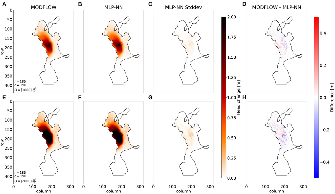
Figure 5. Hydraulic head changes from a simulated well in cell [185, 190] in the test case model. (A, E) MODFLOW simulations with pumping rate ${\text{Q}}_1=1000\frac{{\text{m}}^3}{\text{d}}$ and ${\text{Q}}_2=2000\frac{{\text{m}}^3}{\text{d}}$, respectively. (B, F) MLP-NN mean predictions with pumping rates Q₁ and Q₂, respectively. (C, G): MLP-NN standard deviations. (D, H): Difference between MODFLOW results and MLP-NN predictions.

Since the MLP-NN predicts a normal distribution of outcomes it is possible to evaluate on the accuracy of the network by checking how many MODFLOW observations lie within the 95%-confidence interval of the predicted distribution. In the scenario with pumping rate Q₁, 94.6 % of the MODFLOW head change observations (Figure 5A) lie within the 95%-confidence interval of the corresponding predicted distributions from the MLP-NN (Figure 5B). In the second scenario with pumping rate Q₂, 95.6% of the observations (Figure 5E) are within the 95%-confidence interval of the MLP-NN predictions (Figure 5F). The results show that the MLP-NN is capable of replicating the MODFLOW results within the estimated uncertainty band.

3.2. Comparison to the response matrix case A

For comparison with the RM, two experimental well systems are constructed and response matrices are built to represent these systems. After building the matrices, head change can be estimated from varying pumping rates without running MODFLOW again.

The first set-up consists of three active wells to simulate a multi well-system around the same area as Figure 5 in cells [182, 177], [185, 190], and [190, 188]. The head changes in the model from each of the wells with pumping rates of $Q=1000\frac{m^3}{d}$ are simulated using MODFLOW and used to build the RM following equation (3). Head change from each well is also predicted using the MLP-NN and summed up for a total hydraulic head change caused by the well system. The results from MODFLOW, the RM, and the MLP-NN are shown in Figures 6A–C. Here the results from MODFLOW (Figure 6A) and the results from the RM approach (Figure 6B) are similar since the MODFLOW results are used as a reference to calculate the response coefficients [Equation (3)]. The pumping rate of all wells is then increased to $Q=4000\frac{m^3}{d}$ and the total hydraulic head change is estimated using the same three methods in Figures 6D–F. This time, the already built RM is used to connect the increase in pumping rates to the change in hydraulic head by solving the linear relationship in Equation (3). In the MODFLOW example (Figure 6D) the code is rerun with the new pumping rates of each well, and for the MLP-NN new predictions are made with the change in pumping rates noted in the input features (Figure 6F).

FIGURE 6

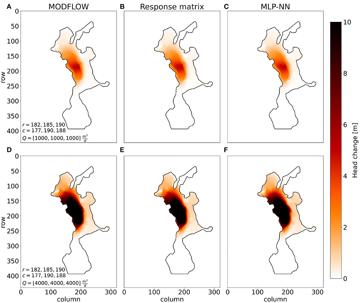
Figure 6. An experimental set-up of three active wells in two scenarios with different pumping rates, where the head changes are computed using MODFLOW, the response matrix approach, and the trained MLP-NN. (A–C) Computed head changes with the three methods where $\text{Q}=1000\frac{{\text{m}}^3}{\text{d}}$ for all wells. (D–F) Computed head changes with the three methods where the pumping rate is increased to $\text{Q}=4000\frac{{\text{m}}^3}{\text{d}}$ for all wells. r and c are the row and column locations of the wells.

By comparing the RM and MLP-NN results to the considered truth from the MODFLOW results (Figures 6A, D) we observe that both two alternative methods provide good results, for both low (Figures 6B, C) and high pumping rates (Figures 6E, F). Mean absolute errors for the response matrix method are mae_{resp_1000} = 0 m and mae_{resp_4000} = 2.74 m, while the mean absolute errors for the MLP-NN are mae_{MLP_1000} = 0.02 m and mae_{MLP_4000} = 2.78 m. This small difference indicates that the change in hydraulic head from increasing the pumping rates of the well-system is a linear relationship.

3.3. Comparison to the response matrix case B

In the second set-up, a single well is placed in [305, 180] with a pumping rate of $Q=1000\frac{m^3}{d}$. Once again the results from MODFLOW are used to estimate the response coefficients for the RM approach. Results using MODFLOW, the RM approach, and the MLP-NN are shown in Figures 7A–C along with the standard deviation on the predictions from the MLP-NN (Figure 7D). The pumping rate is later increased to $Q=5000\frac{m^3}{d}$ and hydraulic head changes are calculated again (Figures 7E–H). From the MODFLOW results (Figures 7A, E), we observe a significant difference in the head change as the pumping rate is increased. A second area around cell [250, 200] in the model experiences high head change and the affected area from the increased groundwater abstraction is significantly increased. This effect is a consequence of the numerical model set-up, where a threshold pumping rate is exceeded and water is abstracted from the upper layers. These upper layers have no-flow cells in the rows and columns near the well causing the model to abstract water from nearest active cells around cell [250, 200] resulting in a second area of high head change in all layers. This non-linear effect in the MODFLOW results is not detected with the RM approach (Figures 7B, F) because of the assumption of linearity. The RM method has some success in replicating the MODFLOW results close to the well, but underestimates the change in head in a large part of the model. This is not the case with the MLP-NN (Figures 7C, G) which can reproduce the non-linear effect in the MODFLOW results. The MLP-NN predicts the extent of the change well, but slightly underestimates the strength of change in the area around cell [250, 200]. However, the standard deviation map (Figure 7H) shows that the MLP-NN is more uncertain in the predicted change in this area correlating nicely with the underestimation of change. The mean absolute errors for the response matrix are mae_{resp_1000} = 0 m and mae_{resp_5000} = 0.085 m, while the mean absolute errors for the MLP-NN are mae_{MLP_1000} = 0.004 m and mae_{MLP_5000} = 0.033 m. For this, more difficult case the MLP-NN provides an efficient alternative to MODFLOW, whereas the use of the RM can be very problematic to use for decision making, due to the ignoring of non-linear effects. This is also confirmed by the mean absolute errors, where the response matrix error is almost three times higher than the MLP-NN.

FIGURE 7

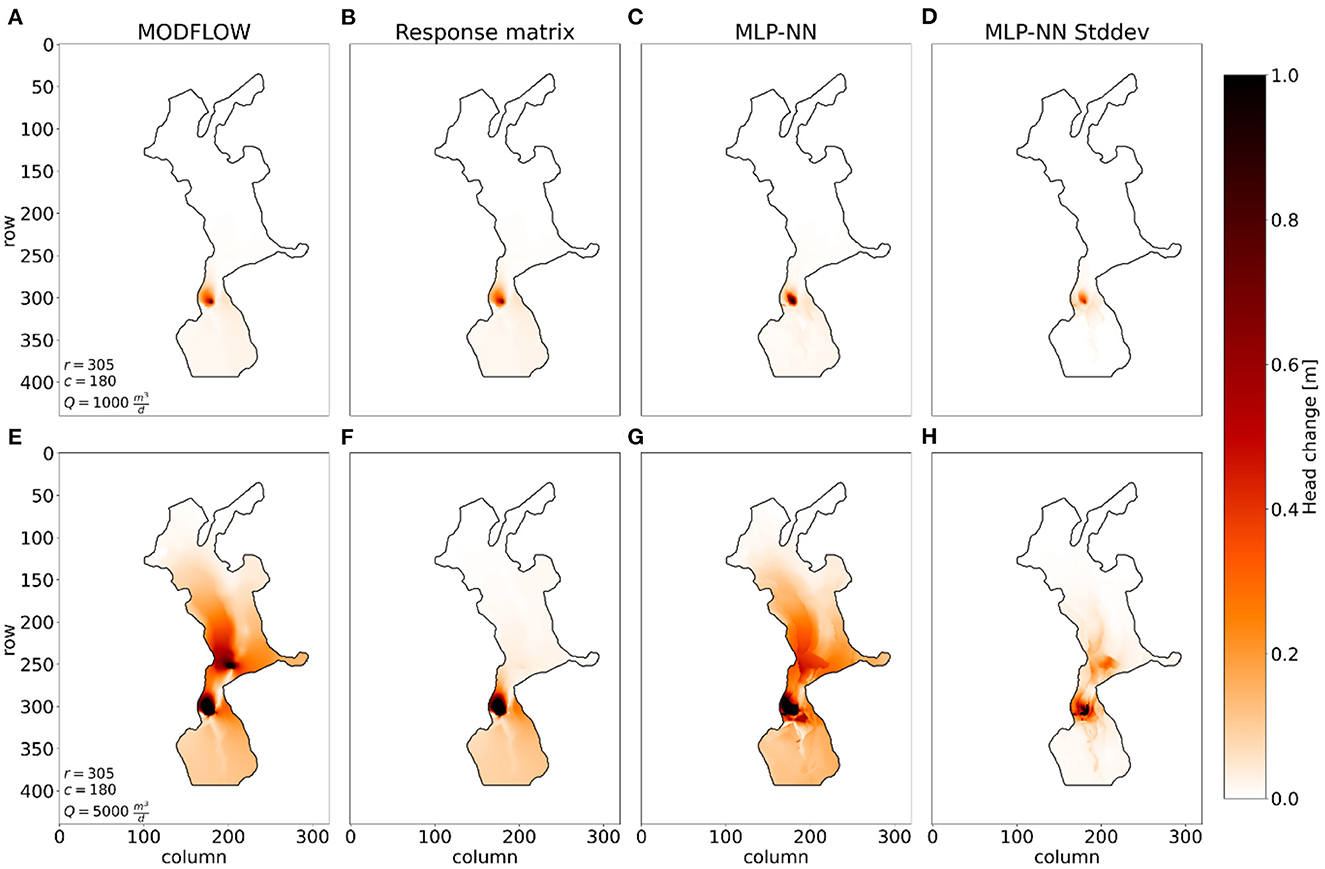
Figure 7. An experimental set-up of an active well in two scenarios with different pumping rates, where the head changes are computed using MODFLOW, the response matrix approach, and the trained MLP-NN. (A–D) Computed head changes with the three methods where $\text{Q}=1000\frac{{\text{m}}^3}{\text{d}}$. (E–H) Computed head changes with the three methods where the pumping rate is increased to $\text{Q}=5000\frac{{\text{m}}^3}{\text{d}}$. r and c are the row and column location of the well.

3.4. Non-linear head change

The non-linear abilities of the MLP-NN is further exploited in Figure 8, where the relationship between head change and pumping rate is investigated in a single observation cell using the same well set-up as in Figure 7. Here, the estimated head change in cell [250, 190] is plotted for increasing pumping rates. The red line is the calculated head change from MODFLOW that looks piece-wise linear with a breaking point around a pumping rate of $2800\frac{m^3}{d}$. The dashed blue line is the RM that continues to estimate head change as the first linear part of the MODFLOW line with no breakpoint. This means that the method works well up to a certain pumping rate and then starts to underestimate the head change in the observation point.

FIGURE 8

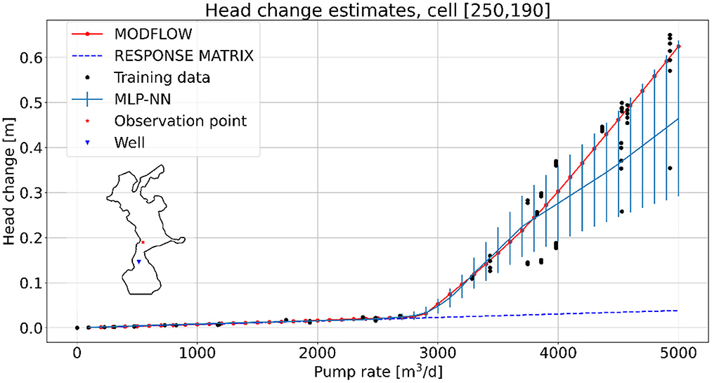
Figure 8. Head change as a function of pumping rate in observation point [250, 190] (red dot) from an activate well in [305, 180] (blue triangle). The relationship is estimated using MODFLOW (red line), the response matrix approach (blue dashed line), and the MLP-NN (light blue line with error bars, one standard deviation). Included are also the training data observations (black dots) with input feature vectors close to the input features for the observation point.

The light blue line with error bars is the MLP-NN's predictions of head changes with one standard deviation. It shows a similar piece-wise linear relationship as MODFLOW and correctly identifies the breakpoint. At around $3900\frac{m^3}{d}$ the MLP-NN line starts to deviate from the MODFLOW line resulting in underestimated mean head changes. However, this deviation correlates well with an increase in uncertainty on the predictions and all MODFLOW observations are within one standard deviation of the MLP-NN results.

The black dots show head changes of input feature vectors with values close to the input feature vector of the observation point. Features are selected by searching for distances to well, time, and distance to river within 5 percent of the standard deviation of the features in the whole training data set. Initial head values are within 10 percent of the standard deviation to get enough observations. The responses from the selected feature vectors show almost no spread before the change in linearity. Afterward, the spread in responses increases around the MLP-NN line together with the increasing standard deviation of the MLP-NN predictions.

The black dots in Figure 8, is representative of examples of different data responses one could get by evaluating the g_A(A) in Equation (4), using only data in the training data set. As discussed in Section 2.2, g_A represent a non-unique mapping, as can be seen by the black dots representing data from the training data set. It is exactly this spread of data, that the MLP-NN is designed to estimate. The uncertainty estimates (blue vertical lines) in Figure 8 suggest that the estimated uncertainty using g_nn corresponds well to the uncertainty given the use of the feature space, in g_A. This is also supported by the confidence interval analysis provided in Section 3.1.

3.5. Network output and speed

We use the 50 simulation runs from Figure 8 to give an estimate of the speed up between MODFLOW and the MLP-NN. The mean runtime including one standard deviation of a MODFLOW simulation in the San Pedro model is t_mod = 24.78 ± 0.78 s. The mean prediction time of an MLP-NN simulation including running the fast marching algorithm for input feature creation is t_MLP = 0.19 ± 0.01 s. Nearly 85% of this time is dedicated to the fast-marching algorithm and the rest to the prediction time. This gives an estimated speed up when using the MLP-NN of 130.1 ± 6.2 times faster than MODFLOW. The fast prediction time and high accuracy make the MLP-NN a feasible option in a decision support framework.

4. Discussion

In this paper, we have implemented a Multilayer Perceptron Neural Network to estimate the hydraulic head change from groundwater abstraction in a numerical groundwater model. The MLP-NN was trained with responses from a MODFLOW groundwater model as target data together with local hydrological attributes and spatial information as input features. The architecture of the MLP-NN was constructed to predict a distribution with a mean and standard deviation instead of a single value in the output layer. The performance of the MLP-NN was tested against MODFLOW and the alternative RM approach in different experimental well system set-ups to investigate the relevance of the MLP-NN in a decision support framework.

The drawdown predictions using the MLP-NN are comparable to the MODFLOW simulations for different pumping rates. Moreover, the estimated uncertainty on the predictions are consistent with the magnitude of the actual errors between the MLP-NN and MODFLOW simulations (Figure 8). This gives the MLP-NN an advantage compared to the RM approach, as it is possible to address the trustworthiness of the prediction using the standard deviation of the predicted distribution. Furthermore, the MLP-NN predictions proves to be on average 130 times faster than MODFLOW for the problems presented, making the network a better alternative in a decision support framework, where scenario analysis and speed are key properties.

Examples are presented (Figures 6, 7) where the MLP-NN are compared the RM method. The results of the first scenario (Figure 6) are very similar for both MODFLOW, the RM, and the MLP-NN, as also revealed by the similar and low mean absolute errors (MAE). In this case, it can be argued, that constructing and training an MLP-NN is redundant since it is essentially solving a linear problem that can easily be solved using the RM. However, the MLP-NN is, unlike a constructed RM, not only applicable to a specific well system set-up. In the second scenario (Figure 7), a new RM is constructed from a MODFLOW simulation, while the existing MLP-NN can be readily applied. In this scenario, the RM underestimates the hydraulic head change for high pumping rates due to a non-linearity in the groundwater model response (Figures 7E, 8). The non-linearity is well resolved with the MLP-NN and predicted head changes are similar to MODFLOW calculations. This translates into a significant difference in MAE. The ability to resolve non-linearity, consistent within the estimated uncertainty range, is the primary advantage of our trained MLP-NN compared to the RM approach. This is especially seen in Figure 8, where the error for both methods increases for higher pumping rates, but MODFLOW results are still within the predict range of the MLP-NN. In more complex groundwater models the risk of getting non-linear responses increases rendering the RM method less applicable. Moreover, since the RM approach does not estimate predictive uncertainty, such non-linearities will remain unknown, potentially resulting in biased decisions. The speed and accuracy of the MLP-NN make it valuable in decision-making for problems where many possible scenarios are considered. Simulating all scenarios in MODFLOW is often not feasible within the asserted timeframe and better management decisions might be overlooked. The MLP-NN can in such cases act as an approximative screening tool that quickly identifies which scenarios are worth further investigating and which are likely to fail. The MLP-NN could also function in a decision support tool as a warning system that alarms users in the case of non-linearities. A decision support tool acting on results from an RM is fast, but limited to the near-linear regime for accurate calculations. Deviations from linearity are difficult to detect without running the MODFLOW model, thereby losing the effect of the RM. With the MLP-NN's understanding of non-linear responses (Figure 8), a fast comparison of results from the RM and the MLP-NN could be performed to check for linear deviation. If results are noticeably different, the decision support tool could issue a warning.

This research shows that the MLP-NN can function in both linear and non-linear domains and only needs to be trained once to work in a wide range of well system set-ups. The MLP-NN is in this way very flexible but should still be limited to the groundwater model and range of simulations, it is trained from. This limitation ensures that the network is not extrapolating to predict results from input features outside the trained range. A network trained on one groundwater flow model could not be applied to predict on a different model setup without extrapolating. However, the simplicity of the chosen input features and straightforward construction of training data ensure that the process of training the MLP-NN using another groundwater model can be done with only a few considerations and modifications to the presented method. In a decision support framework, we would require one trained MLP-NN per groundwater model, and it would be responsible to introduce a limit on e.g., the maximum pumping rate so that it matches the value from the training set. Future work could focus on evaluating the transferability (Bjerre et al., 2022) of the MLP-NN to outside the trained area and use this information to develop networks with increased flexibility to further reduce the limitations of this study.

Future work could also compare the MLP-NN to other types of regression methods. There may exist other methods that can outperform the MLP-NN in accuracy and with less uncertainty. This type of “best fit” exercise has been performed in multiple studies for a wide range of problems (Barzegar et al., 2017; Sahoo et al., 2017; Knoll et al., 2019; Sameen et al., 2019; Najafzadeh and Niazmardi, 2021). Such comparison is left to future work as it is expected not to add much scientific value and might take away the focus of this paper. We argue that the real value of our work is in the input feature selection and the probabilistic output of the MLP-NN. The development of Tensorflow (Abadi et al., 2016) and Scikit-learn (Pedregosa et al., 2011) has made it easier to implement many types of machine learning methods. Together with this work's available code repository, such a comparison should be feasible to perform for the interested reader.

The presented approach distinguishes itself from earlier studies in especially two main ways. Firstly, our trained MLP-NN offers a high degree of flexibility by the user, not considered in earlier studies replacing traditional numerical groundwater models with neural networks (Chu and Chang, 2009; Chen et al., 2013). The MLP-NN is neither bound to a specific well system configuration nor to a constant pumping rate. Secondly, predicting head changes as distributions instead of single values with a neural network is, to our knowledge, unique to this study. Neural networks have been used to accelerate uncertainty estimates in groundwater modeling (Lykkegaard et al., 2021), but not as direct outputs of the network.

We have presented a network which is trained using responses from a numerical model and which estimates prediction uncertainty. As discussed in Section 2.2. this uncertainty is related to using the specific choice of low-dimensional feature space, leading to an implicit ideal forward model g_A, that is non-unique, in that the same set of features, can lead to different change in head. Figure 8 suggests that the trained MLP-NN, g_nn, provides results consistent with g_A. This suggest that g_nn mimics g_A well. It also suggests that other choices of neural network architecture, should not lead to substantially different results, but could well lead to more efficient training. Instead, if one would like to reduce the uncertainty of the predictions using network g_nn, and hence g_A, then one should focus on finding a feature data A that represent the model parameters M, even better than in the case, we present here.

The presented results rely on the existence of a deterministic groundwater model, i.e., without any uncertainty regarding the hydrological model parameters. If a stochastic groundwater model is available, from which multiple hydrological models can be realized, such uncertainty could potentially, and straightforwardly, be used by the proposed methodology. Multiple simulations, based on different groundwater model realizations, with the same well location and pumping rate would result in a distribution of outcomes from the MODFLOW model that, applying the methodology of this paper, could be used in a training data set to represent the uncertainty from varying model parameters. The training data set and time spent to train the MLP-NN would increase, but the trained MLP-NN would predict with the same speed as before since no architectural changes are made. This also means that the MLP-NN has the potential to become even faster than MODFLOW, which would now have to be run multiple times to obtain a distribution of possible outcomes instead of just ones.

Table 2 sums up the results from the comparison of the three methods. Here results obtained using MODFLOW are considered the optimal solution. Since the MLP-NN is trained using simulations from MODFLOW, the accuracy of the MLP-NN cannot outperform the underlying numerical model and remains an approximative approach that, in the presented cases, performs with high accuracy and speed. The MLP-NN's ability to resolve non-linear problems is a clear advantage over the presented RM and shows that it is a better approximative method as a decision support tool in the presented case. The methods' feasibility in decision support (Table 2) is based on their speed and ability to present accurate results in both linear and non-linear cases. As MODFLOW simulations can take a long time to run, it is not suited as a decision support tool for users requiring fast solutions. The RM is very fast but constrained to linear approximations. Therefore, its application in decision support is feasible but limited. The MLP-NN is not constrained by linear assumptions, predicts with high accuracy, and has a high computational speed. In this sense, decision support is feasible once training of the MLP-NN is complete. The distribution output format and uncertainty estimate presents some future opportunities of including uncertainties from the actual numerical model in the network predictions. Following the same approach as presented in this paper, training such a network would require more numerical simulations and training time, but after training, the network is expected to perform just as fast as before and now much faster than the stochastic numerical model. The MLP-NN approach functions as a replacement for the RM method especially for non-linear problems, and outperforms the RM approach by estimating prediction uncertainties and thereby validity of the approximative solution.

TABLE 2

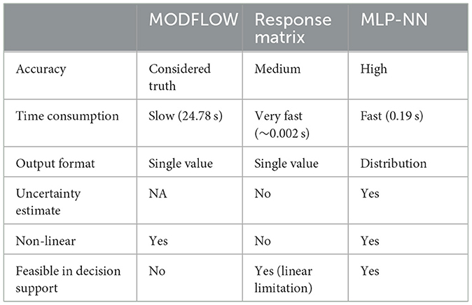
Table 2. Abilities of the three simulation methods.

5. Conclusion

This paper presents a method of training a Multilayer Perceptron Neural Network to predict hydraulic head change from groundwater abstraction using only a few, selected input features. The high accuracy and speed makes it a valuable methodology in a decision support tool framework, where forward runtime is important and approximate calculations are sufficient. With an experimental well system set-up, we show that the MLP-NN can reproduce non-linear responses that the RM method fails to resolve, and that it, once trained, is more flexible to changes in the location of well-systems. The architecture of the MLP-NN is designed to output a normal probability distribution, with a mean and standard deviation per prediction. This allows estimation of the uncertainty in the forward model due to the use of a low-dimensional feature space. The standard deviation shows increasing uncertainty when prediction error increase, indicating that it could be a good measure of prediction trustworthiness. The uncertainties estimated in the present study are a measure of the MLP-NN to reproduce the original model.

Data availability statement

The work is available at zenodo doi: 10.5281/zenodo.7711227. The data used in this study for the San Pedro groundwater model can be accessed at doi: 10.1111/gwat.12413.

Author contributions

MD: conceptualization, methodology, software, formal analysis, writing—original draft, writing—review and editing, and visualization. TV: conceptualization, methodology, writing—review and editing, and supervision. TB: conceptualization, writing—review and editing, supervision, and project administration. TH: conceptualization, methodology, writing—review and editing, supervision, and project administration. All authors contributed to the article and approved the submitted version.

Funding

This work is funded by the Innovation Fund Denmark, project 9065-00212B.

Acknowledgments

A special thanks to Mads Paulsen and Adrian Barfod for great conversations on machine learning and Python.

Conflict of interest

TV and MD were employed by NIRAS.

The remaining authors declare that the research was conducted in the absence of any commercial or financial relationships that could be construed as a potential conflict of interest.

Publisher's note

All claims expressed in this article are solely those of the authors and do not necessarily represent those of their affiliated organizations, or those of the publisher, the editors and the reviewers. Any product that may be evaluated in this article, or claim that may be made by its manufacturer, is not guaranteed or endorsed by the publisher.

Footnotes

1. ^Python code available on GitHub https://github.com/MathiasBusk/HYDROsimpaper. Training data set at Zenodo: https://doi.org/10.5281/zenodo.6817606.

References

Abadi, M., Agarwal, A., Barham, P., Brevdo, E., Chen, Z., Citro, C., et al. (2016). Tensorflow: Large-scale machine learning on heterogeneous distributed systems. arXiv preprint arXiv:1603.04467.

Google Scholar

Bakker, M., Post, V., Langevin, C. D., Hughes, J. D., White, J. T., Starn, J. J., et al. (2016). Scripting MODFLOW model development using Python and FloPy. Groundwater. 54, 733–739. doi: 10.1111/gwat.12413

PubMed Abstract | CrossRef Full Text | Google Scholar

Barzegar, R., Asghari Moghaddam, A., Adamowski, J., and Fijani, E. (2017). Comparison of machine learning models for predicting fluoride contamination in groundwater. Stochastic Environ. Res. Risk Assess. 31, 2705–2718. doi: 10.1007/s00477-016-1338-z

CrossRef Full Text | Google Scholar

Bjerre, E., Fienen, M. N., Schneider, R., Koch, J., and Højberg, A. L. (2022). Assessing spatial transferability of a random forest metamodel for predicting drainage fraction. J. Hydrol 612, 128177. doi: 10.1016/j.jhydrol.2022.128177

CrossRef Full Text | Google Scholar

Cawley, G. C., and Talbot, N. L. C. (2010). On over-fitting in model selection and subsequent selection bias in performance evaluation. J. Mach. Learn. Res. 11, 2079–2107.

PubMed Abstract | Google Scholar

Chen, C., He, W., Zhou, H., Xue, Y., and Zhu, M. (2020). A comparative study among machine learning and numerical models for simulating groundwater dynamics in the Heihe River Basin, northwestern China. Sci. Rep. 10, 1–3. doi: 10.1038/s41598-020-60698-9

PubMed Abstract | CrossRef Full Text | Google Scholar

Chen, Y. W., Chang, L. C., Huang, C. W., and Chu, H. J. (2013). Applying genetic algorithm and neural network to the conjunctive use of surface and subsurface water. Water Resour. Manage. 27, 4731–4757. doi: 10.1007/s11269-013-0418-9

CrossRef Full Text | Google Scholar

Cheng, T., Mo, Z., and Shao, J. (2014). Accelerating groundwater flow simulation in MODFLOW using JASMIN-based parallel computing. Groundwater. 52, 194–205. doi: 10.1111/gwat.12047

PubMed Abstract | CrossRef Full Text | Google Scholar

Chu, H.-J., and Chang, L.-C. (2009). Optimal control algorithm and neural network for dynamic groundwater management. Hydrol. Proces. 23, 2765–2773. doi: 10.1002/hyp.7374

CrossRef Full Text | Google Scholar

Coppola, E., Szidarovszky, F., Poulton, M., and Charles, E. (2003). Artificial neural network approach for predicting transient water levels in a multilayered groundwater system under variable state, pumping, and climate conditions. J. Hydrol. Eng. 8, 348–360. doi: 10.1061/(ASCE)1084-0699(2003)8:6(348)

CrossRef Full Text | Google Scholar

Dagasan, Y., Juda, P., and Renard, P. (2020). Using generative adversarial networks as a fast forward operator for hydrogeological inverse problems. Groundwater. 58, 938–950. doi: 10.1111/gwat.13005

PubMed Abstract | CrossRef Full Text | Google Scholar

Dillon, J. V., Langmore, I., Tran, D., Brevdo, E., Vasudevan, S., Moore, D., et al. (2017). Tensorflow distributions. arXiv preprint arXiv:1711.10604.

Google Scholar

Furtney, J. (2021). scikit-fmm: the fast marching method for Python. Available online at: https://github.com/scikit-fmm/scikit-fmm (accessed August 26, 2022).

Garcia, L. A., and Shigidi, A. (2006). Using neural networks for parameter estimation in ground water. J. Hydrol. 318, 215–231. doi: 10.1016/j.jhydrol.2005.05.028

CrossRef Full Text | Google Scholar

Gardner, M. W., and Dorling, S. R. (1998). Artificial neural networks (the multilayer perceptron) - a review of applications in the atmospheric sciences. Atmosphere. Environ. 32, 2627–2636. doi: 10.1016/S1352-2310(97)00447-0

CrossRef Full Text | Google Scholar

Gorelick, S. M. (1983). A review of distributed parameter groundwater management modeling methods. Water Resour. Res. 19, 305–319. doi: 10.1029/WR019i002p00305

CrossRef Full Text | Google Scholar

Hadded, R., Nouiri, I., Alshihabi, O., Mamann, J., Huber, M., Laghouane, A., et al. (2013). A decision support system to manage the groundwater of the zeuss koutine aquifer using the WEAP-MODFLOW framework. Water Resour. Manage. 27, 1981–2000. doi: 10.1007/s11269-013-0266-7

CrossRef Full Text | Google Scholar

Harbaugh, A. W. (2005). MODFLOW-2005, The U.S. Geological Survey Modular Ground-Water Model — The Ground-Water Flow Process. Reston, VA, USA: U.S. Geological Survey Techniques and Methods 6-A16 USGS. doi: 10.3133/tm6A16

CrossRef Full Text | Google Scholar

Hornik, K., Stinchcombe, M., and White, H. (1990). Universal approximation of an unknown mapping and its derivatives using multilayer feedforward networks. Neural Netw. 3, 551–560. doi: 10.1016/0893-6080(90)90005-6

CrossRef Full Text | Google Scholar

Knoll, L., Breuer, L., and Bach, M. (2019). Large scale prediction of groundwater nitrate concentrations from spatial data using machine learning. Sci. Total Environ. 668, 1317–1327. doi: 10.1016/j.scitotenv.2019.03.045

PubMed Abstract | CrossRef Full Text | Google Scholar

Leake, S. A., Reeves, H. W., and Dickinson, J. E. (2010). A new capture fraction method to map how pumpage affects surface water flow. Ground Water. 48, 690–700. doi: 10.1111/j.1745-6584.2010.00701.x

PubMed Abstract | CrossRef Full Text | Google Scholar

Lykkegaard, M. B., Dodwell, T. J., and Moxey, D. (2021). Accelerating uncertainty quantification of groundwater flow modelling using a deep neural network proxy. Comput. Methods Appl. Mechan. Eng. 383, 113895. doi: 10.1016/j.cma.2021.113895

CrossRef Full Text | Google Scholar

Maier, H. R., and Dandy, G. C. (2000). Neural networks for the prediction and forecasting of water resources variables: A review of modelling issues and applications. Environ. Modell. Softw. 15, 101–124. doi: 10.1016/S1364-8152(99)00007-9

CrossRef Full Text | Google Scholar

Marais, J., and de Dreuzy, J. R. (2017). Prospective interest of deep learning for hydrological inference. Groundwater 55, 688–692. doi: 10.1111/gwat.12557

PubMed Abstract | CrossRef Full Text | Google Scholar

Mohanty, S., Jha, M. K., Kumar, A., and Panda, D. K. (2013). Comparative evaluation of numerical model and artificial neural network for simulating groundwater flow in Kathajodi-Surua Inter-basin of Odisha, India. J. Hydrol. 495, 38–51. doi: 10.1016/j.jhydrol.2013.04.041

CrossRef Full Text | Google Scholar

Mohebali, B., Tahmassebi, A., Meyer-Baese, A., and Gandomi, A. H. (2019). Probabilistic neural networks: A brief overview of theory, implementation, and application. Handb. Probabil. Models 347–367. doi: 10.1016/B978-0-12-816514-0.00014-X

CrossRef Full Text | Google Scholar

Nair, V., and Hinton, G. E. (2010). “Rectified linear units improve Restricted Boltzmann machines,” in Proceedings of the 27th International Conference on Machine Learning (ICML-10) 807–814.

Google Scholar

Najafzadeh, M., and Niazmardi, S. (2021). A novel multiple-kernel support vector regression algorithm for estimation of water quality parameters. Nat. Resour. Res. 30, 3761–3775. doi: 10.1007/s11053-021-09895-5

CrossRef Full Text | Google Scholar

Niswonger, R. G., Panday, S., and Ibaraki, M. (2011). MODFLOW-NWT, A Newton formulation for MODFLOW-2005. US Geol. Surv. Techn. Methods 6, 44. doi: 10.3133/tm6A37

CrossRef Full Text | Google Scholar

Pedregosa, F., Varoquaux, G., Gramfort, A., Michel, V., Thirion, B., Grisel, O., et al. (2011). Scikit-learn: Machine learning in Python. J. Mach. Learn. Res. 12, 2825–2830. doi: 10.48550/arXiv.1201.0490

CrossRef Full Text | Google Scholar

Psilovikos, A. (2006). Response matrix minimization used in groundwater management with mathematical programming: A case study in a transboundary aquifer in Northern Greece. Water Resour. Manage. 20, 277–290. doi: 10.1007/s11269-006-0324-5

CrossRef Full Text | Google Scholar

Raschka, S. (2018). Model evaluation, model selection, and algorithm selection in machine learning. arXiv preprint arXiv:1811.12808.

Google Scholar

Rogers, L. L., and Dowla, F. U. (1994). Optimization of groundwater remediation using artificial neural networks with parallel solute transport modeling. Water Resour. Res. 30, 457–481. doi: 10.1029/93WR01494

CrossRef Full Text | Google Scholar

Sahoo, S., Russo, T. A., Elliott, J., and Foster, I. (2017). Machine learning algorithms for modeling groundwater level changes in agricultural regions of the U.S. Water Resour. Res. 53, 3878–3895. doi: 10.1002/2016WR019933

CrossRef Full Text | Google Scholar

Sameen, M. I., Pradhan, B., and Lee, S. (2019). Self-learning random forests model for mapping groundwater yield in data-scarce areas. Nat. Resour. Res. 28, 757–775. doi: 10.1007/s11053-018-9416-1

CrossRef Full Text | Google Scholar

Schmidhuber, J. (2015). Deep Learning in neural networks: An overview. Neural Netw. 61, 85–117. doi: 10.1016/j.neunet.2014.09.003

PubMed Abstract | CrossRef Full Text | Google Scholar

Specht, D. F. (1990). Probabilistic neural networks. Neural Netw. 3, 109–118. doi: 10.1016/0893-6080(90)90049-Q

CrossRef Full Text | Google Scholar

Sun, M., and Zheng, C. (1999). Long-term groundwater management by a modflow based dynamic optimization tool. J. Am. Water Resour. Assoc. 35, 99–111. doi: 10.1111/j.1752-1688.1999.tb05455.x

CrossRef Full Text | Google Scholar

Yang, L., and Shami, A. (2020). On hyperparameter optimization of machine learning algorithms: Theory and practice. Neurocomputing. 415, 295–316. doi: 10.1016/j.neucom.2020.07.061

CrossRef Full Text | Google Scholar

Yoon, H., Jun, S. C., Hyun, Y., Bae, G. O., and Lee, K. K. (2011). A comparative study of artificial neural networks and support vector machines for predicting groundwater levels in a coastal aquifer. J. Hydrol. 396, 128–138. doi: 10.1016/j.jhydrol.2010.11.002

CrossRef Full Text | Google Scholar