 Alexis Neven
 Ludovic Schorpp
 Philippe Renard
94% of researchers rate our articles as excellent or good
Learn more about the work of our research integrity team to safeguard the quality of each article we publish.
Find out more
ORIGINAL RESEARCH article
Front. Water, 20 October 2022
Sec. Water and Hydrocomplexity
Volume 4 - 2022 | https://doi.org/10.3389/frwa.2022.989440
This article is part of the Research TopicMultifidelity Modelling for Optimization and Analysis of Subsurface and Surface Water SystemsView all 4 articles
In Quaternary deposits, the characterization of subsurface heterogeneity and its associated uncertainty is critical when dealing with groundwater resource management. The combination of different data types through joint inversion has proven to be an effective way to reduce final model uncertainty. Moreover, it allows the final model to be in agreement with a wider spectrum of data available on site. However, integrating them stochastically through an inversion is very time-consuming and resource expensive, due to the important number of physical simulations needed. The use of multi-fidelity models, by combining low-fidelity inexpensive and less accurate models with high-fidelity expensive and accurate models, allows one to reduce the time needed for inversion to converge. This multiscale logic can be applied for the generation of Quaternary models. Most Quaternary sedimentological models can be considered as geological units (large scale), populated with facies (medium scale), and finally completed by physical parameters (small scale). In this paper, both approaches are combined. A simple and fast time-domain EM 1D geophysical direct problem is used to first constrain a simplified stochastic geologically consistent model, where each stratigraphic unit is considered homogeneous in terms of facies and parameters. The ensemble smoother with multiple data assimilation (ES-MDA) algorithm allows generating an ensemble of plausible subsurface realizations. Fast identification of the large-scale structures is the main point of this step. Once plausible unit models are generated, high-fidelity transient groundwater flow models are incorporated. The low-fidelity models are populated stochastically with heterogeneous facies and their associated parameter distribution. ES-MDA is also used for this task by directly inferring the property values (hydraulic conductivity and resistivity) from the generated model. To preserve consistency, geophysical and hydrogeological data are inverted jointly. This workflow ensures that the models are geologically consistent and are therefore less subject to artifacts due to localized poor-quality data. It is able to robustly estimate the associated uncertainty with the final model. Finally, due to the simplification of both the direct problem and the geology during the low-fidelity part of the inversion, it greatly reduces the time required to converge to an ensemble of complex models while preserving consistency.
Quaternary aquifers are frequently used for groundwater supply, but due to their high heterogeneity, they are difficult to characterize and model. A possible strategy is to combine geological knowledge, geophysical data, and hydraulic tests. Geophysical methods, especially electromagnetic (EM) ones, are inexpensive and can efficiently help when facing an under-constrained problem (Barfod et al., 2018; Christensen et al., 2017). They are usually sensitive to several petrophysical parameters, such as resistivity, but provide limited information regarding the hydraulic conductivities or the water storage capacity of the underground. Consequently, inverted geophysical models can be integrated into the first steps of the aquifer modeling workflow by delineating the geological structures from a manual interpretation and obtaining a so-called cognitive model (e.g., Høyer et al., 2015). This approach can be combined with stochastic models to populate the main stratigraphic units with lithologies and represent that level of heterogeneity. Furthermore, one can use geophysical inversion results and borehole data to estimate the probability of occurrence of several lithologies (e.g., clay or sand) and use these probabilities as soft information to generate stochastic realizations that are both constrained by some geological reasoning, borehole, and geophysical data (Jørgensen et al., 2015; Carle and Fogg, 2020). This approach ensures consistency with available knowledge, it reproduces accurately the soft information in terms of probability, but nothing ensures that if the final models were used in a forward geophysical model they would reproduce the field measurements. Furthermore, it is likely that the overall uncertainty may be underestimated because it is rare that the aquifer geometry derived from the cognitive model is assumed uncertain.
To ensure consistency, we propose to reverse the methodology described in the previous paragraph and start by constructing a prior geological model that we will then use in geophysical and hydrogeological inversion. Therefore, the first key ingredient of our proposed methodology is the ArchPy hierarchical modeling approach developed recently (Schorpp et al., 2022). ArchPy decomposes the construction of the aquifer model in three main simulation steps: the stratigraphic units, the litho-facies, and the petrophysical parameters. The approach is automated and accounts for a geological concept described in a data structure called a stratigraphic pile as well as borehole data. ArchPy can quickly generate an ensemble of models compatible with the prior geological knowledge of the site. Each model can serve as input to any geophysical forward or hydrogeological model. Comparing the results of the calculated responses to data measured in the field allows one to estimate the likelihood of any proposed model and identify which one corresponds to the maximum a posteriori likelihood and generate realizations representing the posterior uncertainty. This type of Bayesian strategy combining geophysical and hydrogeological data has shown that it can produce consistent models and allowed to reduce the final uncertainty (e.g., Irving and Singha, 2010; Jardani et al., 2013). But these joint inverse problems are often solved using Markov chain Monte Carlo methods and are computationally challenging (Linde and Doetsch, 2016).
Ensemble Smoothers with Multiple Data Assimilation (ES-MDA) have shown to obtain solutions to complex nonlinear inverse problems more efficiently than Ensemble Smoothers (ES) (Emerick and Reynolds, 2013) and faster than Markov Chain Monte-Carlo (MCMC) methods (Juda et al., 2022). The method uses a Monte-Carlo approximation of the Kalman Filter (Kalman, 1960) where the relations between the state variables and the parameters are estimated using an ensemble of models. ES-MDA and PESTPP-IES (White, 2018) are both variants of the Ensemble Smoothers (ES) algorithm proposed by van Leeuwen and Evensen (1996). The key aspect of ES-MDA is to perform iterative ES corrections of the parameters by assimilating the data of the previous iteration, when PESTPP-IES optimizes directly an objective function using a modified form of the Levenberg-Marquardt algorithm. Lam et al. (2020) showed a comparison of different Iterative Ensemble Smoothers, including PESTPP-IES and ES-MDA. It was shown that PESTPP-IES approach outperforms ES-MDA when the ensemble size is relatively small (200 in the study) but that ES-MDA tends to improve with an increase of the ensemble size, while PESTPP-IES does not. ES-MDA has been successfully applied in groundwater studies (Kang et al., 2019; Lam et al., 2020; Xu et al., 2022). One important underlying assumption is that the state variables and parameters are normally distributed (and even multi-Gaussian). If not, one can apply a normal score transform to ensure that the marginal distributions are Gaussian (Zhou et al., 2011).
A recent study by Wang et al. (2022) proposed a hierarchical inversion, where the posterior distribution of global variables including for example hyper-parameters of the geostatistical models are first estimated using a machine learning approach. Following this, an ES algorithm that includes local reduction of dimension is applied to invert the field parameters.
Even if ES-MDA is known to be faster than the MCMC approaches, it can still be computationally heavy because a proper estimation of the covariance matrices used to estimate the Kalman gains requires running a large ensemble of models and, therefore, running a large ensemble of forward geophysical or hydrogeological models. Often, this step is the one that requires most of the computational power. Therefore, there is still a need to devise techniques to accelerate such approaches, and one is to use a multi-fidelity framework. By using a simple surrogate model, one can approximate the forward model and accelerate the inversion (Asher et al., 2015; Dagasan et al., 2020). This idea has been applied, for example, by Zheng et al. (2019), who trained a Gaussian process model to approximate the forward flow problem in a multi-fidelity ES-MDA algorithm.
In this paper, we employ the multi-fidelity principle and ES-MDA but with a different perspective. We do not try to build a surrogate model of the forward model, but instead, we use the fact that the computing times for the geophysical and hydrogeological forward models are very different and that ArchPy provides a hierarchy of levels of representation of the geological heterogeneity. In practice, we invert jointly the multiple data types in the same workflow using ES-MDA in two steps. To ensure that our aquifer models are geologically consistent, they are generated using ArchPy. To accelerate the inversion, we run first a fast low-fidelity ES-MDA inversion to obtain an initial representation of the main geological discontinuities with the fast geophysical forward only. The complete heterogeneous models are then generated from the low-fidelity ones, and used in a second ES-MDA high-fidelity inversion loop including both the geophysical and hydrogeological forward models. The present paper introduces this idea and demonstrates its applicability to two simple 2D synthetic cases of increasing complexity.
In this study, we propose to combine the advantages of a stochastic ES-MDA inversion with a multi-fidelity approach for joint hydrogeophysical inversion. The model is inverted for both hydraulic conductivities and electrical resistivity. In this section, we first introduce the ArchPy modeling approach and its use for our approach for multi-fidelity geological models. We then briefly introduce the ES-MDA algorithm and present the test case used to benchmark our approach.
The first key tool in our methodology is the stochastic hierarchical geological modeling approach named ArchPy and proposed by Schorpp et al. (2022). The method is implemented in an open source python module and is capable of producing both Low-Fidelity (LFM) and High-Fidelity models (HFM). These models are consistent with the prior geological knowledge and capable of integrating geological information in a hierarchical manner. For a complete description of ArchPy capabilities and algorithms, the readers are referred to Schorpp et al. (2022) and to the repository of the code1.
In short, ArchPy relies on the concept of Stratigraphic Pile (SP) which is used to formalize the existing geological knowledge for a given site. All the rules, information, and parameters required to generate the geological models are stored in the SP. For example, the SP contains the list of the stratigraphic units that must be simulated, the list of litho-facies to simulate in which units, and the different simulation parameters (covariance functions, Training images for MPS, etc.). The SP is defined by the user and represents his prior knowledge. Once the SP, is defined ArchPy constructs automatically the models in three main steps:
• The stratigraphic units are first simulated using 2D simulation of the surfaces bounding the units (Figure 1A). The user can select different geostatistical algorithms such as Multiple-point statistics (MPS; Mariethoz et al., 2010) or Sequential Gaussian Simulations (SGS; Deutsch and Journel, 1992). This step handles erosional events where older and previously simulated surfaces are partially eroded by younger ones. It also allows some units not to be deposited (i.e., hiatus). Moreover, inequality data are used to account for incomplete information provided by a borehole that did not reach a certain unit or when there is a hiatus in a stratigraphic sequence.
• The units are then filled with litho-facies (e.g., gravel, silt, clay, etc.) using 3D categorical simulations methods (Figure 1B). Again, the user can chose among MPS or Sequential Indicator Simulation (SIS; Journel, 1983; Journel and Isaaks, 1984). The litho-facies models can be different for every unit and the simulations are conditioned by borehole data if available.
• Finally, the facies are populated by continuous petrophysical properties such as hydraulic conductivities, porosity, or electrical resistivity using SGS (Figures 1C,D). The parameters are defined separately for the different litho-facies.

Figure 1. Two dimensional example of an ArchPy simulation with the three simulation steps. (A) Simulation of units. (B) Simulation of facies. (C) simulation of the resistivity field. (D) Simulation of the permeability field.
An important feature of ArchPy is that the different hierarchical levels only depend on the higher ones (for example, facies only depend on the stratigraphic unit simulations). This feature allows to consider the geological representation of the underground at different level of fidelity.
Finally, ArchPy allows defining stratigraphic sub-units. This option is not used in the present paper but allows simulating complex stratigraphies when needed. By operating as described above, a large number of stochastic simulations can be obtained using ArchPy. They are all conditioned by optional borehole data and geological concept (the stratigraphic pile).
The proposed inversion approach is divided in two main steps: low-fidelity and high-fidelity. The objective of using computationally inexpensive low-fidelity models is to reduce the dimension of the parameter space in which we need to solve the inverse problem with the computationally costly high-fidelity models. Low-fidelity models consist of simplified models. LFMs neglect the small and medium-scale variability of the properties by assuming that the stratigraphic units have a completely homogeneous facies with a unique property value for each unit. The value is drawn from a given uniform distribution in each layer. So, it can vary between the models, but not within one. This step is crucial as it prevents the inversion algorithm from being over-confident, in order to mitigate our assumption that the units are homogeneous. It also allows having a more complete exploration of the parameter space and plausible realizations. The LFMs are generated using the ArchPy package. They correspond to the first hierarchical modeling step (Figure 1A) and are homogeneously filled.
An important aspect to note is that it is not the petrophysical field that is inverted at this stage. The parameters of interest are the altitude of the surface(s) delineating the main stratigraphic units. By doing so, we significantly reduce the number of unknowns while still working on a simplified geologically consistent model. Moreover, LFMs are solely evaluated on the geophysical data, as the geophysical forwards are much faster than the groundwater ones (around 15 times faster).
The high-fidelity models (HFMs) are also generated with ArchPy. These models depend on the LF ones. All the surfaces obtained via the LF inversion step are used to generate the next level of hierarchical simulations (heterogeneous litho-facies and properties). The HFMs are more realistic subsurface models than LFM and are closer to the geological concept. They present heterogeneous facies distributions, with high property contrasts even within a unit (see example on Figures 1C,D). These complete fields will then be inverted. The number of models is not necessarily the same in the two steps (LF and HF). This allows more flexibility, as it is expected that the two problems may not require the same number of models to converge properly. Generally, we expect that we will have more HF than LF models, since the second problem is more difficult and have to integrate more data. Therefore, the same surfaces can be used multiple times and be associated to different facies and parameter distributions.
The general strategy for the multi-fidelity inversion is to employ the same ES-MDA algorithm (Emerick and Reynolds, 2013) successively for the low fidelity and high fidelity geological models (Figure 2) but on different parameters. For the low fidelity, the algorithm will update only the geometry of the surfaces bounding the stratigraphic units, while for the high fidelity models, it will update the complete model including geometry and parameter fields (resistivity and hydraulic conductivities). The two steps are coupled because the ensemble of surfaces obtained from the low fidelity inversion step are used to initialize the generation of the ensemble of high fidelity models used in the second step.
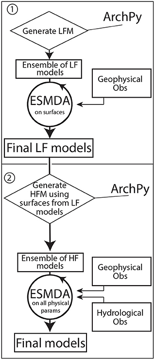
Figure 2. General workflow of our approach. The two main steps are differentiated: one for the low-fidelity part; two for the high-fidelity part.
On both fidelities, the ES-MDA inversion algorithm is applied on a set of N members representing the prior. To ensure that the parameters are multiGaussian, we applied a normal score transform on the prior models (Deutsch, 2002, p. 44–48). This step was not needed when performing the inversion on the low-fidelity models, since the surfaces are generated using Sequential Gaussian Simulation (SGS) and are by definition multiGaussian. The parameters are updated iteratively on the basis of the observations of the state variables to form a new conditional distribution of parameters. Updates are done, for each member i, according to the following equation:
where k is the iteration step, K the Kalman matrix (or Kalman gain), and is the mismatch between the observed measurements and the predictions computed by the forward operator g using the current parameters. In order to stochastically account for the errors in the measurement, is given by
with Cerr being the expected error matrix and zd, i being drawn from a normal distribution. Compared to ES, the data will be assimilated multiple times in ES-MDA. For this reason, it will tend to overestimate the confidence given to the data (Emerick and Reynolds, 2013). To avoid it, a parameter α > 1 is added to inflate the Gaussian noise. Because of that, the parameters covariance reduction will be limited at each iteration. The inflation factor needs to be fixed such as the following condition is satisfied:
where Niter is the number of iterations of ES-MDA. The alpha coefficient was kept unchanged through the iterations, equals to the number of iterations. Emerick (2016) has shown that varying them do not lead to a significant improvement in the convergence of the algorithm. The α factor is applied when calculating the Kalman gain, such as
where is the cross-covariance matrix between the vector of parameters m and the approximated vector of predicted data g(m) for the ensemble. is the autocovariance matrix of the predicted data g(m). LM is the localization matrix. As shown in Anderson (2001), Wen and Chen (2005), and Evensen (2009), with a limited amount of members, fortuitous long-range correlation can happen. It is necessary to filter them out before applying the Kalman update. To do so, the Kalman gain matrix is multiplied element-wise using a localization matrix (Chen and Oliver, 2011). The purpose is to influence only the parameters located within a certain distance from the observation points during the update. The localization matrix has the same size as the Kalman matrix and its values vary between 0 and 1. It was only used in the HF step of the inversion, and was set as a uniform matrix of ones for the hydrogeological observation. We did that since the expected radius of parameters effect on a point was difficult to properly estimate. For the geophysical data, it was calculated using the correlation function proposed by Gaspari and Cohn (1999), with anisotropy in the distance calculation. Figure 3 shows an example of a localization matrix on resistivity parameters for an observation point. Further away is the observation point, weaker will be the contribution of the Kalman gain on the parameter.
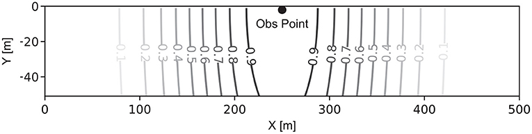
Figure 3. Example of localization matrix LM for one geophysical observation point using a length of 250 m.
To illustrate and test the proposed methodology, we only consider in this paper 2D vertical profiles. Note that the extension to 3D models is straightforward. The domain size is 500 m long for a depth of 50 m, with a cell size of 1 × 1 m. The resulting model consists of 25,000 cells.
Two different cases, C1 and C2, were defined as illustrated in Figure 4:
• Case C1 is the simplest. It considers only two stratigraphic units: one aquifer unit (unit 1) and an aquitard (unit 2). In this situation, the most important feature to identify during the inversion process is the depth of the transition between the two units for each position x.
• The case C2 is more complex, as it includes a possibly discontinuous aquitard with a variable thickness within the main aquifer formation that can be divided into two sub-aquifers. This case can be modeled with four stratigraphic units in ArchPy (see the stratigraphic pile of C2 in Figure 4). The complexity of the problem is increased, as it is now also necessary to estimate, for each location x, the absence or presence of the intermediate aquiclude formation, as well as its depth and thickness in the latter case. A total of three surfaces must be inverted.
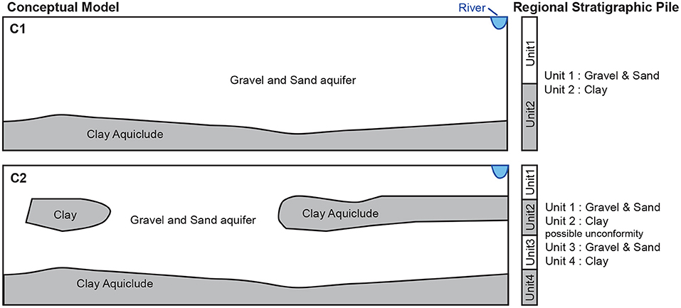
Figure 4. Schematic representation of the geological concepts C1 and C2, with their associated regional stratigraphic pile.
The global conceptual models are inspired from a realistic situation: the Upper Aare Valley in Switzerland. An upper fluvial deposit layer of a few dozen meters overlays a thick lacustrine clay layer. The geological context of the area is briefly described in Schorpp et al. (2022) or Graf and Burkhalter (2016). The upper fluvial deposit may show locally few superficial clay layers. Our synthetic model is a simplified version of this real case. Concerning the geological simulations, for both cases, we assume that no borehole information is available. Thus, all geological simulations are unconditional.
For the low-fidelity models (cases 1 and 2), the surfaces are simulated with SGS and the stratigraphic unit domains are defined. Then, an electrical resistivity value is drawn uniformly between 100 and 400 Ωm in the log space for the aquifers and is taken constant and equal to 10 Ωm for the aquiclude. For cases 1 and 2, we generated an ensemble of 100 LFM to initiate the ES-MDA algorithm. For HFMs, property simulations required two additional steps. The surfaces delimitating the stratigraphic units were taken directly from the ensemble of results of the LFM inversion. The aquifer units (units 1 and 3 in Figure 4) were supposed to be composed only of gravel and sand with a proportion of 70% of gravel and 30% of sand. Sequential Indicator Simulations were used to simulate the position of these facies. The aquiclude units are assumed to be composed only of the clay facies. The different facies are then populated with the desired properties using SGS. The simulation parameters are given in Table 1. For both cases, we generated a total of 500 HFMs based on the 100 optimized LFMs. This implies that there are 500 members for the 2nd step ES-MDA.

Table 1. Geostatistical parameters used by ArchPy to generate the geological models.
During the inversion, two distinct physical forward models are used: one geophysical forward and one hydrogeological forward. The geophysical one is a 1D Time Domain Electro-Magnetic forward. The code used is the software AarhusInv (Auken et al., 2015). It has the advantage of taking into account the complete geometry, waveform, and filter that correspond to the geophysical equipment of interest. We use a distinct ground-based source-receiver configuration. All the parameters of the emitters and receivers correspond to the Aarhus towed time domain EM equipment (tTEM) (Auken et al., 2019). Two distinct moments (high and low moments) are simulated in order to increase the sensitivity of the equipment to shallow variations of the underground while preserving the depth of investigation. When the propagation depth of the method goes beyond the limit of our resistivity model, the last layer is considered infinite. Gates, complete waveform, and exact geometry used can be found in Auken et al. (2019) and Neven et al. (2021). We consider one sounding every 5 m (Figure 5), which corresponds to the acquisition rate of the instrument at normal driving speed.
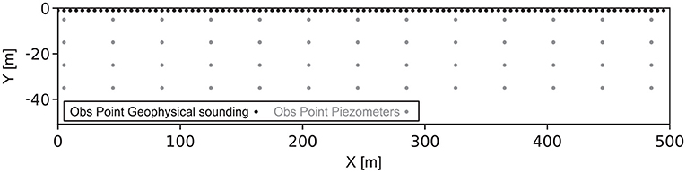
Figure 5. Location of the geophysical and hydrogeological observation points. The river is located at the position (500,0).
The second physical forward is a transient groundwater model based on the MODFLOW 6 code (Langevin et al., 2017; Hughes et al., 2017) interfaced with the FloPy package (Bakker et al., 2016). We consider the propagation and attenuation of a periodic perturbation on the upper right corner of the model (Figure 4). The river level at his location changes daily following a sinusoidal curve. This can mimic either tidal or daily discharge variations. The river is assumed to be connected to the aquifer with a conductance of 10−2 [m2s−1]. A second signal comes from a uniform recharge varying in time at the top of the model. We assume a no-flow boundary on the other sides of the model. Heads are recorded at 52 observation points in the model (Figure 5). The simulation lasts for 10 days, with a time step of 15 min. However, since most of the signal comes from the upper right corner, we expect a decreasing contribution of the observations to the inversion toward the left. Since the aquifer is supposed to be heterogeneous and of fluvial origin, we consider that the geological heterogeneity below the river bed can be modeled using the same parameters as the aquifer. Our synthetic model does not consider the river bed as a special compartment and does include any transient effect on the conductance of the river bed.
The computing time needed for the two forward models is drastically different. Geophysical forward takes about 2 s per model, when the transient hydraulic forward needs 30 s. The data used for the inversion are generated on a synthetic reference model and disturbed with Gaussian noise.
To better understand how the proposed methodology performs, we first present the results of the intermediate step (low-fidelity step) before providing detailed results after the final high-fidelity step.
For case C1, the number of ES-MDA iterations was set to 2 for the low fidelity step. The computing time was about 3 min on a personal computer. The mean residual decreased by 48% after one iteration and 62% after two iterations with respect to the unconditioned prior. Figure 6A shows the prior distribution for the position of the bottom of the aquifer for Model C1: it follows a normal distribution with an average depth of 38 m and 95% (2σ) of the simulated surfaces are between −26.8 and −49.2 m depth. This figure also shows the results of the inversion step: the average surface (solid black line) over the 100 members of the ensemble, the 95% confidence interval (gray shaded area), and the reference (in red). We see that even with a relatively small number of iterations and a small ensemble size, the ES-MDA algorithm converges rapidly to a plausible solution, even with the high simplification of the model. The reference surface is almost always within the predicted uncertainty range.
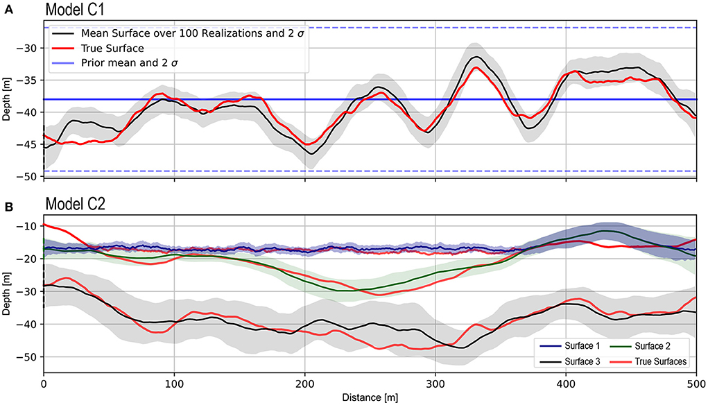
Figure 6. Low-fidelity inversion results for models C1 (A) and C2 (B) over 100 members and two iterations each. The model C1 has only one surface, and the model C2 has three surfaces. The shading areas correspond to 2 σ.
For case C2, Figure 6B shows the three average surfaces of 100 members. The computing time was about 3.5 min on a personal computer. In general, the inversion manages to correctly predict the depth of the transition and has identified the presence of the clay layer in the middle of the aquifer. If we compare surface 3 with its equivalent in the C1 model, we can denote that the corresponding uncertainty associated is much larger, even if the surfaces are exactly similar in terms of parameters and prior. This behavior is probably due to the presence of additional layers which imply some variations in the average resistivity above this surface that are much larger than in Case 1. Another interesting thing to denote are the fact that the surfaces 1 and 2 in the last 100 m of the model are superimposed. Where the lower surface equals the upper one, this last then follows the lower surface and becomes one with it. This is a complex hierarchical principle, because a whole set of parameters suddenly have no effect on the model residual. ES-MDA as correctly identified this logic from the set of prior models. It illustrates that using ES-MDA with geological priors could help reaching complexity in the inversion not seen so far.
For cases C1 and C2, 15 iterations were performed. The total run time was about 8 hours on a personal computer, mainly due to solving the transient hydrogeological forward problem. Figure 7A shows the average electrical resistivity and hydraulic conductivity (Figure 7D) over the ensemble of models at the end of the high-fidelity step. The corresponding uncertainties are shown in Figures 7B,E, while the reference model is shown in Figures 7C,F. No weighting based on the residual is used for the calculation of the mean model. The lower clay layer shows little uncertainty for both parameters. This is probably due to its very low resistivity and hydraulic conductivity within the range of possible values, which makes them easily identifiable. Another factor is probably that this layer was already well resolved during the low-fidelity step, because of its monofacies characteristic. However, we denote an important uncertainty on the exact depth of the transition on both parameter fields. It is only slightly updated compared to the uncertainty estimated after the low-fidelity step.
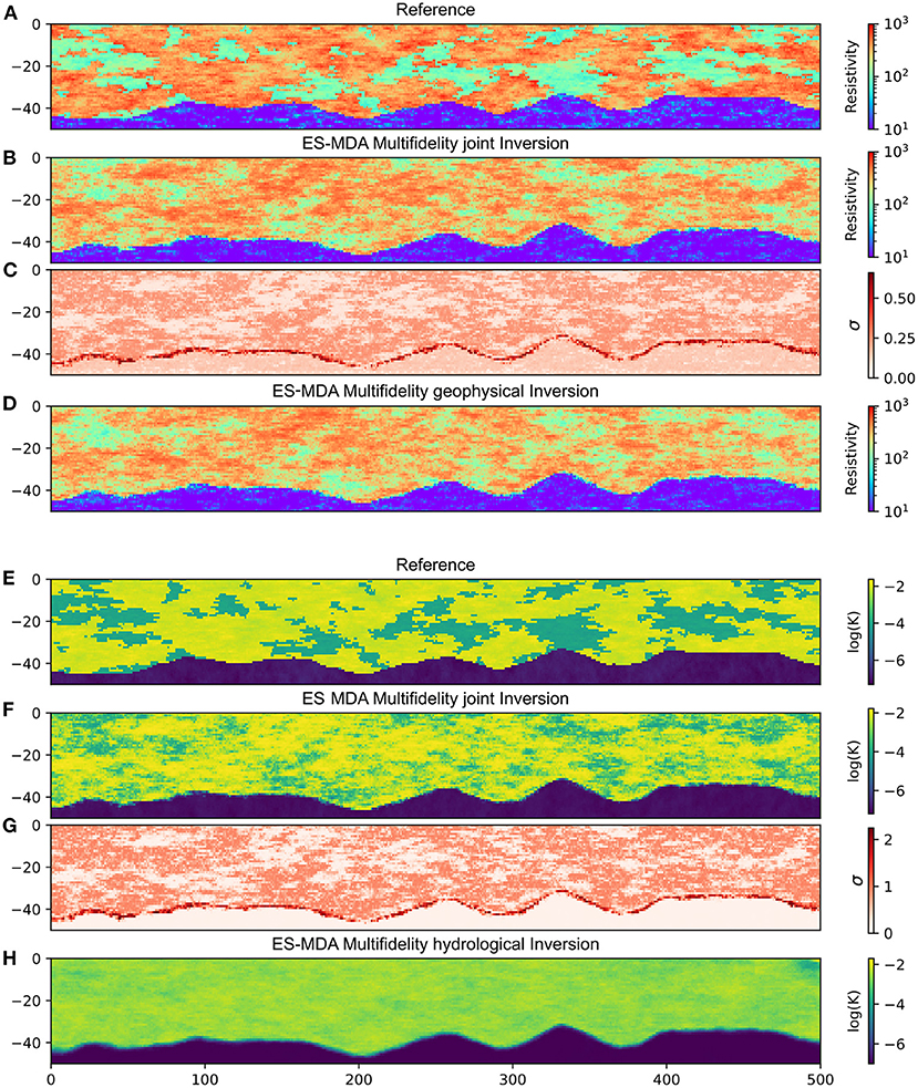
Figure 7. High-fidelity results for case C1. (A) Reference resistivity field, (B) mean model of resistivity, (C) resistivity uncertainty, (D) mean model for an application of the ES-MDA algorithm only using resistivity data, (E) permeability reference, (F) mean model of permeability, (G) permeability uncertainty, and (H) is the mean model for an application of the ES-MDA algorithm only using hydrological data.
The aquifer layer presents much higher variability for both parameters. First, we can denote that both fields seem spatially correlated. ES-MDA has correctly identified the correlation infused by the facies affiliation of the parameter field. More resistive zones are associated with more permeable areas, whereas less resistive zones are associated with less permeable sand. The uncertainty on the hydraulic conductivities is higher than the one associated with the resistivity, probably because the geophysical method is an active one, whereas our hydrological scenario is passive and extremely diffuse. Consequently, it is a more difficult problem to solve for the algorithm. This can also be denoted in Figures 7G,H.
Two High-Fidelity ES-MDA inversions were performed using one single dataset at a time. Not using the joint inversion approach has only a limited effect on the resistivity, compared to the joint inversion, even if some of the simulations can be marginally less noisy. On the other hand, inverting the hydraulic conductivities only shows a clear decrease in terms of the quality of the inversion. The mean simulation tends to converge to a hydraulic conductivities value intermediate between the sand and the gravel facies values. As mentioned above, this is expected because of the aquifer's high heterogeneity and the method's diffuse aspect. The only area clearly resolved is the upper right corner where the oscillating river limit is set. Since these cells control how the signal gets into the aquifer, they have a strong influence on all the observation points and are consequently easier to resolve for the ES-MDA algorithm.
Case C2 is more complex because the middle clay layer creates additional spatial variability and discontinuities. However, the same number of iterations as for case C1 were performed. Figure 8A shows the result of the geophysical data inversion only using a classical inversion based on a deterministic Newton-Gauss minimization using AarhusInv (Auken et al., 2015). Due to the diffusive nature of the geophysical method, the resulting model is significantly smoother than the reference (Figure 8C). The result of the ES-MDA inversion shows much sharper boundaries (Figure 8B) thanks to the embedding of the geological prior in the inversion method and the multi-fidelity approach.
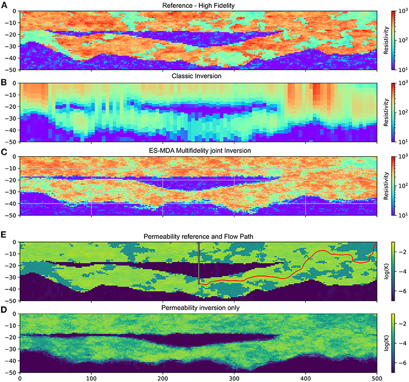
Figure 8. High-fidelity results for model C2. (A) Reference field for resistivity. (B) Resistivity field from a deterministic inversion. (C) ES-MDA inverted resistivity field. (D) Reference field for hydraulic conductivities with are well and the simulated steady-state flow line. (E) Mean model for an application of the ES-MDA algorithm on hydraulic conductivities only.
Figure 8D shows the results of the ES-MDA inversion on the hydraulic conductivities only. Unlike model C1, this result shows a better identification of numerous discontinuities in the field of hydraulic conductivities. We interpret this difference as follows: the contrast of hydraulic conductivities being sharper in case C2, more information can be captured by the hydrogeological data. This result confirms that the poor identification of the spatial distribution of the hydraulic conductivities for case C1 was simply the result of a lack of information in the hydrogeological data set.
Another interesting result is the comparison between the classic ES-MDA “monofidelity” approach and the multifidelity approach. In a classic ES-MDA approach, data assimilation is done directly on the whole parameter fields, with no LF step. In other words, the classic ES-MDA inversion is only the HF, with the difference that the starting models are drawn in the full space of the prior and not in the reduced space constrained by the ensemble of LF models. Figures 9A–C and Figures 9D–F compare the results of the classic ES-MDA inversion and the multifidelity one. For both parameters, we can first denote that the simulations are visually more noisy than multifidelity simulations. The boundaries between the bodies are better defined in multifidelity. The continuity of the geological structures is also better established. The same number of iterations was performed on both. Figure 9G shows the mean residuals in relation to the computation time. The two iterations of the LF took only about 3.5 min. We can see a slight increase in the residual between the last LF iteration and the first HF iteration. But the absolute value is much lower than the monofidelity one. In terms of computing time, it is interesting to note that even if the absolute number of forward calls and of ES-MDA loops is the same, the multifidelity is faster. The geophysical forward is almost not affected by the complexity of the model to simulate. However, the direct transient hydrological problem can show significant computing time variations depending on the hydraulic conductivity field. The first iterations are significantly slower, due to more complex models with high and abrupt hydraulic conductivity contrasts, for example. These results show that the use of the multifidelity approach tends to produce more realistic models, geologically speaking, with a shorter or equivalent computing time.
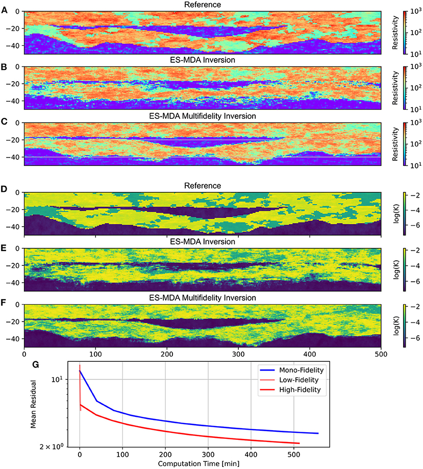
Figure 9. (A–F) Comparison between the inversion model resulting from a classic ES-MDA inversion, the multifidelity ES-MDA inversion, and the reference model for both the hydraulic conductivities and resistivity fields. (G) The residuals vs. the computation time for the classical ESMDA (monofidelity) and the multifidelity model.
To further test the predictive capacity of the approach, we consider an additional hydrogeological scenario. We implement a well at position x = 250 m reaching a depth z = −35 m. The well is only screened along the last meter. Taking into account an hourly pumping rate of 36 m3/h, we calculated the path and travel time needed for the pollution introduced in the river to reach the well of water production. Such scenarios and questions are common for various applications in hydrogeology. Figure 8E shows the reference path, going from the upper right corner river to the well in 37.5 days (advective time). The same computation was conducted for all prior and posterior models, as well as for all models obtained using the classical ESMDA joint inversion. The results of the flow path computations are shown in Figures 10A,B,D. The reduction of the uncertainty on the envelope of the possible flow paths is clear between the prior distribution and the results of the two inversions. The two inversions provide similar results, with a proper estimation of the flow path compared to the reference. The classic ESMDA inversion tends to show a narrower uncertainty. The distribution of the transit times of a pollutant between the river and the well are displayed on Figure 10C. The ES-MDA multi-fidelity ensemble predicts an arrival time of the pollutant between 35.75 and 87.1 days (10–90%interval) after injection. The prior gives a range between 21.5 and 10,000 days (10–68% interval) with 32% of the models predicting that the pollutant will not reach the well. The classical (mono-fidelity) ESMDA inversion ensemble predicts an arrival of the pollutant between 30.50 and 48.01 days (10–90%interval). Again, both inversions perform well, with a narrower time range for the classical ES-MDA inversion.
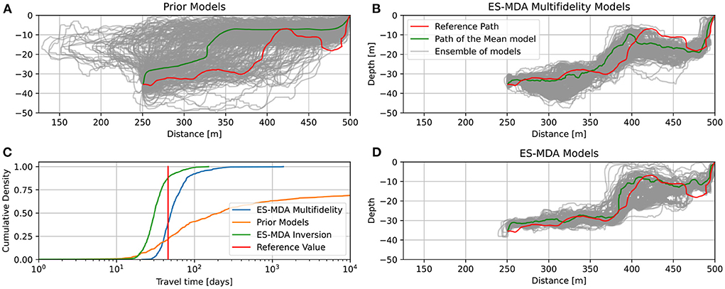
Figure 10. (A,B) Flow lines for the prior and posterior multifidelity ensemble of model C2. (C,D) Distribution of the travel time from the river to the well and Flow lines for the posterior monofidelity ensemble of model C2.
The proposed multi-fidelity ES-MDA inversion has successfully identified sharp and complicated geological models.
When a Bayesian MCMC algorithm may take one or a few weeks to converge and generate an ensemble of realizations matching the data, the proposed approach only needs a few hours. Although several limitations still exist. First of all, our reference model was generated using the same covariance models as the prior. As shown by Juda et al. (2022), the choice of an erroneous geostatistical prior can drastically decrease the realism and convergence rate of the inversion algorithm. This choice was straightforward in our synthetic approach but could be trickier when applying the method to real data sets. The solution requires properly analyzing all available field data to identify the required geostatistical parameters. If data are not sufficient to constrain the prior model, a possible solution would be to use published data from analog sites and generate a broad ensemble of models using different priors. The issue would then be to have a sufficient number of members to cover the whole prior parameter space and ensure that the ES-MDA algorithm would not create models that would be too far from reasonable geological models.
Another limitation of the inversion or data assimilation process is that we considered the noise in the data to be uncorrelated. This assumption is commonly used to treat each residual data point independently. In the synthetic case, this assumption is valid but could become problematic on real and strongly correlated data noise. Finally, the ES-MDA inversion (both in high- and low-fidelity) is not bounded to generate models that remain within the prior. It can be an advantage in the case of an uncertain prior, but it can also become a challenge if the algorithm generates physically impossible parameters.
The groundwater model used for the synthetic case C1 is not very informative as illustrated by the poor results obtained with hydrogeological data alone (Figure 7). Indeed, since the river is the only varying boundary condition applied to the model, only hydraulic conductivities close to the river are inferred with reduced uncertainty. This suggests that a large ensemble of hydraulic conductivity distributions is compatible with the data and that it is difficult for ES-MDA to approach the reference. Increasing the size of the ensemble could extend the possibilities and improve the results. However, the computational cost would also increase significantly. It is likely that using different hydrogeological situations, such as including pumping tests or tracer tests, would improve the identifiability of the hydraulic conductivity. Nevertheless, our results strengthen the advantage of using a joint inversion: the geophysical data help infer most of the subsurface structures and the spatial distribution of hydraulic conductivities. This contribution of geophysics is due to the fact that the different physical parameters are spatially correlated via the underlying litho-facies.
The main contribution of this paper is to propose to split the ES-MDA algorithm in two steps using a multi-fidelity strategy. We show that starting with the LFMs accelerates the inversion procedure significantly. It allows one to quickly delineate the main structures of the subsurface and quantify uncertainty. However, as it relies on a simplified version of the model, it cannot reproduce the reference in some places (Figure 6). This is a consequence of using homogeneous units (in terms of properties); thus, it is not possible to account for some important local variations of facies, and these have a significant impact on the geophysical data. Using different homogeneous values among the different members (or models) of the initial ensemble mitigates this effect by enlarging the uncertainty and allows one to identify the depth of the true surface accurately almost everywhere (Figure 6). However, it is clear that the uncertainty that we propagate in the second step of the inversion has a significant impact on the results. For example, if we consider the high value of the surface at around 330 m for case C1 (Figure 6A). The true surface is barely contained within the range of uncertainty, it means that the majority of the models considered the surfaces higher than the reference. As a consequence in the second step, ES-MDA compensates by predicting mostly “gravel” (high resistivity/permeability) just above this location, where normally there should be a relatively large area of “sand” (low resistivity/permeability, Figure 7). We then understand that small initial errors can have major impacts and that we should be careful with the final models. However, it should also be mentioned that the generated geological models are totally unconstrained. It is certain that incorporating more geological knowledge (such as borehole data) into the models would have helped to detect and solve this kind of inconsistency.
Our hydrogeological scenario involves 13 multilevel piezometers uniformly distributed over 500 m length. Even if some field sites show similar or even higher density of data, in a real application the density of piezometric information could be lower. The consequence will be a higher uncertainty associated with the permeability field. A preliminary sensitivity analysis on our synthetic models showed that removing two piezometers either close to the source of the signal or far from it have drastically different effects on the final uncertainty. This is simply due to the difference in the amount of information carried by the two data series. In addition, in our synthetic example, we considered rather simple boundary conditions (such as a sinusoidal variation of the river level) without any uncertainty. In practice, it would be straightforward to cope with more complex boundary conditions, such as time-varying water levels. For the uncertainty on the boundary conditions, the proposed approach would be to include these boundary conditions as parameters within the ESMDA inversion, this would result in a higher level of uncertainty for the overall aquifer characterization.
Finally, we think that the approach proposed in this paper could be applied to a wide range of problems. We illustrate here the multi-fidelity idea using a simpler geological model and a faster forward operator at the same time. However, many other combinations could be tested: for example, the low-fidelity model could correspond to a steady-state hydrogeological model and the high-fidelity model could be the full transient model. Another possibility could be to use only a few geophysical observation points for the low-fidelity step and a complete detailed data set for the high-fidelity step. One could also group geological units to simplify the geological architecture during the low-fidelity step.
The results presented in this paper demonstrate that ES-MDA, multi-fidelity, and ArchPy, all together, can constitute a potentially powerful framework for performing geologically consistent inversions. The proposed approach allows integrating in a consistent and stochastic manner different types of data and thus reducing the global uncertainty on groundwater models. The use of the multi-fidelity approach on such a problem has proven to be more efficient in infusing prior geological knowledge into the inversion. This has resulted in more realistic geological models while being faster. Future work includes the application of the presented methodology to real 3D field data.
Several main conclusions can be drawn from this research:
• ES-MDA is an efficient tool to get an ensemble of plausible hydrogeological models in a multi-fidelity framework.
• Hierarchical multi-fidelity helps to keep models geologically consistent during the inversion process while improving the quality of the models.
• Hydrogeophyiscal joint inversions can be decomposed and improved within a multifidelity and hierarchical framework.
• ArchPy's models are useful priors to investigate subsurface uncertainty.
The original contributions presented in the study are included in the article/supplementary material, further inquiries can be directed to the corresponding author.
AN, LS, and PR contributed to the design of the study and wrote and revised the original draft. AN and LS implemented and developed the inversions. PR obtained funding and supervised the work. All authors contributed to the article and approved the submitted version.
This research was supported by the Swiss National Science Foundation through the project Phenix (grant no. 182600).
The authors would like to thank Julien Straubhaar for his support for the implementation of a part of the geostatistical algorithms, and for heling us identifying bugs in the code. Finally, we warmly thank Erwan Gloaguen for his ideas concerning the use of ES-MDA.
The authors declare that the research was conducted in the absence of any commercial or financial relationships that could be construed as a potential conflict of interest.
All claims expressed in this article are solely those of the authors and do not necessarily represent those of their affiliated organizations, or those of the publisher, the editors and the reviewers. Any product that may be evaluated in this article, or claim that may be made by its manufacturer, is not guaranteed or endorsed by the publisher.
Anderson, J. L. (2001). An ensemble adjustment Kalman filter for data assimilation. Month. Weath. Rev. 129, 2884–2903. doi: 10.1175/1520-0493(2001)129<2884:AEAKFF>2.0.CO;2
Asher, M. J., Croke, B. F., Jakeman, A. J., and Peeters, L. J. (2015). A review of surrogate models and their application to groundwater modeling. Water Resour. Res. 51, 5957–5973. doi: 10.1002/2015WR016967
Auken, E., Christiansen, A. V., Kirkegaard, C., Fiandaca, G., Schamper, C., Behroozmand, A. A., et al. (2015). An overview of a highly versatile forward and stable inverse algorithm for airborne, ground-based and borehole electromagnetic and electric data. Explor. Geophys. 46, 223–235. doi: 10.1071/EG13097
Auken, E., Foged, N., Larsen, J. J., Lassen, K. V. T., Maurya, P. K., Dath, S. M., et al. (2019). tTEM?a towed transient electromagnetic system for detailed 3d imaging of the top 70 m of the subsurface. Geophysics 84, E13?-E22. doi: 10.1190/geo2018-0355.1
Bakker, M., Post, V., Langevin, C. D., Hughes, J. D., White, J. T., Starn, J., et al. (2016). Scripting modflow model development using python and flopy. Groundwater 54, 733–739. doi: 10.1111/gwat.12413
Barfod, A. A. S., Møller, I., Christiansen, A. V., Høyer, A.-S., Hoffimann, J., Straubhaar, J., et al. (2018). Hydrostratigraphic modeling using multiple-point statistics and airborne transient electromagnetic methods. Hydrol. Earth Syst. Sci. 22, 3351–3373. doi: 10.5194/hess-22-3351-2018
Carle, S. F., and Fogg, G. E. (2020). Integration of soft data into geostatistical simulation of categorical variables. Front. Earth Sci. 8:565707. doi: 10.3389/feart.2020.565707
Chen, Y., and Oliver, D. S. (2011). Ensemble randomized maximum likelihood method as an iterative ensemble smoother. Math. Geosci. 44, 1–26. doi: 10.1007/s11004-011-9376-z
Christensen, N. K., Minsley, B. J., and Christensen, S. (2017). Generation of 3-D hydrostratigraphic zones from dense airborne electromagnetic data to assess groundwater model prediction error. Water Resour. Res. 53, 1019–1038. doi: 10.1002/2016WR019141
Dagasan, Y., Juda, P., and Renard, P. (2020). Using generative adversarial networks as a fast forward operator for hydrogeological inverse problems. Groundwater 58, 938–950. doi: 10.1111/gwat.13005
Deutsch, C. V. (2002). Geostatistical Reservoir Modeling. Applied Geostatistics Series. Oxford; New York, NY: Oxford University Press.
Deutsch, C. V., and Journel, A. G. (1992). GSLIB. Geostatistical Software Library and User?s Guide. New York, NY: Oxford University Press.
Emerick, A. A. (2016). Analysis of the performance of ensemble-based assimilation of production and seismic data. J. Petrol. Sci. Eng. 139, 219–239. doi: 10.1016/j.petrol.2016.01.029
Emerick, A. A., and Reynolds, A. C. (2013). Ensemble smoother with multiple data assimilation. Comput. Geosci. 55, 3–15. doi: 10.1016/j.cageo.2012.03.011
Gaspari, G., and Cohn, S. E. (1999). Construction of correlation functions in two and three dimensions. Q. J. R. Meteorol. Soc. 125, 723–757. doi: 10.1002/qj.49712555417
Graf, H. R., and Burkhalter, R. (2016). Quaternary deposits: concept for a stratigraphic classification and nomenclature?an example from northern Switzerland. Swiss J. Geosci. 109, 137–147. doi: 10.1007/s00015-016-0222-7
Høyer, A.-S., Jørgensen, F., Sandersen, P., Viezzoli, A., and Møller, I. (2015). 3D geological modelling of a complex buried-valley network delineated from borehole and AEM data. J. Appl. Geophys. 122, 94–102. doi: 10.1016/j.jappgeo.2015.09.004
Hughes, J. D., Langevin, C. D., and Banta, E. R. (2017). “Documentation for the MODFLOW 6 framework,” in Techniques and Methods. US Geological Survey. doi: 10.3133/tm6A57
Irving, J., and Singha, K. (2010). Stochastic inversion of tracer test and electrical geophysical data to estimate hydraulic conductivities. Water Resour. Res. 46. doi: 10.1029/2009WR008340
Jardani, A., Revil, A., and Dupont, J. (2013). Stochastic joint inversion of hydrogeophysical data for salt tracer test monitoring and hydraulic conductivity imaging. Adv. Water Resour. 52, 62–77. doi: 10.1016/j.advwatres.2012.08.005
Jørgensen, F., Høyer, A.-S., Sandersen, P. B., He, X., and Foged, N. (2015). Combining 3D geological modelling techniques to address variations in geology, data type and density?An example from Southern Denmark. Comput. Geosci. 81, 53–63. doi: 10.1016/j.cageo.2015.04.010
Journel, A. G. (1983). Nonparametric estimation of spatial distributions. J. Int. Assoc. Math. Geol. 15, 445–468. doi: 10.1007/BF01031292
Journel, A. G., and Isaaks, E. H. (1984). Conditional indicator simulation: application to a Saskatchewan uranium deposit. J. Int. Assoc. Math. Geol. 16, 685–718. doi: 10.1007/BF01033030
Juda, P., Straubhaar, J., and Renard, P. (2022). Comparison of three recent discrete stochastic inversion methods and influence of the prior choice. Compt. Rendus. Géosci. 355. doi: 10.5802/crgeos.160
Kalman, R. E. (1960). A new approach to linear filtering and prediction problems. Trans. ASME J. Basic Eng. Ser. D 82, 35–45. doi: 10.1115/1.3662552
Kang, X., Shi, X., Revil, A., Cao, Z., Li, L., Lan, T., and Wu, J. (2019). Coupled hydrogeophysical inversion to identify non-Gaussian hydraulic conductivity field by jointly assimilating geochemical and time-lapse geophysical data. J. Hydrol. 578:124092. doi: 10.1016/j.jhydrol.2019.124092
Lam, D.-T., Kerrou, J., Renard, P., Benabderrahmane, H., and Perrochet, P. (2020). Conditioning multi-gaussian groundwater flow parameters to transient hydraulic head and flowrate data with iterative ensemble smoothers: a synthetic case study. Front. Earth Sci. 8:202. doi: 10.3389/feart.2020.00202
Langevin, C. D., Hughes, J. D., Banta, E. R., Niswonger, R. G., Panday, S., and Provost, A. M. (2017). Documentation for the Modflow 6 Groundwater Flow Model. Technical Report, US Geological Survey. doi: 10.3133/tm6A55
Linde, N., and Doetsch, J. (2016). “Joint inversion in hydrogeophysics and near-surface geophysics,” in Integrated Imaging of the Earth, eds Moorkamp, M., Lelièvre, P. G., Linde, N., and Khan, A (Hoboken, NJ: John Wiley & Sons, Inc.), 117–135. doi: 10.1002/9781118929063.ch7
Mariethoz, G., Renard, P., and Straubhaar, J. (2010). The Direct Sampling method to perform multiple-point geostatistical simulations. Water Resour. Res. 46. doi: 10.1029/2008WR007621
Neven, A., Maurya, P. K., Christiansen, A. V., and Renard, P. (2021). tTEM20aar: a benchmark geophysical data set for unconsolidated fluvioglacial sediments. Earth Syst. Sci. Data 13, 2743–2752. doi: 10.5194/essd-13-2743-2021
Schorpp, L., Straubhaar, J., and Renard, P. (2022). Automated hierarchical 3d modeling of quaternary aquifers: the ArchPy approach. Front. Earth Sci. 10:884075. doi: 10.3389/feart.2022.884075
van Leeuwen, P. J., and Evensen, G. (1996). Data assimilation and inverse methods in terms of a probabilistic formulation. Month. Weath. Rev. 124, 2898–2913. doi: 10.1175/1520-0493(1996)124<2898:DAAIMI>2.0.CO;2
Wang, L., Kitanidis, P. K., and Caers, J. (2022). Hierarchical bayesian inversion of global variables and large-scale spatial fields. Water Resour. Res. 58. doi: 10.1029/2021WR031610
Wen, X.-H., and Chen, W. (2005). “Real-time reservoir model updating using ensemble Kalman filter,” in SPE Reservoir Simulation Symposium SPE 92991 (The Woodlands, TX). doi: 10.2118/92991-MS
White, J. T. (2018). A model-independent iterative ensemble smoother for efficient history-matching and uncertainty quantification in very high dimensions. Environ. Model. Softw. 109, 191–201. doi: 10.1016/j.envsoft.2018.06.009
Xu, T., Zhang, W., Gómez-Hernández, J. J., Xie, Y., Yang, J., Chen, Z., and Lu, C. (2022). Non-point contaminant source identification in an aquifer using the ensemble smoother with multiple data assimilation. J. Hydrol. 606:127405. doi: 10.1016/j.jhydrol.2021.127405
Zheng, Q., Zhang, J., Xu, W., Wu, L., and Zeng, L. (2019). Adaptive multifidelity data assimilation for nonlinear subsurface flow problems. Water Resour. Res. 55, 203–217. doi: 10.1029/2018WR023615
Keywords: multi-fidelity, joint inversion, stochastic, hierarchical modeling, multiple data assimilation, Ensemble Smoother (ES)
Citation: Neven A, Schorpp L and Renard P (2022) Stochastic multi-fidelity joint hydrogeophysical inversion of consistent geological models. Front. Water 4:989440. doi: 10.3389/frwa.2022.989440
Received: 08 July 2022; Accepted: 04 October 2022;
Published: 20 October 2022.
Edited by:
Thomas Graf, Leibniz University Hannover, GermanyReviewed by:
Luk J. M. Peeters, CSIRO Land and Water, AustraliaCopyright © 2022 Neven, Schorpp and Renard. This is an open-access article distributed under the terms of the Creative Commons Attribution License (CC BY). The use, distribution or reproduction in other forums is permitted, provided the original author(s) and the copyright owner(s) are credited and that the original publication in this journal is cited, in accordance with accepted academic practice. No use, distribution or reproduction is permitted which does not comply with these terms.
*Correspondence: Alexis Neven, YWxleGlzLm5ldmVuQHVuaW5lLmNo
Disclaimer: All claims expressed in this article are solely those of the authors and do not necessarily represent those of their affiliated organizations, or those of the publisher, the editors and the reviewers. Any product that may be evaluated in this article or claim that may be made by its manufacturer is not guaranteed or endorsed by the publisher.
Research integrity at Frontiers
Learn more about the work of our research integrity team to safeguard the quality of each article we publish.