 Sneha Santy
 Pradeep Mujumdar
 Govindasamy Bala
- 1Interdisciplinary Centre for Water Research, Indian Institute of Science, Bangalore, India
- 2Department of Civil Engineering, Indian Institute of Science, Bangalore, India
- 3Centre for Atmospheric and Oceanic Sciences, Indian Institute of Science, Bangalore, India
The industrialized stretch of Kanpur is considered to be one of the most polluted stretches of the Ganga River, with untreated sewage, industrial discharge, and agricultural runoff. Risk assessment studies on water quality for future scenarios are limited for this stretch of the river. In this study, we assess the effect of climate change on water quality, the risk of eutrophication, and fish kill for the mid and end of the twenty-first century for this river stretch. The water quality parameters considered are dissolved oxygen (DO), biochemical oxygen demand (BOD), ammonia, nitrate, total nitrogen (TN), organic-, inorganic- and total phosphorous (TP), and fecal coliform (FC). The risk of eutrophication and fish kill are quantified using simulated concentrations of nutrients and DO, respectively. Downscaled climate change projections for two climate change scenarios (RCP4.5 and RCP8.5) are used to drive a hydrological model coupled to a water quality simulation model. Our simulations indicate a potential deterioration of water quality in this stretch in the mid-twenty-first century, with a potential increase in pollutant concentration by more than 50% due to climate change alone. However, a slight improvement is simulated by the end of the century relative to the mid-twenty-first century which can be attributed to increased streamflow during low-flow periods due to increased summer mean precipitation. The risk of reduced dissolved oxygen and increased organic and nutrient pollution, and the risk of eutrophication and fish kill increase with warming due to the rise in the frequency of low-flow events and a reduction in streamflow during low-flow events. However, the risk of nitrate and microbial pollution is reduced because of an increased denitrification rate and pathogen decay rate with warming. The risk of eutrophication and fish kill is found to increase by 43.5 and 15% due to climate change alone by mid-twenty-first century. Our findings could be helpful to planners in water resource management to take necessary actions to improve the water quality of the Ganga River in this century.
Introduction
The Ganga River pollution is a significant environmental issue in India. Due to its high religious importance, a clean Ganga River is a dream for many Indians. Large quantities of untreated sewage, industrial discharge, and agricultural runoff have led to deterioration of the Ganga water quality [(Consortium of 7 “Indian Institute of Technology” s (IITs), 2013)]. The Ganga Action Plan (GAP) was initiated in 1986 to improve the Ganga water quality to Bathing standards (National River Conservation Directorate Ministry of Environment Forests, 2009): however, this goal has not been reached for the entire river stretch so far. As per the Central Pollution Control Board (CPCB) statistics of 2011, more than 60% of industrial pollutants are from the industrial city of Kanpur, and hence Kanpur is identified as the pollution hotspot of the river (Central Pollution Control Board, 2013). The ongoing climate change can aggravate the water pollution, especially when the pollutant loadings to the river, such as industrial discharge, municipal sewage, and agricultural runoff are large. Therefore, it is essential to study the impact of climate change on Ganga water quality and its associated risk in this highly industrialized stretch for developing or modifying any policy for a cleaner Ganga in the future.
Climate change could affect water quality by changing the stream temperature and streamflow, mainly driven by air temperature and precipitation (Rehana and Mujumdar, 2011). Previous studies (Carmichael et al., 1996; Caruso, 2002; Ducharne et al., 2006; Cox and Whitehead, 2009; Bharati et al., 2011; Ficklin et al., 2013; Whitehead et al., 2015b; Javadinejad et al., 2021) show that an increase in stream temperature and reduced streamflow during the dry season under climate change could lead to reduced water quality in terms of dissolved oxygen, electrical conductivity, sediment concentration. The water quality projections are also affected by land use land cover change, mainly the expansion of agricultural land, which can lead to an increased nutrient concentration (Gyawali et al., 2013; Ostad-Ali-Askari et al., 2017; Permatasari et al., 2017; Davids et al., 2018; Jacobs et al., 2018; Namugizea et al., 2018; Santy et al., 2020; Shayannejad et al., 2022). Population growth and industrial activities could lead to increased water demand and sewage (Khattiyavong and Lee, 2019; Ostad-Ali-Askari, 2022) and consequently deterioration in water quality (Khan et al., 2017).
Some past studies have identified climate change as a more influential factor than land use or socio-economic factors for the Ganga river water balance (Jain and Singh, 2018; Saha and Ghosh, 2020), and hence it is valuable to study the isolated effects of climate change on the Ganga water quality. A previous study on climate and land use land cover impact on Ganga River (Santy et al., 2020) using hypothetical scenarios and a stand-alone water quality model showed an increase in organic and nutrient pollution and a decrease in dissolved oxygen (DO) and microbial pollution due to warming and reduction in low flows. The increase in nutrient pollution and reduction in DO can lead to eutrophication and fish kill, respectively. In contrast, some studies on Ganga River have shown an increase in monsoon flows (Whitehead et al., 2015a) and improvement in water quality with respect to nitrogen and phosphorous concentrations for sustainable socio-economic scenario with climate change (Jin et al., 2015; Whitehead et al., 2015a,b).
Risk assessment in water quality studies is very limited and is typically quantified using statistical or stochastic methods such as multiple logistic regression, non-linear model, and fuzzy techniques (Mujumdar and Sasikumar, 2002; Rehana and Mujumdar, 2012; Liu et al., 2018). Recently, however, risk assessment of water supply under warming is analyzed using a coupled hydrological model and water quality model simulations, where turbidity and phosphorous concentration are considered (Mortazavi-Naeini et al., 2019). One of the critical effects of warming on surface water is eutrophication—the excess plant growth in fresh water due to enrichment of nutrients. The eutrophication is high in spring and summer seasons (plant growing season) due to more light levels and low flow, resulting in larger nutrient residence time, which accelerates algal growth (Nazari-Sharabian et al., 2018).
Several past studies have assessed the impact of climate change on nutrients (Bouraoui et al., 2002; Zweimuller et al., 2008; Dyer et al., 2014; Wang et al., 2018; Xu et al., 2020); however, these assessments have not quantified the effects of climate change on eutrophication and the associated risk. There are also several previous studies on eutrophication under warming (Peperzak, 2003; Edwards et al., 2006; Johnk et al., 2008; Kosten et al., 2011; Wells et al., 2015; Gittings et al., 2018), where the harmful algal blooms or phytoplankton are considered. However, these studies do not directly link nutrients to eutrophication and its associated risk under warming. In past studies, the risk of eutrophication is quantified using the chlorophyll a value (Walker, 1979; Carlson, 1991; Matthews et al., 2002; Adamovich et al., 2019), for which data is not readily available. In this study, we use an empirical equation to estimate chlorophyll a from nutrients and thus calculate the risk of eutrophication due to climate change.
Another risk associated with warming is fish kill, but studies on this are limited (Kibria, 2014). Freshwater fishes are more sensitive to an increase in water temperature than changes in flow characteristics (Barbarossa et al., 2021), and thus climate change can affect the growth, migration and even lead to the extinction of some fish species (Perry et al., 2005; Xenopoulos et al., 2005; Yan et al., 2011; Tedesco et al., 2013; Ding et al., 2016; Tao et al., 2018). Fish kill occurs due to reduced dissolved oxygen (DO) caused mainly by increased organic, nutrient, and microbial pollutant loads and eutrophication (Austin, 1998; Hansson and Brönmark, 2009; Dodds and Whiles, 2020). Several previous studies have assessed the change in DO with warming (Cox and Whitehead, 2009; Rehana and Mujumdar, 2011; Ficklin et al., 2013; Chapra et al., 2021); however, such studies have not linked DO with the fish kill. Predicting fish kill from dissolved oxygen can be an effective tool, as DO values of the river are readily available.
This study focuses only on isolating the effects of climate change on water quality and its associated risk and keeps the other factors such as point and non-point loads, land use, population, and industries unchanged for the future. The impact of other factors will be the subject of our future studies. The risk of reduced water quality, eutrophication, and fish kill is quantified using dynamic simulations with a coupled modeling framework. This framework can simulate the physical, chemical and biological processes with warming (Chapra and Pelletier, 2003), and hence is likely to provide reliable results. Further, the risk of eutrophication and fish kill is calculated from chlorophyll a and simulated DO values. The nine water quality parameters considered for the study are dissolved oxygen (DO), Biochemical oxygen demand (BOD), ammonia, nitrate, total nitrogen (TN), organic-, inorganic- and total phosphorous (TP), and fecal coliform (FC).
Thus, the main objectives of our study are (i) to assess the change in water quality for future climate change scenario and (ii) to quantify the risk of reduced water quality, eutrophication and fish kill using a comprehensive coupled hydrological and water quality modeling framework (Figure 1). The novelty of the work lies in the quantification of the individual contribution of climate change to the risk of reduced water quality, eutrophication and fish kill for a highly polluted stretch of Ganga River. The study area, data, models and methodology for the risk assessment are provided in Sections Study area and data and Methodology. Results are discussed in Section Results and discussion and conclusions are provided in Section Conclusion.
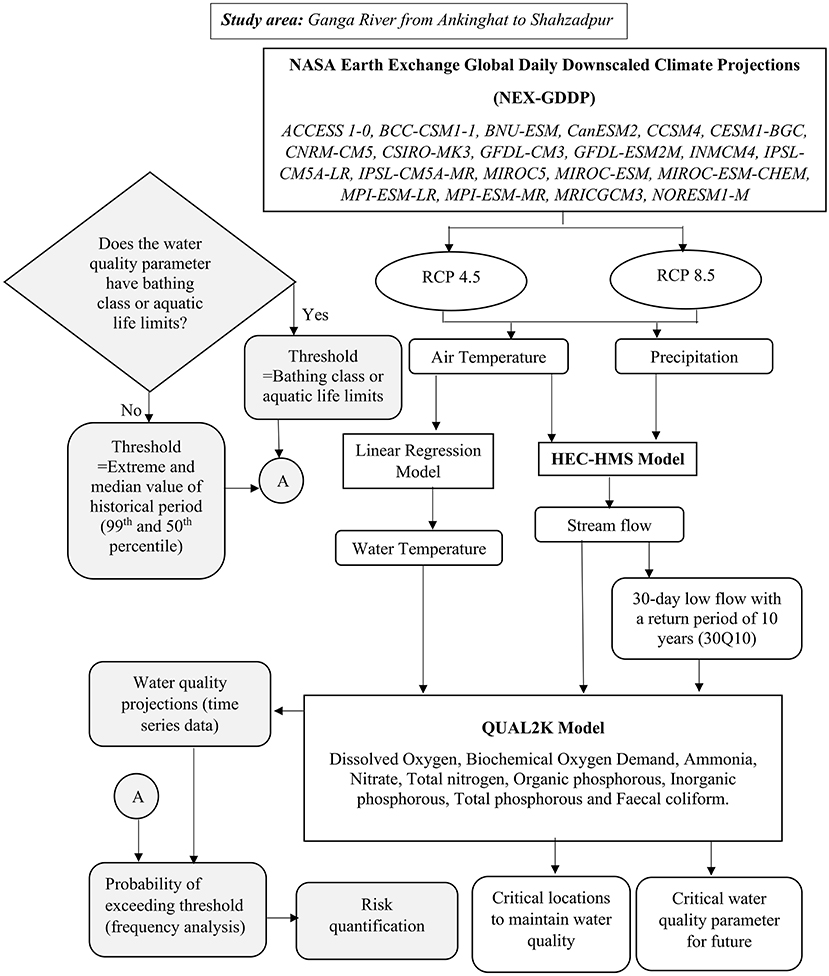
Figure 1. Overview of the work presented in this paper.
Study area and data
The Ganga River, the largest river basin in India, lies between 73°2'E to 89°5'E longitudes and 21°6'N to 31°21'N latitudes. The total length and the catchment area of the basin are 2,500 km and 8,61,404 sq. km, respectively. Ganga river has its origin in the great Himalayas. It flows through north India, Nepal, and Bangladesh, with 71% of the basin area in India covering the states Uttarakhand, Uttar Pradesh, Madhya Pradesh, Rajasthan, Haryana, Himachal Pradesh, Chhattisgarh, Jharkhand, Bihar, West Bengal, and Delhi, and finally empties into the Bay of Bengal. Ganga river basin has a varied topology with a wide range of elevation in the Upper Ganga basin up to Shahzadpur ranging from 29 to 7,796 m. The basin receives an average annual rainfall of 300–2,000 mm, with the bulk of rainfall occurring in the summer monsoon months. The low flow period is observed during the dry period of November to May (Whitehead et al., 2015b; Santy et al., 2020). The average temperature of the basin varies from a maximum of 30.3°C in the summer months to a minimum of 6.4°C in winter (Central Water Commission and National Remote Sensing Centre, 2014). Eutric Cambisols, which are suitable for cultivation, are the predominant soil type in the basin's lower part. Tannery, sugar and distillery, pulp and paper mills are the major industries discharging pollution to the Ganga River, with a high pollution load of BOD, Chemical oxygen demand (COD), solids, TN, chromium, sulfate, sulfide and chloride.
The highly industrialized stretch of Ganga River, 238 km from Ankinghat to Shahzadpur, passing through Kanpur, is considered as the study area for this paper. Figure 2 shows the study area with point loads and diffuse loads joining the river stretch, and Table 1 shows the details of the data used in the study and the data source. The drains from Kanpur, Jajmau, Unnao, and Pandu River join this stretch and its effluent characteristics is given in Supplementary Table S1. The Kanpur drains (KD) include Ranighat drain (KD1), Sisamau nala (KD2), Bhagwatdas nala (KD3), Golaghat nala (KD4), Satti chaura (KD5), Permiya drain (KD6), and Muir mill drain (KD7) with high ammonia and fecal coliform loading and low nitrate loading. Unnao drain (UD) consists of Loni drain (UD1) and City Jail drain (UD2), which carries high BOD and fecal coliform loading. Jajamu drains (JD) include Shetla bazar (JD1), Wazidpur drain (JD2) and Bhurighat drain (JD3), and carries high BOD, ammonia, nitrate, phosphorous and fecal coliform loading. Pandu river drains (PD) include Panki Thermal Power Plant drain (PD1), ICI drain (PD2), Ganda nalla (PD3), COD nalla (PD4), and Halwa Khanda nalla (PD5) carrying high BOD, ammonia and fecal coliform loading and moderate nitrate loading.
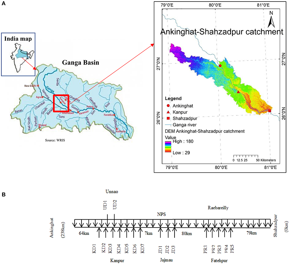
Figure 2. (A) Ganga basin with study area Ankinghat to Shahzadpur highlighted as a red box. Figure on right shows DEM of Ankinghat to Shahzadpur catchment with locations of Ankinghat, Kanpur and Shahzadpur marked; (B) Schematic diagram of pollutant loading in the study area, with drains from Kanpur (KD), Jajmau (JD), Unnao (UD) and Pandu river drains (PR), and non-point source pollution (NPS).
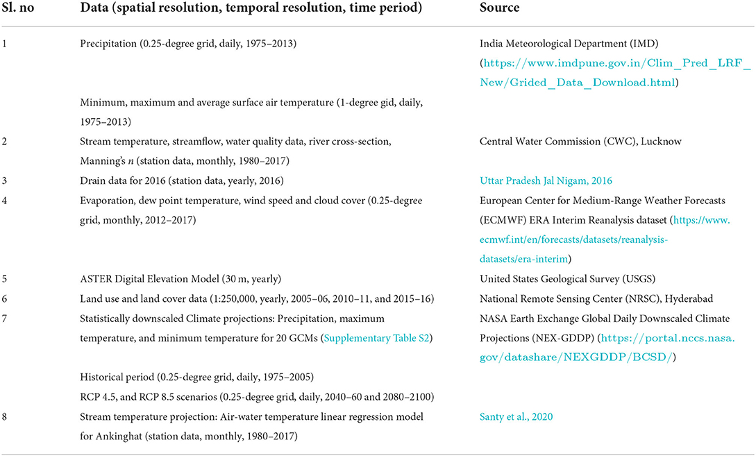
Table 1. Data used and its source.
Methodology
The hydrological model
The Hydrologic Engineering Center—Hydrologic Modeling System (HEC-HMS 4.3) (U. S. Army Corps of Engineers Hydrologic Engineering Center, 2000) (Supplementary Section S1), is used to simulate the streamflow at Ankinghat, the headwater for the water quality simulation. The HEC-HMS model has been found to perform well for streamflow simulation compared to other hydrological models (Sahu et al., 2020). Also, the HEC-HMS model is an open access software, and computational time required is less in comparison with other models. Hence, we have adopted the HEC-HMS model for the present study. Major components of the model are a basin model, meteorological models, control specification, and a time-series data manager (U. S. Army Corps of Engineers Hydrologic Engineering Center, 2000). The basin model is prepared using the HEC-GeoHMS module of ArcGIS, and the processed data is imported to the HEC-HMS model. This processing mainly consists of digital elevation model (DEM) processing, delineating streams and watershed characteristics, terrain processing, and basin processing.
The basin model has 45 subbasins. Seven temperature gauges and 139 precipitation gauges are created for the basin, and the time series data at a daily timescale is given as input to the model. The grid point data obtained from IMD is considered as gauge points. The precipitation for each subbasin is specified using the gauge weight method. The gauge points falling inside the sub-basin are given a weightage of 1, and the gauge points outside the sub-basin are given a weightage of 0.25. The meteorological model is created with Bristow-Campbell calculation for short wave radiation (Bristow and Campbell, 1984), gauge weight method for precipitation (Chow et al., 1988), and Priestley Taylor method for evapotranspiration (Chow et al., 1988). The default values of transmittance (0.7) and exponent (2.4) are used for the Bristow-Campbell Shortwave calculation. Each month's mean temperature range is also provided (U. S. Army Corps of Engineers Hydrologic Engineering Center, 2000). A dryness coefficient value of 1.3 is considered for the Priestley Taylor evapotranspiration method. Simple Canopy, Simple Surface, Deficit and Constant method, SCS Unit Hydrograph, Constant Monthly Baseflow, and Muskingum are the methods used for canopy, surface, loss, transform, baseflow, and routing, respectively.
The model is calibrated for the years 1977–2000 and validated for the years 2001–2012. An R2-value of 0.6 is obtained for both calibration and validation. The soil information is obtained from FAO, and the range of loss rates proposed by Skaggs and Khaleel (1982); SCS (1986), and U. S. Army Corps of Engineers Hydrologic Engineering Center (2000) is adopted (Supplementary Table S3). The maximum surface storage is obtained from the basin slope proposed by Bennett (1998) and Fleming (2002). The catchment has a very steep slope in the upstream portion due to the presence of the Himalayas, a gentle slope in the mid-stream, and flat, furrowed land downstream. Similarly, canopy interception is obtained from vegetation. The calibrated parameters are shown in Supplementary Table S4 and Supplementary Figure S1.
The calibration is performed with a normalized flow. The basin has major diversions such as Upper Ganga Canal, Middle Ganga Canal, East Ganga Canal, and Lower Ganga Canal, which abstract a significant amount of flow. As discharge data of these abstractions is the only data available, it is not modeled in HEC-HMS. Instead, the actual observed flow is added to the canal flows, which is the normalized flow, with which calibration is carried out.
Normalized flow = Actual flow at Ankinghat + flow at the diversions (Upper Ganga Canal, Middle Ganga canal, East Ganga Canal, and Lower Ganga Canal).
The calibration is performed with a combination of manual calibration and the model's optimization module. The parameters are optimized to minimize the root mean square error. The time series plot of streamflow calibration and validation is shown in Supplementary Figures S2a,b, and the flow duration curves for calibration and validation along with the flow statistics such as mean, median, standard deviation, MAM30, Q5, Q95, and R2 are shown in Supplementary Figures S2c,d. The results show good agreement for low flows (Q95 and MAM30); thus, the calibrated model is found to be suitable for climate change simulations.
The calibrated model is then used to simulate RCP 4.5 and RCP 8.5 climate change scenarios for 2040–60 and 2080–2100. The temperature and precipitation data are bias-corrected using the Quantile mapping method (Salvi et al., 2011). The daily bias-corrected precipitation, temperature, and monthly temperature corresponding to each climate change scenario are given as input to the model, keeping the model parameters canopy, surface, loss, transform, baseflow and routing kept unchanged. From the simulated daily streamflow values, the design low flow value of 30-day low flow with a return period of 10 years (30Q10) is calculated for each time slice and used as headwater streamflow input to the water quality simulation model, which is described next.
The water quality simulation model
QUAL2K is the water quality simulation model (Chapra and Pelletier, 2003) used for the study (Supplementary Section S2). QUAL2K is an open access software and has been used in many previous studies (Rehana and Mujumdar, 2012; Yang, 2013; Chaudhary et al., 2019). It can be driven by climatic inputs such as dew point temperature, wind speed, cloud cover and solar radiation to simulate water quality, and it is also a computationally efficient model. The inputs to the model are flow, stream temperature, water quality at the headwater, hydro geometric characteristics of the river reach such as width, depth, channel slope, side slope, manning's n, meteorological data such as air temperature, dew point temperature, wind speed, evaporation, cloud cover; point loads and diffuse loads. The point loads include industrial and domestic sewage discharge. Sewage is drained through major drains from Kanpur, Unnao, Jajmau, and Pandu River, and the flow and effluent characteristics of these drains are given as the point source input to the model. The non-point source is calculated using an export coefficient method (Santy et al., 2020) (Supplementary Section S3), wherein the diffuse load is calculated from land use land cover data. This method is chosen as it can quantify the diffuse source pollution from all land use types. The export coefficient developed for this study area in Santy et al. (2020) is adopted here (Supplementary Table S5). The water quality parameters considered are dissolved oxygen, biochemical oxygen demand (BOD), fecal coliform (FC), ammonia, nitrate, total nitrogen (TN), organic, inorganic, and total phosphorous (TP).
The model is calibrated for the year 2016 and validated for 2012–2015. The calibration involves minimizing the root mean square error between observed and simulated water quality concentration. The land use land cover, flow, and water quality data of 2005–2016 are used to set up an export coefficient model to quantify the non-point source pollution. The point load data (Supplementary Table S1) with all water quality parameters are available for 2016 only. All the analysis is carried out, keeping the point loads unchanged. Because of Ganga Action Plan, point loads have been reduced drastically from 2011 to 2016 (from CPCB reports). Hence, for validation, only the 4 years prior to 2016 (2012–2015) are considered. Supplementary Figures S3–S5 show the calibration and validation results of the model with respect to DO, BOD, FC, Nitrate, and TP. R2-value (across all parameters) of 0.9 and 0.6 is obtained for calibration and validation, respectively. The respective R2-values for DO, BOD, FC, Nitrate, and TP are 0.9, 1.0, 0.77, 0.9, and 1.0 for calibration and 0.7, 0.6, 0.5, 0.6, and 0.5 for validation (Supplementary Table S7).
The water quality simulation with 30Q10 (Supplementary Section S4) flow and average stream temperature is considered as the baseline. The 30Q10 value for the RCP scenarios is calculated from the HEC-HMS simulated flows for the future. The diffuse flow is calculated from the head water Ankinghat flow (Supplementary Section S3). The non-point source concentration is recalculated for the new diffuse flow for each climate change simulation. The stream temperature at the headwater is calculated using the air-water temperature regression model, WT = 0.8523 × AT + 1.1368 (Santy et al., 2020), where WT and AT corresponds to water and air temperature at Ankinghat, respectively. The point loads are kept the same to study the impact of climate change alone on water quality.
Risk assessment methodology
Risk of reduced water quality
The risk assessment can be an effective tool for understanding the quantum of the impact caused by climate change on pollution. The risk of reduced water quality defined by Mujumdar and Sasikumar (2002) for DO is modified to incorporate other water quality parameters such as BOD, ammonia, nitrate, total nitrogen, total phosphorous and fecal coliform:
where, Cl is the concentration of water quality parameter at location l and Cmin, and Cmax corresponds to the minimum and maximum limits for their concentration; P (Cl<Cmin) represents the probability of DO concentration at location l dropping below a minimum or threshold Cmin value and P (Cl >Cmax) represents the probability of the concentration of a water quality pollutant concentration at location l exceeding the maximum or threshold limits Cmax. The risk calculation uses the criterion “less than a threshold” for DO and “greater than a threshold” for other water quality parameters because a lower value of DO and a higher value of other pollutants indicate a greater water pollution. The probabilities are calculated by frequency analysis of the water quality data in the baseline and the future climate change scenarios. The Cmin value adopted for DO is 4 and 5 mg L−1, which corresponds to aquatic life and bathing class limits, respectively (IS 10500). Cmax for BOD is 3 mg L−1, the bathing class limit for BOD (IS 2296, 1982). The threshold is selected based on the bathing class limits for DO and BOD. In the absence of standard limits, the extreme value statistics (99th percentile value) and the median in the baseline period are adopted as the threshold for risk calculation for the other water quality parameters ammonia, nitrate, total nitrogen, total phosphorous and fecal coliform. The maximum values of the pollutant concentration in the historical period are often used as design values for wastewater treatment units (Ahmad and Schroeder, 2003; Chouinarda et al., 2014; Berkessa et al., 2019), and hence the extreme value statistics (99th percentile) of historic period is adopted as the threshold for risk calculation.
The risk ratio is computed as follows,
where RRi, j is the risk ratio of ith water quality parameter for the future climate change scenario j; (Risk)i, j is the risk of reduced water quality calculated using Equation (1) for the ith water quality parameter for future climate change scenario j and (Risk)i, baseline period is the risk calculated for ith water quality parameter for the baseline period. A risk ratio >1 implies an increase in risk, and <1 indicates a reduced risk.
The water quality is simulated on a monthly scale for 2040–60 and 2080–2100 for the two climate change scenarios considered (RCP 4.5 and RCP 8.5) and the corresponding risk and risk ratios are calculated for individual water quality parameters, DO, BOD, ammonia, nitrate, total nitrogen, total phosphorous, and fecal coliform. The exceedance probability is calculated from a frequency analysis of the time series of respective water quality parameters that exceed the threshold limit (Figure 1).
Risk of eutrophication
The risk of eutrophication is calculated as the probability of exceeding a threshold chlorophyll a concentration. Because of the lack of field chlorophyll a value, an empirical equation proposed by Bartsch and Gakstatter (1978) and (Chapra, 1997) is used to simulate chlorophyll a from simulated total phosphorous concentration:
where Chla denotes chlorophyll a concentration (μg/L) and p denotes total P concentration (μg/L).
Chlorophyll a concentration >10 μg/L corresponds to Eutrophic state. Eutrophication is predominant in low flow periods (Yang et al., 2008), and low flow occurs in pre-monsoon months for Ganga River (Santy et al., 2020); hence we calculate the risk of eutrophication during the pre-monsoon season. It should be noted that the proposed equation for chlorophyll a is derived for lakes and reservoir, but we apply the same to the river during low flow periods because rivers with low velocity could have a small horizontal transport resulting in a lake like system.
Risk of fish kill
The risk of fish kill is calculated as the probability of events with DO <4 mgL−1. The minimum dissolved oxygen limit for fish culture is 4 mg L−1 (IS 2296, 1982), and fish is likely to die at DO values less than this threshold. The risk is calculated using Equation (1), giving DO threshold as 4 mgL−1 for the baseline and future climate change scenario simulations.
Results and discussion
Driving variables under warming-air temperature and precipitation
The ensemble mean surface air temperature anomaly and percentage change in ensemble annual precipitation of RCP 4.5 and RCP 8.5 relative to the Historical period (1975–2005) for the Ankinghat catchment is shown in Figures 3A,B, respectively. We find an increase in air temperature in the future with the largest increase corresponding to RCP 8.5 (Figure 3A). The precipitation anomaly plot shows an increase in median precipitation with time in the future scenarios, with a larger increase in RCP 8.5 (Figure 3B). The increase in annual mean precipitation for future can be attributed to an increase in water vapor holding capacity of atmosphere with warming (Held and Soden, 2006; Ueda et al., 2006). The model wise comparison and monthly comparison plots of air temperature and precipitation (Supplementary Figures S6, S7) shows larger variability. Hence, we use the ensemble mean of GCMs for the analysis. The monthly plots of precipitation show an increased precipitation during the southwest summer monsoon (June–September) and reduced precipitation during the pre-monsoon months (March–May). The increase in air temperature (Figure 3A; Supplementary Figure S6) and reduction in pre-monsoon precipitation (Supplementary Figure S6) can have a negative impact on streamflow, with more drought and low flow events.
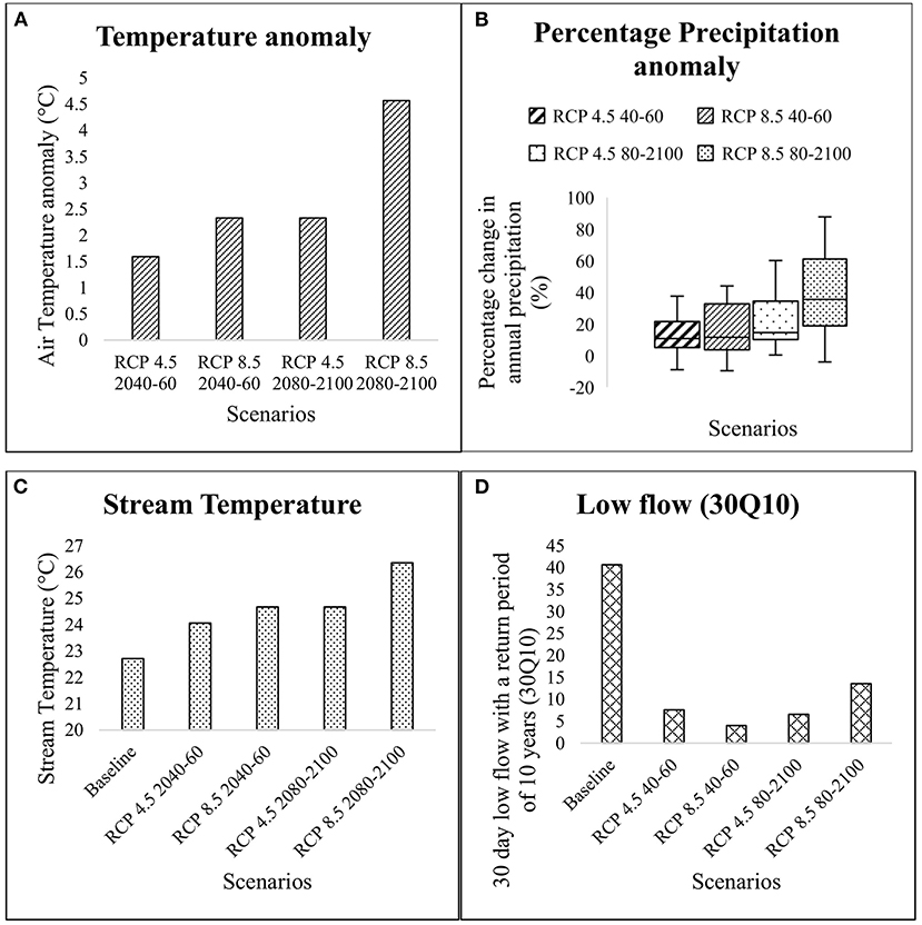
Figure 3. (A) Air temperature anomaly and (B) percentage change in annual precipitation relative to the historical period (1975–2005) for Ankinghat catchment (The horizontal bounding lines of box in box and whisker plot represents the lower and higher quartile and the line inside box represents median) (C) Stream temperature and (D) 30Q10 flow simulated at Ankinghat for climate change scenarios (RCP 4.5 and RCP 8.5) during 2040–2060 and 2080–2100, and the Baseline period (1977–2012).
Stream temperature under warming
The stream temperature simulated for future climate change scenarios from Air-water regression model developed by Santy et al. (2020) for Ankinghat is shown in Figure 3C. The stream temperature increases in the future with time, with a larger increase in temperature corresponding to a larger warming scenario RCP 8.5. The observed increase in river temperature can have an implication on aquatic life, as some organisms won't be able to adapt to the higher temperature (Hari et al., 2006).
Streamflow under warming
The annual and monthly mean streamflow and 30Q10 value for each climate change scenario from the HEC-HMS model are shown in Figure 3D and Supplementary Figure S8. The mean simulated streamflow is not found to vary much for mid-century, while it increases at the end of the twenty-first century (Supplementary Figure S8a). With more warming (in RCP 8.5), streamflow is simulated to rise at the end of the century. The median flow is found to decrease during mid-century in the RCP 8.5 scenario (Supplementary Figure S8a). The median flow is less than the historical flow, and the lowest median flow is simulated for the RCP 8.5 scenario during 2040–60. Peak flow is simulated to increase in future scenarios, with a higher peak flow at the end of the twenty-first century (Supplementary Figure S8a).
The monthly plot of streamflow shows an increase in flows in June and July from the historical period (1977–2012) and a slight increase in January and May months (Supplementary Figure S8b). However, there is a reduction in streamflow in March, April, November, and December. Even though the Ganga River is snow-fed, the barrages constructed upstream nullify the impact of snowmelt on streamflow at Ankinghat, thus having low flows during summer. The lowest flow is observed in March month (Supplementary Figure S8b). The reduction in pre-monsoon flows can reduce the dilution volume for the industrial, municipal sewage, and agricultural pollutant load and hence could lead to a reduction in water quality.
The 30Q10 shows a decline in mid-century, and the lowest 30Q10 is simulated in the RCP 8.5 scenario (Figure 3D). The 30Q10 value increases in the RCP 8.5 scenario at the end of the century. However, all values are less than the historical 30Q10 flow.
Water quality under warming
The water quality parameters are simulated for future climate change scenarios and compared with the baseline period. The water quality profile of (a) DO, (b) BOD, (c) ammonia, (d) nitrate, (e) organic phosphorous, (f) inorganic phosphorous, (g) total nitrogen, (h) total phosphorous, and (i) FC for climate change scenarios RCP 4.5 and RCP 8.5 during 2040–60 and 2080–2100 is shown in Figure 4. The DO is reduced downstream of drain confluence points due to high pollutant concentration inflow to the river (Figure 4A). The DO value decreases with increased pollutant concentration, with the highest sensitivity for BOD, nitrate, and lastly for fecal coliform. The DO concentration is reduced in mid-century, followed by an increase by the end of the twenty-first century for both RCP 4.5 and RCP 8.5 scenarios (Figure 4A). It can also be noticed that DO levels for all scenarios are lower than the baseline value in the mid and end of the twenty-first century. The DO value of Jajmau downstream (critical point) decreases from 5 mg/L in the baseline to 3.8 mg/L for RCP 8.5 2040–60 (Figure 4A). This is because the low flow increases due to increased precipitation in the RCP 8.5 scenario for the end of the twenty-first century. Also, higher temperature yields better reaction kinetics, leading to improved water quality. The least value of DO is simulated in the RCP 8.5 scenario during 2040–60. DO values reach below 4 mgL−1 for ~40 km reach of Kanpur drains downstream in both scenarios, RCP 4.5 and RCP 8.5, making the stretch unfit for aquatic life. A similar reduction of DO with warming is also found in other studies (Cox and Whitehead, 2009; Rehana and Mujumdar, 2012). The increase in stream temperature (Figure 3A) reduces the solubility of oxygen in water and can lead to low values for DO. The increase in stream temperature can also lead to an increased growth rate of phytoplankton and algae, leading to further depletion of DO (Whitehead and Hornberger, 1984; Wade et al., 2002).
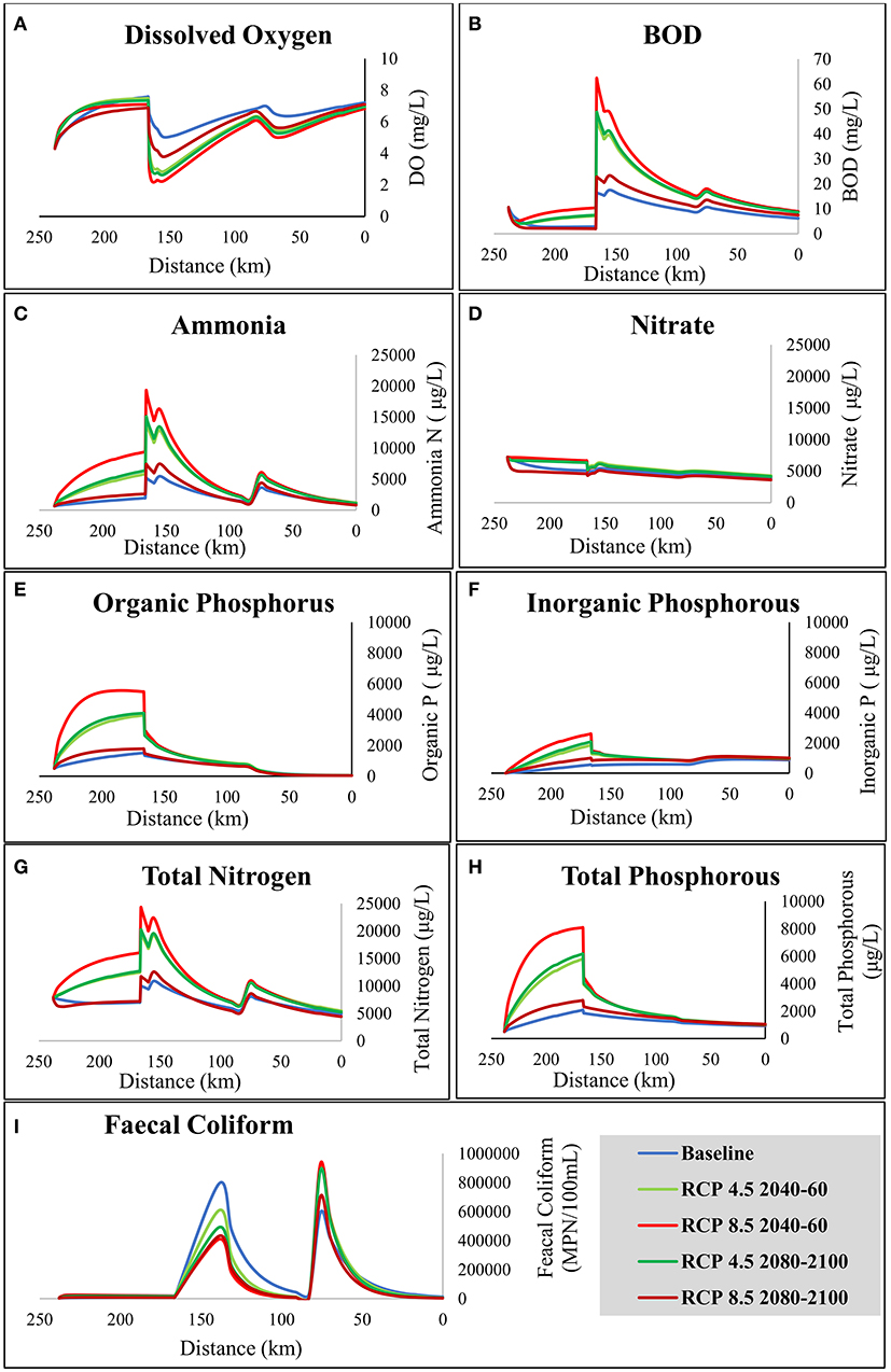
Figure 4. Water quality profile plots of (A) dissolved oxygen (DO), (B) biochemical oxygen demand (BOD), (C) Ammonia, (D) Nitrate, (E) organic-, (F) inorganic phosphorous, (G) Total nitrogen (TN), (H) total phosphorous (TP), and (I) Fecal coliform (FC) for climate change scenarios. The x-axis shows the reach length from Ankinghat (238 km) to Shahzadpur (0 km). Results correspond to low flow events. The lowest values in DO and highest values in BOD, ammonia, nitrate, organic P, inorganic P, TN, TP, and FC correspond to Kanpur, Unnao, Jajmau drains and Pandu river confluence points (Figure 2B). Blue color represents Baseline period; light green and dark green represent the RCP 4.5 scenario during 2040–60 and 2080–2100, respectively, Red and Maroon represent the RCP 8.5 scenario during 2040–60 and 2080–2100, respectively.
Figure 4B shows the BOD profile for RCP 4.5 and RCP 8.5 scenarios. The peaks correspond to the point loads entering the stream. The BOD increases with warming in the mid-century with a higher concentration corresponding to RCP8.5 scenario than in RCP 4.5. The RCP 8.5 scenario shows a low 30Q10, causing an increase in BOD concentration. An increase in BOD of 18–49 mg/L is simulated for Jajmau (highest value) for RCP 8.5 during 2040–60 relative to the baseline (Figure 4B). For mid-century, BOD increases in the RCP 8.5 scenario are larger than in RCP 4.5, while it varies in reverse order for the end of the twenty-first century. The entire river stretch is not fit for bathing, as the BOD value exceeds the prescribed limit of 3 mgL−1. An increase in stream temperature causes an increase in deoxygenation and reaeration rate, with the former dominating the latter downstream of loading points (Santy et al., 2020). The rising stream temperature can also reduce the river's ability to assimilate pollutant loads (Chapra et al., 2021); hence, an increase in BOD is simulated with warming and is confirmed in other studies (Rehana and Mujumdar, 2012; Chapra et al., 2021).
The nutrients considered in the study are ammonia nitrogen, nitrate nitrogen, total nitrogen, organic-, inorganic- and total phosphorous. The nutrient pollution is found to increase with warming in the mid-twenty-first century, while it is found to improve by the end of the twenty-first century compared to the mid-century (Figures 4C–H) following the positive trend in stream flow during low flows. The peaks in the ammonia profile graph and small dips in nitrate correspond to the drain confluence points. Ammonia gets converted to nitrate, and the nitrification process consumes oxygen, leading to depletion of dissolved oxygen in the water (Chapra, 1997). For the climate change scenarios, the highest ammonia concentration of 19.6 mg/L (Figure 4C) is simulated at Kanpur in the RCP 8.5 scenario during 2040–60. Unlike other nutrients, only a slight change in nitrate (0.2–0.6 mg/L rise) (Figure 4D) is simulated with warming because of higher denitrification rate in the Ankinghat-Kanpur stretch (Supplementary Table S6). This result is consistent with Jin et al. (2015), which showed reduced nitrate concentration with climate change in the Thames River. The primary source of nutrient pollution is non-point pollution (Supplementary Tables S1, S8), such as agricultural runoff; however, significant nitrogen compounds are also present in sewage and industrial wastewater reaching the river (Supplementary Table S1).
The concentration of organic phosphorous, inorganic phosphorous, and total phosphorous are shown in Figures 4E,F,H. P concentration increases significantly with warming, with a peak in RCP 8.5 during 2040–60, corresponding to low flow and less dilution volume. Unlike other pollutants, the primary source of phosphorous pollution is non-point sources (Supplementary Tables S1, S8), mainly fertilizers. The only P load-carrying drain is the Jajmau drain (Supplementary Table S1). The loading is highest in the Ankinghat to Kanpur reach. A reduction in P concentration is found at drain confluence due to the absence of P concentration from drains which acts as dilution water. The organic P, inorganic P, and TP concentration vary with warming in the same order as other water quality parameters considered here. The total phosphorus concentration is found to increase from 1.8 mg/L in the baseline to 4.5 mg/L in the RCP 8.5 scenario during 2040–60 (Figure 4H). Phosphorus concentration is also found to increase in the future in another study on the Ganga river with a business as usual scenario (Jin et al., 2015). There is an increase in river pollution in future climate change scenarios, mainly due to the rise in stream temperature and reduction in low flows, which affect the kinetics and dilution factors. The entire stretch falls in the trophic state 'Eutrophic' as total phosphorous concentration exceeds the limits of 20 μgP/L throughout the stretch (Chapra, 1997). Low flows can enhance the chances of eutrophication in rivers due to a reduction of DO (Bocaniov et al., 2016). The rise in population and agriculture can lead to more P loading in the future. However, our study focuses only on isolating the effects of climate change on water quality; therefore, other factors such as point loads, agricultural runoff, population, and industrialization will remain unchanged.
Figure 4I shows the fecal coliform (FC) profile for RCP 4.5 and 8.5 scenarios. The high concentration of FC throughout the stretch shows the presence of raw sewage without treatment in the river. The peaks in the plot correspond to Jajmau drains d/s and Pandu River confluence d/s, where a high FC load joins the river. The entire stretch is not suitable for bathing as it exceeds its limit of 500 MPN/100 mL. This high concentration of FC indicates the need for more sewage treatment plants for the stretch. The FC is found to decrease in the RCP 4.5 scenario for both time slices, while it increases in RCP 8.5. Highest FC concentration (9,91,139 MPN/100 mL) at Jajmau is simulated in RCP 8.5 during 2040–60 (Figure 4I). Jajmau and Fatehpur are the most affected checkpoints for FC. There is a slight reduction in FC concentration for the downstream stretch of Pandu River confluence from mid to end of the twenty-first century in RCP 4.5, while there is a drastic reduction in RCP 8.5. This reduction can be attributed to higher reaction kinetics in warmer conditions. At Kanpur and Shahzadpur also, similar patterns are simulated. The lowermost FC value for the stretch is at headwater (3,300 MPN/100 mL). FC is gradually increasing up to Kanpur drains due to non-point source pollution, but we can see that FC pollution from drains is high (~102 times) compared to non-point source pollution (Supplementary Tables S1, S8). The varied trend of FC with climate change at different locations is due to the varied sensitivity of FC to temperature and streamflow throughout the stretch (Santy et al., 2020). A reduction of fecal coliform with warming has been also simulated for Lis River, Portugal in a past study (Fonseca et al., 2014).
The pollution hotspots identified in the stretch are Kanpur and Jajmau (Figure 4), and the percentage change for each water quality parameter for the worst-case climate change scenario (RCP 8.5 during 2040–60) is shown in Figure 5A and for other scenarios in Supplementary Figure S9. The water quality parameter most affected by future climate change scenarios simulated is BOD and ammonia nitrogen; however, all parameters considered have a significant change due to warming.
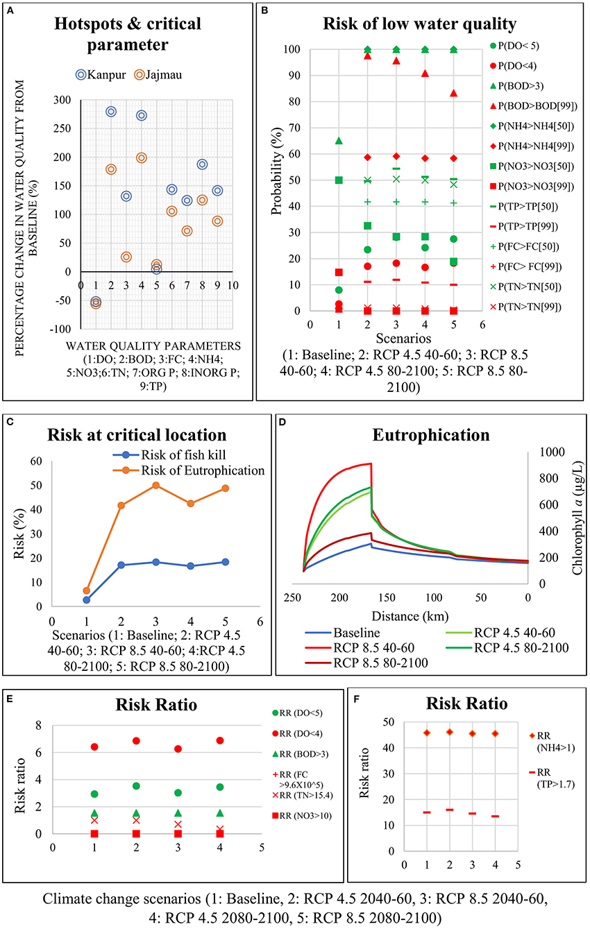
Figure 5. Hotspot identification, eutrophication profile and risk plots. (A) Percentage change in water quality parameters for the critical climate change scenario (RCP 8.5 40–60) from Baseline period; (B) Risk of low water quality in terms of all parameters at Kanpur. Circle, triangle, diamond, square, minus and plus symbols represent dissolved oxygen, biochemical oxygen demand, ammonia, nitrate, total phosphorous and fecal coliform, respectively; Two thresholds are adopted for risk calculation, with smaller threshold shown in green color and higher threshold in red color (Table 2). The numbers written in square bracket represents the percentile value of Baseline period considered; (C) Risk of fish kill (blue) and eutrophication (orange) at critical location Jajmau; (D) Chlorophyll a profile for all scenarios considered during low flow; (E) Risk ratio of DO (with aquatic and bathing limits), BOD, fecal coliform, nitrate, and total nitrogen for the future climate change scenarios; (F) Risk ratio of ammonia and total phosphorous for future climate change scenarios.
Risk of reduced water quality
A boxplot of water quality for the entire period of the Baseline, RCP 4.5 2040–2060, RCP 8.5 2040–2060, RCP 4.5 2080–2100, and RCP 8.5 2080–2100 scenarios is shown in Supplementary Figure S10. The thresholds selected for the risk analysis are listed in Table 2. The maximum values of pollutant concentration in the historical period are often used as design values for water quality studies (Ahmad and Schroeder, 2003; Chouinarda et al., 2014; Berkessa et al., 2019). Hence extreme water quality statistics (99th percentile values) of the water quality parameters in the baseline period are selected as the thresholds for BOD, ammonia, total nitrogen, and total phosphorous. The median of the baseline period is also considered as another threshold to analyze the changes in median concentration for future. The risk of low water quality for individual water quality parameters, DO, BOD, ammonia, nitrate, total nitrogen, total phosphorous, and fecal coliform calculated from the frequency analysis of time series data for each scenario is shown in Figure 5B.
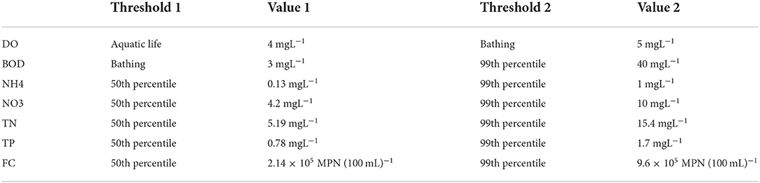
Table 2. Thresholds adopted for risk calculation (Percentile calculation is carried out from Baseline data).
The risk of low DO, with two thresholds, 4 mg L−1 (aquatic life limits) and 5 mg L−1 (bathing class limits), indicates that river is unfit for aquatic life and bathing for a more extended period in the future than in the baseline period. The risk of low DO concentration with bathing class limit increases from 8% in baseline to 28% in RCP 8.5 during 2040–60 (Figure 5B). Both the frequency and intensity of low DO events increase in future due to warming, which can be attributed to more low flow or droughts in future (Supplementary Figure S11). Reduced saturation DO, and less dilution volume with the same point loads and non-point loads result in reduced DO during low-flow periods in the future. Thus, increasing the frequency and duration of the low-flow periods in a warmer world could increase the risk of reduced water quality.
The increase in risk of high BOD for future shows the intensification of organic pollution in the future (Figure 4B). The risk of BOD > 3 mg L−1 (the bathing class limit) has increased from 65 to 100% in the future indicating the river is highly polluted with warming. The risk of BOD > 40 mg L−1 is calculated to highlight the intensification of magnitude and the trend. The risk peaks during the 2040–60 period and then slightly decrease in 2080–2100. Here we see a contradicting trend with warming scenarios for BOD, where the risk is more in RCP 4.5 scenario (Figure 5B) despite higher BOD in the RCP 8.5 scenario in low flow events (Figure 4B). This shows that organic pollution is critical not only in low flow events but also in high flows.
The risk of microbial pollution has slightly reduced with warming (Figure 5B) because of larger pathogen decay rates at higher temperatures; however, the concentration is very high than the bathing limits. The risk of microbial pollution reduces from 50% in baseline to 42% in RCP 8.5 2040–60 (Figure 5B). The risk of nutrient pollution (TN and TP) increases in the mid-twenty-first century and then reduces by the end of the century following the reduction in the frequency of low-flows events. The nitrogen components show a mixed response, with an increased risk of ammonia and decreased risk of nitrate in the future (Figure 5B). The risk of ammonia pollution increases from 1% in baseline to 59% in RCP 8.5 during 2040–60 (Figure 5B). Nitrate concentration shows a slight (decrease in RCP 8.5 during 2080–2100 and increase for other scenarios) change even in the critical low flow period for the future, and for other flows with high dilution volume, nitrate concentration decreases, resulting in the reduction of its risk in the future.
The risk of extreme nitrate pollution in the future is found to be reduced to zero from 15% in the baseline (Figure 5B). The risk of nitrate pollution reduces with warming, especially at the end of the twenty-first century because, even for the critical low flow period, there is small reduction in the nitrate concentration of the river (Figure 4D). For other flows with high dilution volume, nitrate concentration decreases (Supplementary Figure S10d), resulting in reducing its risk in the future. Overall reduction of nitrate has also been found with warming in other studies (Whitehead et al., 2015b). Further, we find that total phosphorous risk increases with warming due to an increased frequency of low flow periods simulated for the future. An increase in extreme total phosphorus risk from 0.7% in baseline to 12% in RCP 8.5 during 2040–60 is simulated (Figure 5B). The increased risk of nutrient pollution can lead to increased eutrophication (Figure 5C) due to a higher chlorophyll a value in the future (Figure 5D).
The risk ratio calculated for the future climate change scenarios is shown in Figures 5E,F. The water quality parameters FC and nitrate have an RR value below 1 for all scenarios indicating a decreased risk for the future. The RR value of total nitrogen is near 1 for mid-century, while it falls below one at the end of the century following a reduction in nitrate concentration with warming. The RR value for DO, BOD, ammonia and total phosphorous is >1, indicating an increased risk for the future (Figure 5E; Supplementary Figure S12).
Risk of eutrophication
The risk of eutrophication calculated from the chlorophyll a value for the hotspot Jajmau is shown in Figure 5C. The entire stretch is eutrophic for the Baseline; hence the 95th percentile chlorophyll a value is taken as the threshold for risk calculation. A significant increase in eutrophication is found at Jajmau with warming increased TP concentration. An increase in risk of eutrophication from 6.5% in baseline to 50% in the mid-twenty-first century is simulated with climate change (Figure 5C). The reduction in summer flow rates could increase residence time and, hence, enhance algae growth. Also, increased residence time could reduce the turbidity, allowing sedimentation, increased light penetration, and increased algae growth (Whitehead and Hornberger, 1984; Whitehead et al., 2009). Land use land cover would also play a role in eutrophication due to changes in agricultural runoff. In this study, we have assumed the non-point source load to remain constant, as our objective is to quantify the individual contribution of climate change to eutrophication. Risk of eutrophication peaks for RCP 8.5 during 2040–60, which corresponds to the scenario with more low flow events. However, the change from mid-century to the end of the century is not significant.
Risk of fish kill
The risk of fish kill calculated from DO of the river at the hotspot location shows an increased risk (Figure 5C) in future due to more low DO events in future. In the baseline period, DO is above 4 mg L−1 even at critical locations, while for climate change scenarios DO falls below 4 mg L−1 in the low flow period due to warming (Figure 4A). An increase in risk of fish kill from 3% in baseline to 18% in mid-twenty-first century is simulated with climate change (Figure 5C). The occurrence of low DO associated with low flow events are more frequent in the future, and hence fish kill is more likely to happen with future warming. The largest risk corresponds to the RCP8.5 scenario during 2040–60. Thus, the trend of fish kill also follows the same trend of DO with warming, with most critical value in mid-century which improves by the end of century. A large number of fish death have also been reported with increased warming in previous studies (Gunn, 2002).
Conclusion
After launching the Ganga Action Plan in 1986 (Environment Forests Division Water Resources Division Planning Commission Government of India, 2009), the Indian government is currently taking measures to clean up the Ganga River. In this paper, an investigation is carried out to analyze the isolated effects of climate change on water quality and to calculate the risk of reduced water quality, eutrophication and fish kill using a coupled hydrological (HEC-HMS) and water quality simulation model (QUAL2K). Statistically downscaled climate projections are used to drive coupled HEC-HMS—QUAL2K model framework.
It is found that water quality is likely to be reduced in the mid-twenty-first century (2040–2060), with a slight improvement by the end of twenty-first century (2080–2100). The projected increase in pre-monsoon precipitation would result in an increase in low flows in the 2080–2100 compared to 2040–60, hence, relatively better water quality is simulated toward the end of twenty-first century in association with an increase in dilution volume. The pollution hotspots identified in the reach stretch considered in this study are Kanpur and Jajmau, due to large upstream pollution load from Kanpur, Unnao and Jajmau drain. The most affected water quality parameters with warming are BOD and ammonia nitrogen. The entire stretch of the study area is simulated to be eutrophic from large total phosphorous and chlorophyll a which are already near the limits in the baseline period. The concentrations of phosphorous and chlorophyll a further increase with warming. It is found that climate change alone can result in a deterioration of water quality in the future with a percentage increase in nutrients and BOD by more than 50% from baseline.
The frequency analysis approach shows an increased risk of reduced DO and increased risk of enhanced organic (BOD), ammonia and nutrient (total nitrogen and total phosphorous) pollution in the future with warming. However, reduced risk of nitrate and microbial pollution is simulated for the future with an overall reduction in nitrate and fecal coliform concentration due to increased nitrate denitrification rate and pathogen decay rate with temperature. The risk of eutrophication for low flow periods calculated from chlorophyll a concentration significantly increases with warming. The increased risk of eutrophication is due to an increase in total phosphorous because of a reduction of low flows, which causes less dilution. The risk of fish kill is calculated from the river's dissolved oxygen by taking Indian standard DO limits for maintenance of aquatic life as the threshold. The risk is likely to increase in the future, with peaks in mid-century and a slight reduction in risk by the end of the century. The increase in risk from baseline is due to more low DO events associated with more low flows simulated for the future. The risk of eutrophication and fish kill is likely to increase by 43.5 and 15% by the mid twenty-first century due to climate change alone.
Our study is likely to be beneficial for policy makers and governing authorities for taking appropriate actions to control Ganga River pollution. However, there are some limitations to our study. For instance, the risk of eutrophication is calculated based on chlorophyll a value calculated using an empirical equation. As this equation is not initially developed for Indian conditions, its application here likely introduces some uncertainty. The risk of fish kill is quantified by taking threshold of DO at 4 mg L−1, the limits given by pollution control board, India. However, the threshold of DO for different fish species differ (Hoff, 1967) and hence if the risk of fish kill of a particular species is needed, the corresponding thresholds should be adopted. The point loads from drains are assumed to be constant in the future, however, this is subjected to change in the future due to the steps taken by the government in cleaning Ganga River. Further, model uncertainty and parameter uncertainty bring in some amount of uncertainty to our results which could be narrowed down by performing similar risk estimates using various hydrological and water quality models. The risk of reduced water quality with other pollution drivers such as land use and land cover change, enhanced agricultural and industrial activities, population growth, and the corresponding growth in sewage treatment facilities would be the subject of a future study. Quantification of water quality changes during the monsoon season and extreme flow events for this stretch of the Ganga River also merits investigation in the future.
Data availability statement
The data that support the findings of this study are available from Ministry of Water Resources, Government of India but restrictions apply to the availability of these data, which were used under license for the current study, and so are not publicly available. Requests to access these datasets should be directed to http://www.cwc.gov.in.
Author contributions
SS developed the model, made computational runs, and prepared first draft of the manuscript including figures. PM conceptualized the model, facilitated data collection, and edited the manuscript. GB helped in devising climate change scenarios and review of manuscript. All authors contributed to the article and approved the submitted version.
Funding
The funding was received from the Ministry of Earth Sciences (MoES), Government of India, through the Project, Advanced Research in Hydrology and Knowledge Dissemination, Project No. MOES/PAMC/H&C/41/2013-PCII and the Department of Science and Technology (DST), India through the Project No. DST/NSM/R&D_HPC_Applications/2021/03.09. PM acknowledges the support received through the JC Bose Fellowship (Number, JCB/2018/000031).
Acknowledgments
We thank the Chief Engineer, Upper Ganga Basin Organization, Central Water Commission, Lucknow for providing very useful data on streamflow, water quality, and hydraulic characteristics for the river stretch studied, India Meteorological Department for providing temperature data, National Remote Sensing Center, Hyderabad for providing us land use land cover data. United States Geological Survey for providing DEM data, the European Center for Medium-Range Weather Forecasts for providing atmospheric data and NASA Center for Climate Simulation for providing NASA Earth Exchange Global Daily Downscaled Climate Projections. We also thank the Divecha Center for Climate Change, IISc, Bangalore for providing Grantham Fellowship to SS. The authors are thankful to Dr. Pankaj Dey for the help with proof reading the manuscript.
Conflict of interest
The authors declare that the research was conducted in the absence of any commercial or financial relationships that could be construed as a potential conflict of interest.
Publisher's note
All claims expressed in this article are solely those of the authors and do not necessarily represent those of their affiliated organizations, or those of the publisher, the editors and the reviewers. Any product that may be evaluated in this article, or claim that may be made by its manufacturer, is not guaranteed or endorsed by the publisher.
Supplementary material
The Supplementary Material for this article can be found online at: https://www.frontiersin.org/articles/10.3389/frwa.2022.971623/full#supplementary-material
Abbreviations
30Q10, 30 day low flow with a return period of 10 years; BOD, Biochemical Oxygen Demand; Chla, Chlorophyll a; CPCB, Central Pollution Control Board; DO, Dissolved Oxygen; FC, Fecal coliform; GAP, Ganga Action Plan; IIT, Indian Institute of Technology; IS, Indian Standards; JD, Jajmau drain; KD, Kanpur drain; P, Phosphorous; PD, Pandu river drain; RR, Risk ratio; TN, Total nitrogen; TP, Total Phosphorous; UD, Unnao drain.
References
Adamovich, B. V., Medvinsky, A. B., Nikitina, L. V., Radchikova, N. P., Mikheyeva, T. M., Kovalevskaya, R. Z., et al. (2019). Relations between variations in the lake bacterioplankton abundance and the lake trophic state: evidence from the 20-year monitoring. Ecol. Indic. 97, 120–129. doi: 10.1016/j.ecolind.2018.09.049
Ahmad, S., and Schroeder, R. G. (2003). The impact of human resource management practices on operational performance: recognizing country and industry differences. J. Operat. Manag. 21, 19–43. doi: 10.1016/S0272-6963(02)00056-6
Austin, B. (1998). The effects of pollution on fish health. J. Appl. Microbiol. 85(Suppl. 1), 234S−242S. doi: 10.1111/j.1365-2672.1998.tb05303.x
Barbarossa, V., Bosmans, J., Wanders, N., King, H., Bierkens, M. F. P., Huijbregts, M. A. J., et al. (2021). Threats of global warming to the world's freshwater fishes. Nat. Commun. 12, 1701. doi: 10.1038/s41467-021-21655-w
Bartsch, A. F., and Gakstatter, J. H. (1978). “Management decisions for lake sysytems on a survey of trophic status, limiting nutrients and nutrients loadings,” in American - Soviet Symposium on Use of Mathematical Models to Optimize Water Quality Management (Gulf Breeze, FL: U. S EPA Office of Research and Development), 374–394.
Bennett, T. (1998). Development and application of a continuous soil moisture accounting algorithm for the hydrologic engineering center hydrologic modeling system (HEC-HMS). (MS thesis). Dept. of Civil and Environmental Engineering, University of California, Davis, Davis, CA, USA.
Berkessa, Y. W., and Mereta, S. T., and Feyisa, F. F. (2019). Simultaneous removal of nitrate and phosphate from wastewater using solid waste from factory. Appl. Water Sci. 9, 28. doi: 10.1007/s13201-019-0906-z
Bharati, L., Lacombe, G., Gurung, P., Jayakody, P., Hoanh, C. T., Smakhtin, V., et al. (2011). The Impacts of Water Infrastructure and Climate Change on the Hydrology of the Upper Ganges River Basin. Colombo: International Water Management Institute, 36. (IWMI Research Report 142).
Bocaniov, S. A., Leon, L. F., Rao, Y. R., Schwab, D. J., and Scavia, D. (2016). Simulating the effect of nutrient reduction on hypoxia in a large lake (Lake Erie, USA-Canada) with a three-dimensional lake model. J. Great Lakes Res. 42, 1228–1240. doi: 10.1016/j.jglr.2016.06.001
Bouraoui, F., and Galbiati, L., and Bidoglio, G. (2002). Climate change impacts on nutrient loads in the Yorkshire Ouse catchment (UK). Hydrol. Earth Syst. Sci. 6, 197–209. doi: 10.5194/hess-6-197-2002
Bristow, K. L., and Campbell, G. S. (1984). On the relationship between incoming solar radiation and daily maximum and minimum temperature. Agric. Forest Meteorol. 31, 159–166. doi: 10.1016/0168-1923(84)90017-0
Carlson, R. E. (1991). Expanding the trophic state concept to identify non-nutrient limited lakes and reservoirs. Enhancing States's Lake Manag. Prog. 59–71.
Carmichael, J. J., Strzepek, K. M., and Minarik, B. (1996). Impacts of climate change and seasonal variability on economic treatment costs: a case study of the Nitra River Basin, Slovakia. Water Resour. Dev. 12, 209–227. doi: 10.1080/07900629650041966
Caruso, B. (2002). Temporal and spatial patterns of extreme low flows and effects on stream ecosystems in Otago, New Zealand. J. Hydrol. 257, 115–133. doi: 10.1016/S0022-1694(01)00546-7
Central Pollution Control Board (2013). Pollution Assessment: River Ganga (CPCB 2013). New Delhi: Central Pollution Control Board.
Central Water Commission and National Remote Sensing Centre (2014). Ganga Basin. New Delhi: Government of India Ministry of Water Resources.
Chapra, S. C., Camacho, L. A., and McBride, G. B. (2021). Impact of global warming on dissolved oxygen and BOD assimilative capacity of the world's rivers: modeling analysis. Water 13, 2408. doi: 10.3390/w13172408
Chapra, S. C., and Pelletier, G. J. (2003). QUAL2K: A Modeling Framework for Simulating River and Stream Water Quality: Documentation and User's Manual. Medford, MA: Civil and Environmental Engineering Dept., Tufs University.
Chaudhary, S., Dhanya, C. T., Kumar, A., and Shaik, R. (2019). Water quality–based environmental flow under plausible temperature and pollution scenarios. J. Hydrol. Eng. 24, 1780. doi: 10.1061/(ASCE)HE.1943-5584.0001780
Chouinarda, A., Balch, G. C., Wootton, B. C., Jørgensen, S. E., and Anderson, B. C. (2014). Chapter 19 - subwet 2, 0. Modeling the performance of treatment wetlands. Dev. Environ. Model. 26, 519–537. doi: 10.1016/B978-0-444-63249-4.00021-X
Chow, V. T., Maidment, D. R., and Mays, L. W. (1988). Applied Hydrology. New York, NY: McGraw-Hill Book Company.
Consortium of 7 “Indian Institute of Technology” s (IITs) (2013). Ganga River Basin Environment Management Plan: Interim Report. New Delhi: IITs.
Cox, B. A., and Whitehead, P. G. (2009). Impacts of climate change scenarios on dissolved oxygen in the River Thames, UK. Hydrol. Res. 40, 138–152. doi: 10.2166/nh.2009.096
Davids, J. C., Rutten, M. M., Shah, R. D. T., Shah, D. N., Devkota, N., Izeboud, P., et al. (2018). Quantifying the connections—linkages between land-use and water in the Kathmandu, Valley Nepal. Environ. Monit. Assess. 190, 304. doi: 10.1007/s10661-018-6687-2
Ding, C. Z., Jiang, X. M., Chen, L. Q., Juan, T., and Chen, Z. M. (2016). Growth variation of Schizothorax dulongensis Huang, 1985 along altitudinal gradients: implications for the Tibetan Plateau fishes under climate change. J. Appl. Icthyol. 32, 729–733. doi: 10.1111/jai.13102
Dodds, W. K., and Whiles, M. R. (2020). Chapter 12 - aquatic chemistry and factors controlling nutrient cycling: redox and O2. Fresh. Ecol. Aquat. Ecol. 335–369. doi: 10.1016/B978-0-12-813255-5.00012-0
Ducharne, A., Baubion, C., Beaudoin, N., Benoît, M., Billen, G., Brisson, N., et al. (2006). 2007 Long term prospective of the Seine River system: confronting climatic and direct anthropogenic changes. Sci. Total Environ. 375, 292–311. doi: 10.1016/j.scitotenv.2006.12.011
Dyer, F., ElSawah, S., Croke, B., Griffiths, R., Harrison, E., Lucena-Moya, P., et al. (2014). The effects of climate change on ecologically-relevant flow regime and water quality attributes. Stoch Environ. Res. Risk Assess 28, 67–82. doi: 10.1007/s00477-013-0744-8
Edwards, M., Johns, D. G., Leterme, S. C., Svendsen, E., and Richardson, A. J. (2006). Regional climate change and harmful algal blooms in the northeast Atlantic. Limnol. Oceanogr. 51, 820–829. doi: 10.4319/lo.2006.51.2.0820
Environment and Forests Division and Water Resources Division Planning Commission Government of India (2009). Report on Utilisation of Funds and Assets Created Through Ganga Action Plan in States Under GAP. New Delhi: Environment and Forests Division and Water Resources Division Planning Commission Government of India.
Ficklin, D. L., Stewart, I. T., and Maurer, E. P. (2013). Effects of climate change on stream temperature, dissolved oxygen, and sediment concentration in the Sierra Nevada in California. Water Resour. Res. 49. 2765–2782. doi: 10.1002/wrcr.20248
Fleming, M. (2002). Continuous hydrologic modeling with HMS: parameter estimation and model calibration and validation. (MS thesis). Dept. of Civil and Environmental Engineering, Tennessee Technological Univ., Cookeville, Tenn, USA.
Fonseca, A., Botelho, C., Boaventura, R. A. R., and Vilar, V. J. P. (2014). Global warming effects on faecal coliform bacterium watershed impairments in Portugal. River Res. Appl. 31, 1344–1353. doi: 10.1002/rra.2821
Gittings, J. A., Raitsos, D. E., Krokos, G., and Hoteit, I. (2018). Impacts of warming on phytoplankton abundance and phenology in a typical tropical marine ecosystem. Sci. Rep. 8, 2240. doi: 10.1038/s41598-018-20560-5
Gunn, J. M. (2002). Impact of 1998 El Nino event on a lake charr, Salvelinus namaycush, population recovering from acidification. Environ. Biol. Fish 64, 343–351. doi: 10.1023/A:1016058606770
Gyawali, S., Techato, K., Monprapussorn, S., and Yuangyai, C. (2013). Integrating land use and water quality for environmental based land use planning for U-tapao River Basin. Thailand. Procedia Soc. Behav. Sci. 91, 556–563. doi: 10.1016/j.sbspro.2013.08.454
Hansson, L. A., and Brönmark, C. (2009). Biomanipulation of aquatic ecosystems. Encyclopedia of Inland waters. Ref. Module Earth Syst. Environ. Sci. Encycl. Inland Waters 242–248. doi: 10.1016/B978-012370626-3.00240-4
Hari, R., Livingstone, D., Siber, R., Burkhardt-Holm, P., and Güttinger, H. (2006). Consequences of climatic change for water temperature and brown trout populations in Alpine rivers and streams. Global Change Biol. 12, 10–26. doi: 10.1111/j.1365-2486.2005.001051.x
Held, I. M., and Soden, B. J. (2006). Robust responses of the hydrological cycle to global warming. J. Clim. 19, 5686–5699. doi: 10.1175/JCLI3990.1
Hoff, J. G. (1967). Lethal oxygen concentration for three marine fish species. J. Water Pollut Control Fed. 39, 267–77.
Jacobs, S. R., Weeser, B., Guzha, A. C., Rufino, M. C., Butterbach-Bahl, K., Windhorst, D., et al. (2018). Using high-resolution data to assess land use impact on nitrate dynamics in East African Tropical Montane Catchments. Water Resour. Res. 54, 1812–1830. doi: 10.1002/2017WR021592
Jain, C. K., and Singh, S. (2018). Impact of climate change on the hydrological dynamics of River Ganga, India. J. Water Clim. Change 11, 274–290. doi: 10.2166/wcc.2018.029
Javadinejad, S., Eslamian, S., and Ostad-Ali-Askari, K. (2021). The analysis of the most important climatic parameters affecting performance of crop variability in a changing climate. Int. J. Hydrol. Sci. Technol. (IJHST). 11, 1. doi: 10.1504/IJHST.2021.112651
Jin, L., Whitehead, P. G., Sarkar, S., Sinha, R., Futter, M. N., Butterfield, D., et al. (2015). Assessing the impacts of climate change and socio-economic changes on flow and phosphorus flux in the Ganga river system. Environ. Sci. Proc. Impacts 17, 1098–1110. doi: 10.1039/C5EM00092K
Johnk, K. D., Huisman, J., Sharples, J., Sommeijer, B., Visser, P. M., Stroom, J. M., et al. (2008). Summer heatwaves promote blooms of harmful Cyanobacteria. Glob. Chang Biol. 14, 495–512. doi: 10.1111/j.1365-2486.2007.01510.x
Khan, M. Y. A., Gani, K. M., and Chakrapani, G. J. (2017). Spatial and temporal variations of physicochemical and heavy metal pollution in Ramganga River—a tributary of River Ganges, India. Environ. Earth Sci. 76, 231. doi: 10.1007/s12665-017-6547-3
Khattiyavong, C., and Lee, H. S. (2019). Performance Simulation an assessment of an appropriate wastewater treatment technology in a densely populated growing City in a developing country: a case study in Vientiane, Laos. Water 11, 1012. doi: 10.3390/w11051012
Kibria, G. (2014). Global Fish Kills; Causes and Consequences. Available online at: https://www.researchgate.net/publication/261216309_Global_fish_Kills_Causes_and_Consequences/citation/download (accessed October 5, 2021).
Kosten, S., Huszar, V. L., Bécares, E., Costa, L. S., van Donk, E., and Hansson, L. A., et al. (2011). Warmer climate boosts cyanobacterial dominance in shallow lakes. Glob. Change Biol. 18, 118–126. doi: 10.1111/j.1365-2486.2011.02488.x
Liu, Y., Zhang, J., and Zhao, Y. (2018). The risk assessment of river water pollution based on a modified non-linear model. Water 10, 362. doi: 10.3390/w10040362
Matthews, R., Hilles, M., and Pelletier, G. (2002). Determining trophic state in Lake Whatcom, Washington (USA), a soft water lake exhibiting seasonal nitrogen limitation. Hydrobiologia 468, 107–121. doi: 10.1023/A:1015288519122
Mortazavi-Naeini, M., Bussi, G., Elliott, J. A., Hall, J. W., and Whitehead, P. G. (2019). Assessment of risks to public water supply from low flows and harmful water quality in a changing climate. Water Resour. Res. 55, 386–10.404. doi: 10.1029/2018WR022865
Mujumdar, P. P., and Sasikumar, K. (2002). A fuzzy risk approach for seasonal water quality management of a river system. Water Resour. Res. 38, 5-1–5-9. doi: 10.1029/2000WR000126
Namugizea, J. N., Jewitta, G., and Graham, M. (2018). Effects of land use and land cover changes on water quality in the uMngeni river catchment, South Africa. Phys. Chem. Earth 105, 247–264. doi: 10.1016/j.pce.2018.03.013
National River Conservation Directorate and Ministry of Environment and Forests (2009). Status Paper on River Ganga State of Environment and Water Quality. New Delhi: Alternate Hydro Energy Centre, Indian Institute of Technology Roorkee.
Nazari-Sharabian, M., Ahmad, S., and Karakouzian, M. (2018). Climate change and eutrophication: a short review. Eng. Technol. Appl. Sci. Res. 8, 3668–3672. doi: 10.48084/etasr.2392
Ostad-Ali-Askari, K. (2022). Management of risks substances and sustainable development. Appl. Water Sci 12, 65. doi: 10.1007/s13201-021-01562-7
Ostad-Ali-Askari, K., Shayannejad, M., and Ghorbanizadeh-Kharazi, H. (2017). Artificial neural network for modeling nitrate pollution of groundwater in marginal area of Zayandeh-rood River, Isfahan, Iran. KSCE J. Civ. Eng. 21, 134–140. doi: 10.1007/s12205-016-0572-8
Peperzak, L. (2003). Climate change and harmful algal blooms in the North Sea. Acta Oecol. 24, 139–144. doi: 10.1016/S1146-609X(03)00009-2
Permatasari, P. A., Setiawan, Y., Khairiah, R. N., and Effendi, H. (2017). The effect of land use change on water quality: a case study in Ciliwung Watershed. IOP Conf. Ser. Earth Environ. Sci. 54, 012026. doi: 10.1088/1755-1315/54/1/012026
Perry, A. L., Low, P. J., Ellis, J. R., and Reynold, J. D. (2005). Climate change and distribution shifts in marine fishes. Science 308, 1912–1915. doi: 10.1126/science.1111322
Rehana, S., and Mujumdar, P. P. (2011). River water quality response under hypothetical climate change scenarios in Tunga-Bhadra river, India. Hydrol. Proc. 25, 3373–3386. doi: 10.1002/hyp.8057
Rehana, S., and Mujumdar, P. P. (2012). Climate change induced risk in water quality control problems. J. Hydrol. 444–445, 63–77. doi: 10.1016/j.jhydrol.2012.03.042
Saha, A., and Ghosh, S. (2020). Relative impacts of projected climate and land use changes on terrestrial water balance: a case study on ganga river Basin. Front. Water Sec. Water Built Environ. 2, 12. doi: 10.3389/frwa.2020.00012
Sahu, S., Pyasi, S. K., and Galkate, R. V. (2020). A review on the HEC-HMS rainfall-runoff simulation model. Int. J. Agric. Sci. Res. 10, 183–190. doi: 10.24247/ijasraug202024
Salvi, K., Kannan, K. S., and Ghosh, S. (2011). “Statistical downscaling and bias correction for projections of indian rainfall and temperature in climate change studies,” International Conference on Environmental and Computer Science IPCBEE, Vol. 19. Singapore: IACSIT Press.
Santy, S., Mujumdar, P. P., and Bala, G. (2020). Potential impacts of climate and land use change on the water quality of ganga river around the industrialized Kanpur region. Sci. Rep. 10, 9107. doi: 10.1038/s41598-020-66171-x
SCS. (1986). Urban Hydrology for Small Watersheds. Tech. Release No. 55, Soil Conservation Service. Washington, DC: USDA.
Shayannejad, M., Ghobadi, M., and Ostad-Ali-Askari, K. (2022). Modeling of surface flow and infiltration during surface irrigation advance based on numerical solution of saint–venant equations using Preissmann's scheme. Pure Appl. Geophys. 179, 1103–1113. doi: 10.1007/s00024-022-02962-9
Skaggs, R. W., and Khaleel, R. (1982). “Hydrologic modeling of small watersheds,” in An ASAE Monograph Number 5 in a Series, eds C. T. Haan, H. P. Johnson, and D. L. Brakenstek (New York, NY: American Society of Agricultural Engineers).
Tao, J., He, D. K., Kennard, M. J., Ding, C. Z., Bunn, S. E., Liu, C. L., et al. (2018). Strong evidence for changing fish reproductive phenology under climate warming on the Tibetan Plateau. Glob. Change Biol. 24, 2093–2104. doi: 10.1111/gcb.14050
Tedesco, P. A., Oberdorff, T., Cornu, J. F., Beauchard, O., Brosse, S., Durr, H. H., et al. (2013). A scenario for impacts of water availability loss due to climate change on riverine fish extinction rates. J. Appl. Ecol. 50, 1105–1115. doi: 10.1111/1365-2664.12125
Ueda, H., Iwai, A., Kuwako, K., and Hori, M. E. (2006). Impact of anthropogenic forcing on the Asian summer monsoon as simulated by eight GCMs. Geophys. Res. Lett. 33, L06703. doi: 10.1029/2005GL025336
U. S. Army Corps of Engineers Hydrologic Engineering Center (2000). Hydrologic Modeling System HEC-HMS Technical Reference Manual. Davis, CA: U. S. Army Corps of Engineers Hydrologic Engineering Center.
Uttar Pradesh Jal Nigam, Uttar Pradesh Pollution Control Board, National Mission for Clean Ganga, MoWR, RD & GR, Central Pollution Control Board, and MoEF&CC. (2016). Assessment of Pollution of Drains Carrying Sewage/Industrial Effluent Joining River Ganga and its Tributaries (Kali-East/Ramganga) Between Haridwar (Down) to Kanpur (Down). New Delhi: National Green Tribunal Principal Bench.
Wade, A. J., Whitehead, P. G., Hornberger, G. M., and Snook, D. L. (2002). On modelling the flow controls on macrophyte and epiphyte dynamics in a lowland permeable catchment: the River Kennet, southern England. Sci. Total Environ. 282–283, 375–393. doi: 10.1016/S0048-9697(01)00925-1
Walker, J. W. W. (1979). Use of hypolimnetic oxygen depletion rate as a trophic state index for lakes. Water Resour. Res. 15, 1463–1470. doi: 10.1029/WR015i006p01463
Wang, L., Flanagan, D. C., Wang, Z., and Cherauer, K. A. (2018). Climate change impacts on nutrient losses of two watersheds in the great lakes region. Water 10, 442. doi: 10.3390/w10040442
Wells, M. L., Trainer, V. L., Smayda, T. J., Karlson, B. S., Trick, C. G., and Kudela, R. M., et al. (2015). Harmful algal blooms and climate change: learning from the past and present to forecast the future. Harmful Algae 49, 68–93. doi: 10.1016/j.hal.2015.07.009
Whitehead, P. G., Barbour, E., Futter, M. N., Sarkar, S., Rodda, H., Caesar, J., et al. (2015b). Impacts of climate change and socio-economic scenarios on flow and water quality of the Ganges, Brahmaputra and Meghna (GBM) river systems: low flow and flood statistics. Environ. Sci. Processes Impacts 17, 1057–1069. doi: 10.1039/C4EM00619D
Whitehead, P. G., and Hornberger, G. M. (1984). Modelling algal behaviour in the River Thames. Water Res. 18, 945–953. doi: 10.1016/0043-1354(84)90244-6
Whitehead, P. G., Sarkar, S., Jin, L., Futter, M. N., Caesar, J., Barbour, E., et al. (2015a). Dynamic modeling of the Ganga river system: impacts of future climate and socio-economic change on flows and nitrogen fluxes in India and Bangladesh. Environ. Sci. Proc. Impacts. 17, 1082–1097. doi: 10.1039/C4EM00616J
Whitehead, P. G., Wilby, R. L., Battarbee, R. W., Kernan, M., and Wade, J. (2009). A review of the potential impacts of climate change on surface water quality. Hydrol. Sci. J. 54, 101–123. doi: 10.1623/hysj.54.1.101
Xenopoulos, M. A., Lodge, D. M., Alcamo, J., Marker, M., Schulze, K., and Vuuren, D. P. V. (2005). Scenarios of freshwater fish extinctions from climate change and water withdrawal. Glob. Change Biol. 11, 1157–1564. doi: 10.1111/j.1365-2486.2005.001008.x
Xu, X., Liu, H., Jiao, F., Ren, Y., Gong, H., Lin, Z., et al. (2020). Influence of climate change and human activity on total nitrogen and total phosphorus: a case study of Lake Taihu, China. Lake Reserv. Manage. 36, 186–202. doi: 10.1080/10402381.2019.1711471
Yan, Y., Xiang, X., Chu, L., Zhan, Y., and Fu, C. (2011). Influences of local habitat and stream spatial position on fish assemblages in a dammed watershed, the Qingyi Stream, China. Ecol. Freshw. Fish 20, 199–208. doi: 10.1111/j.1600-0633.2010.00478.x
Yang, L. (2013). Water quality optimization scheme for Qinhuai River based on QUAL2K model. Water Resour. Protect. 29, 51–55.
Yang, X., Wu, X., Hao, H., and He, Z. (2008). Mechanisms and assessment of water eutrophication. J. Zhejiang Univ. Sci. B 9, 197–209. doi: 10.1631/jzus.B0710626
Keywords: Ganga River pollution, eutrophication, fish kill, risk, water quality, climate change
Citation: Santy S, Mujumdar P and Bala G (2022) Increased risk of water quality deterioration under climate change in Ganga River. Front. Water 4:971623. doi: 10.3389/frwa.2022.971623
Received: 17 June 2022; Accepted: 10 August 2022;
Published: 09 September 2022.
Edited by:
Janez Susnik, IHE Delft Institute for Water Education, NetherlandsReviewed by:
Kaveh Ostad-Ali-Askari, Isfahan University of Technology, IranSalim Heddam, University of Skikda, Algeria
Mohd Yawar Ali Khan, King Abdulaziz University, Saudi Arabia
Copyright © 2022 Santy, Mujumdar and Bala. This is an open-access article distributed under the terms of the Creative Commons Attribution License (CC BY). The use, distribution or reproduction in other forums is permitted, provided the original author(s) and the copyright owner(s) are credited and that the original publication in this journal is cited, in accordance with accepted academic practice. No use, distribution or reproduction is permitted which does not comply with these terms.
*Correspondence: Sneha Santy, c25laGFzYW50eUBpaXNjLmFjLmlu