 Atefeh Hosseini1*
 David M. Mocko2,3
 Nathaniel A. Brunsell4
 Sujay V. Kumar3Sarith Mahanama2,3
 Kristi Arsenault2,3
 Joshua K. Roundy1
- 1Department of Civil, Environmental, and Architectural Engineering, University of Kansas, Lawrence, KS, United States
- 2Science Applications International Corporation, Reston, VA, United States
- 3Hydrological Sciences Laboratory, NASA Goddard Space Flight Center, Greenbelt, MD, United States
- 4Department of Geography and Atmospheric Science, University of Kansas, Lawrence, KS, United States
The impact of extreme climate events, especially prolonged drought, on ecosystem response, can influence the land-atmosphere interactions and modify local and regional weather and climate. To investigate the impact of vegetation dynamics on the simulation of energy, water, and carbon exchange at the land surface and streamflow, especially during drought conditions, we compared the performance of multiple versions of the Noah- multiparameterization (MP) land surface model (both Noah-MP LSM, version 3.6 and 4.0.1) with default configurations as well as various vegetation physics options, including the dynamic or input leaf area index (LAI) and the fractional vegetated area (FVEG). At the site level, simulated water and energy fluxes from each version were compared to eddy covariance (EC) flux tower measurements and remote sensing data from Moderate-Resolution Imaging Spectroradiometer (MODIS) at well-characterized natural grassland sites in Kansas from 2008 to 2018. The ability of each version to reproduce annual mean river flows was compared to gauged observations at United States Geological Survey (USGS) stations over 11 years (2008–2018). Model performance in replicating spatial patterns during extreme events was assessed by comparing simulated soil moisture (SM) percentiles over the state of Kansas to the U.S. Drought Monitor (USDM). Results from these comparisons indicate that (a) even though there were differences in the latent heat (LE) components (i.e., transpiration, canopy evaporation, and soil evaporation), the total LE is mostly insensitive to variations in LAI across all model versions. This indicates that the incoming net radiation limits the total evaporation, as the presence of adequate soil moisture allows for higher soil evaporation when LAI limits transpiration; (b) regardless of the model version, the force of the precipitation largely dictates the accuracy of evapotranspiration (ET) simulation; (c) Overestimation of LE resulted in underestimation of streamflow, particularly over the land surface type dominated by a combination of grasses and cropland in the western and central part of the state; (d) all of the tested Noah-MP 4.0.1 vegetation physics produced spatial patterns of drought that more closely matched the USDM as compared to version 3.6. These findings have important relevance for applications of large-scale ecosystem-atmosphere feedbacks in water, carbon, and energy exchange.
Introduction
Monitoring the impacts of climate change and anthropogenic activities on terrestrial hydrology requires analyzing and predicting the patterns of water supply and carbon sequestration along with the underlying surface perturbations and changes in moisture and heat budgets. Evapotranspiration (ET) as a key component of the hydrological cycle is responsible for approximately more than 60 percent of the precipitation received by the land surface (Jasechko et al., 2013; Wei et al., 2017). Transpiration from plants makes up a key component of the terrestrial ET that regulates land-atmosphere interaction through the coupling of the carbon-water cycles and surface energy balance. On a global scale, plant transpiration accounts for more than four-fifths of the entire global evaporation (Schlesinger, 2014). This emphasizes the important role of vegetation in coupling the water and energy cycle within the soil-plant-atmosphere system (Claussen et al., 2013).
With further rises in global and regional temperatures and increased variations in regional precipitation patterns, water availability is a dominant factor that limits ET. Modeling ecosystem behavior using in situ and remotely sensed observations provides a means to identify dominant processes that affect land surface-climate interactions in terms of heat, water, and carbon exchanges. Land surface models (LSMs), such as the Noah multiparameterization (Noah-MP) options, provide a framework to develop a process-level understanding of the interactions across the surface-atmosphere interface at various spatio-temporal resolutions (Niu et al., 2011). The Noah-MP model was built as an improved version of the earlier Noah model (Ek et al., 2003). Several studies (Yang et al., 2011; Gayler et al., 2014; Gao et al., 2015; Zheng et al., 2015a,b) demonstrated apparent improvements in the simulation of surface fluxes and temperature, groundwater dynamics, and hydrological variables (e.g., soil moisture, snow water equivalent, and runoff) of Noah-MP over the legacy of Noah LSM through validations with local and global measurements. Noah-MP is based on mass and energy balance and is coupled with water and carbon cycles (Cuntz et al., 2016). There are multiple physics options that impact the flux of water and energy to the atmosphere in Noah-MP, such as stomatal conductance, hydrological processes within the canopy and the soil, and canopy radiative transfer. However, the complex interaction between sub-processes like ET and canopy resistance is simplified within the original model which leads to further limitations for LSMs to accurately simulate land-climate interaction at seasonal to inter-decadal time scales, especially during prolonged drought (Ma et al., 2017).
One of the major physical mechanism enhancements in the Noah-MP model is the dynamic vegetation model that allows for the prognostic representation of plant phenology, leaf area index (LAI), and canopy stomatal resistance. Vegetation dynamics in the Noah-MP modeling system include plant photosynthesis, respiration, and partitioning of assimilated carbon among plant parts, including the leaves, roots, and wood which can represent seasonal and long-term changes in the vegetation phenology and carbon exchanges over the land surface (Ise et al., 2010; De Kauwe et al., 2017; Gim et al., 2017). The incorporation of vegetation dynamic and photosynthesis-based stomatal resistance in the Noah-MP LSM enables the exploration of the carbon partitioning in the plant compartments (e.g., the leaves, roots, and stems) and captures a prognostic representation of vegetation growth and senescence via canopy states, such as LAI. In addition, Noah-MP allows for the separation of two-stream radiative transfer treatment through the canopy for representing a three-dimensional canopy structure that includes Jarvis and Ball-Berry photosynthesis-based stomatal resistance (Ball et al., 1987; Collatz et al., 1991, 1992). The Ball–Berry stomatal resistance option, together with a dynamic vegetation model (Dickinson et al., 1998) simulates carbon partitioning to various parts of vegetation and soil carbon pools. The model can represent the difference between C3 and C4 photosynthesis pathways and defines vegetation class-specific parameters for plant assimilation and respiration (Niu et al., 2011; Arsenault et al., 2018; Chang et al., 2020). Although land memory processes (e.g., a multi-layer snowpack, an unconfined aquifer model for groundwater dynamics, and soil evaporation) have been improved in Noah-MP, the predictive skill of the model is still largely affected by vegetation processes (e.g., components of plant transpiration, an interactive vegetation canopy layer, and evaporation of the canopy interception) (Wei et al., 2010). The influence of these interconnected processes impacts the water budget and surface energy balance equations, and an imbalance in one component will affect simulation results in multiple ways.
These errors in representing the water, energy, and carbon cycle in the model may be more pronounced in transitional zones that exhibit sharp changes in the precipitation and land cover as the dynamic vegetation and LAI in the model could play a more pivotal role in surface hydrological components like evaporation, soil moisture, and runoff. The objective of this study is to carry out a set of model runs and analyses over the state of Kansas which has a strong east to west gradient of precipitation and land cover type. The analysis is broken up into three main parts: (i) to assess the impact of vegetation phenology for different versions of the Noah-MP with various levels of complexity to simulate energy, water, and carbon fluxes in a semi-arid grassland-dominated region; (ii) to evaluate the capability of each model to distinguish drought coverage beyond the site level; (iii) to compare simulated streamflow with United States Geological Survey (USGS) gauge measurements to assess the ability of each model version to capture the magnitude of surface runoff and identify possible causes for poor performance in modeled estimates over the domain.
Data, models, and methods
Data
This study uses EC data collected from two Ameriflux sites located on well-characterized natural grassland sites in northeastern Kansas (Figure 1). One of the sites (at the Konza Prairie Biological Station, KON) is located in an annually burned, non-grazed, watershed in an upland topographic area and dominated by perennial C4 grass species. This location has rocky, thin soils of the Florence series with an average annual precipitation of 870 mm (https://www.neonscience.org/field-sites/konz), approximately 75% of which happens during the growing season (April–September) (Logan, 2015; Brunsell et al., 2017). The second site, located at the University of Kansas Field Station (KFS), is a restored prairie that was used extensively as agricultural land between the 1940s and the 1960s and was a hayfield until 1987. Currently, this site contains a mixture of C3 forbs and C4 grasses with a small fraction of woody vegetation and is burned approximately every 4 years. The site has a mean annual precipitation of 990 (mm) (https://www.neonscience.org/field-sites/ukfs) with soils classified as fine, montmorillonite, and mesic aquic argiudolls (Kaste et al., 2006; Brunsell et al., 2008, 2011, 2014). Both locations are prone to the rapid onset of drought (Roy Chowdhury et al., 2019). Tower measurements at both sites were collected using the EC technique (Baldocchi et al., 2001). Data were measured at each site from towers at 3-m height above the surface. Three-dimensional wind components, temperature, humidity, and carbon dioxide concentration are collected at 20 Hz using a triaxial sonic anemometer (CSAT-3, Campbell Scientific, Logan UT, USA) and a LiCor infrared gas analyzer (LI-7500, Li-Cor, Lincoln, NE, USA) (Brunsell et al., 2011). Half-hourly data are processed according to Ameriflux standards and are described by Brunsell et al. (2014) and de Oliveira et al. (2018), with missing values of the fluxes gap filled following Reichstein et al. (2005). The REddyProc package (https://github.com/bgctw/REddyProc) is used as a post-processing tool to partition half-hourly net ecosystem exchange (NEE) into the gross primary production (GPP) and ecosystem respiration. Average daily rainfall measurements at 10 sites across Konza prairie from long-term ecological research (LTER) data sets (http://www.konza.ksu.edu) and daily precipitation measurements from National Resources Conservation Service (NRCS) (https://websoilsurvey.sc.egov.usda.gov) at KFS site were used as gauge measurements to compare with the North American Land Data Assimilation System (NLDAS-2) (Xia et al., 2012) precipitation data.

Figure 1. Study area representing Noah-multiparameterization (MP) grid (black square) over the National Land Cover Database (NLCD) around Kansas Field Station (KFS) and Konza Prairie Biological Station (KON) tower locations (black dots). The red rectangular box represents the simulation domain.
In addition to EC data, satellite and USGS streamflow data are used to evaluate the water-vegetation relationship in the model over a larger spatial area. The satellite estimates of latent heat (LE) from MOD16A2 (Running et al., 2021), GPP product MOD17A2H (Running et al., 2015), and LAI are from collection 6 TERRA/AQUA-MODIS L4 MCD15A2H.006 (Myneni et al., 2015). All of the MODIS variables are retrieved at an 8-day temporal resolution and 500 m spatial resolution. The satellite measurements were extracted for the pixel that contains the flux towers for the period from 1 January 2008 to 31 December 2018, to compare the MODIS estimates of LE and GPP against those from the flux tower. We acknowledge that there are several ET estimates developed using models and remote sensing datasets including GLEAM, ALEXI, PT-JPL, etc. All these estimates have uncertainties of their own stemming from modeling and data fusion assumptions and none of these products can be considered a true ET reference. MODIS LE is a widely used product and was selected because the basic measurements are from the same platform as that of the LAI used in the model simulations. Observed streamflow from USGS gauges (https://waterdata.usgs.gov) was also used to assess model-simulated streamflow across the model domain. The gauges were screened to only include basins that are entirely within the model domain and have no upstream reservoir operations. This resulted in 31 basins that range from 10 to 4,000 km2 drainage areas.
Model configurations
The Noah-MP model simulations were run using the open-source NASA Land Information System (LIS) (Kumar et al., 2006, 2019). To test the importance of vegetation dynamics on the water, energy, and carbon fluxes as well as streamflow, we configured six sets of physics options of land-only (uncoupled) Noah-MP with the default set of parameters (each model vegetation configuration summarized in Table 1). All six model configurations used the same forcing data from the NLDAS-2. The NLDAS-2 data set includes precipitation (mm s−1), downward shortwave and longwave radiation (W m−2), near-surface air temperature (K), wind (m s−1), humidity (kg kg−1), and surface pressure (hPa). The NLDAS-2 data set utilizes a combination of ground-based rain gauges, radar, satellite observations, and model-generated precipitation, based on the NCEP North American Regional Reanalysis (NARR; Mesinger et al., 2006) over the U.S. to produce a high-resolution (1-hourly 12.5-km) gridded precipitation and surface meteorological data set. The land cover classification and soil texture types used in this experiment are from the 30 arc-second data of the U.S. Geological Survey (USGS) 24-category vegetation (land use) and the hybrid State Soil Geographic (STATSGO)/Food and Agriculture Organization (FAO) soil texture data sets, respectively, both of which are maintained by the NCAR/RAL (Research Application Laboratory, National Center for Atmospheric Research) (https://ral.ucar.edu/solutions/products/noah-multiparameterization-land-surface-model-noah-mp-lsm). For some configurations, a monthly gridded 0.144-deg FVEG climatology produced by National Oceanic and Atmospheric Administration (NOAA), the National Environmental Satellite, Data, and Information Service (NESDIS) (also available from RAL) was used as input. All model runs span the entire state of Kansas (37°-40°N, 102°-95°W) at a spatial resolution of 1/8° grid (~12.5 km) and an hourly temporal resolution. The soil layer thicknesses in the models consist of four layers with thicknesses of 0.1, 0.3, 0.6, and 1 m from top to bottom with a total soil depth of 2.0 m. To avoid the impact of initial conditions (e.g., soil moisture) on water fluxes, energy fluxes, and state variables in the model, a 5.6-year (July 2002–Dec 2007) spin-up was run for each model version.
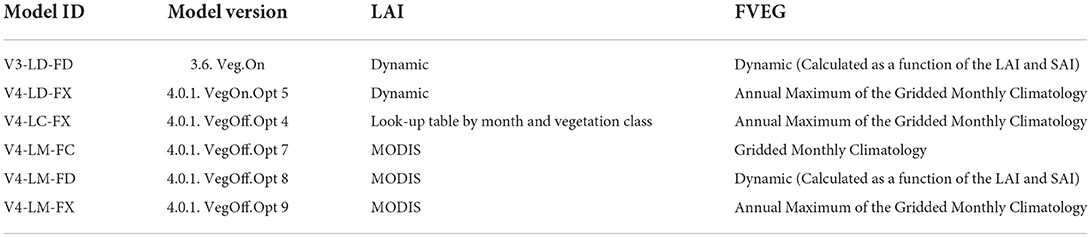
Table 1. Description of each Noah-MP configuration option used in this study.
The gridded runoff and baseflow from the Noah-MP model were used in conjunction with a hydrologic routing model that mimics the movement of water through the natural stream channels, based on topography and stream channel characteristics. The routing model utilized the 30 arcsec (~1 km) HydroSHEDS topography dataset (Lehner et al., 2008) and a slope-adjusted velocity parameterization based on the work of Gong et al. (2009). Although this routing algorithm only solves for continuity and not momentum, it provides a computationally efficient method that has been utilized in several hydrologic monitoring and forecasting applications (Sheffield et al., 2013; Yuan et al., 2015).
Two important vegetation characteristics within the Noah-MP model are LAI and the greenness FVEG. Within the model, the greenness fraction represents the percentage of the grid that is covered with vegetation and the LAI represents the vertical thickness of the vegetation, and therefore, the total evaporative surface area. The Noah-MP model simulations differ in the way LAI and FVEG are calculated in the model. The Noah-MP model can be run with the dynamic vegetation either off or on. When it is turned on, the LAI, stem area index (SAI), and FVEG are predicted from the vegetation model of Dickinson et al. (1998) with default parameters, and the Ball-Berry (Ball et al., 1987) model is used for stomatal resistance.
To help organize and analyze the different model versions, a three-part naming convention is used (Vx-Lx-Fx) where the first part denotes the model version (Vx), the second part denotes the LAI source (Lx), and the third part denotes the FVEG source (Fx). The Noah-MP model version in this analysis will be version 3.6 (V3) or version 4.0.1 (V4). There are three options for the LAI source which include: dynamically calculated by the model (LD), from a Noah-MP look-up table climatology by month and by vegetation class (LC), and LAI from 8-day MODIS measurements interpolated into a daily input variable (LM). There are also three options for FVEG which include: dynamically calculated by the model (FD), the monthly climatology input gridded dataset (FC), and the annual maximum of the gridded monthly climatology at each grid point (FX). Using this convention, the V3-LD-FD model run uses version 3.6 with LAI and FVEG from a dynamic simulation of carbon uptake and partitioning. A summary of the six different Noah-MP model versions is given in Table 1. In these runs, V3-LD-FD and V4-LD-FX both use the dynamic vegetation to compute LAI and SAI; however, V4-LD-FX does not calculate FVEG but instead uses the annual maximum FVEG from the monthly climatological gridded data. The V4-LC-FX does not use dynamic vegetation; instead, the LAI is based on the monthly look-up table values, and the FVEG is based on the annual maximum FVEG from the monthly climatological gridded data. It should be noted that the values of monthly climatology FVEG and the look-up table LAI prescribed for each land use type vary among months but have no interannual variability. Versions V4-LM-FC, V4-LM-FD, and V4-LM-FX use LAI from MODIS real-time data. The difference among these models lies in FVEG configurations. This combination of model simulations will facilitate the assessment of the representation of vegetation in the Noah-MP model and its impact on surface fluxes and streamflow in the model. The simplified representation of groundwater and runoff option (SIMGM) was used in all configurations.
Methods
Simulation results are compared with EC flux measurements of water and energy, time series of soil moisture, and MODIS LAI observations. While ground observations from flux towers (e.g., Ameriflux network) are preferable to satellite-based observations, the absence of field measurements of LAI necessitates a comparison with satellite retrievals of LAI. We aggregated LE, GPP, NEE, and LAI data sets to monthly composites averaged over the entire study period for both model and observations. By focusing on the effects of vegetation dynamics on the near-surface flux exchanges, we highlighted the growing season period (from April to September) at both sites. It should be noted that the MODIS LAI input data was upscaled from the finer resolution of the data product (500 m) up to the model resolution (1/8°grid or ~12.5 km) via averaging. Model comparisons with the EC data are made by comparing the model grid cell that covers the tower locations as shown in Figure 1. The model performance for LE and GPP fluxes was evaluated and summarized in Taylor diagrams using the Pearson correlation coefficient (r), normalized standard deviations (sd), and root-mean-square error (RMSE).
To quantitatively assess the simulated streamflow with the USGS gauge observations and model outputs for LE with MODIS, the Kling-Gupta efficiency (KGE) was used as a dimensionless performance metric. It is defined as:
where r is the Pearson correlation coefficient, μ and σ are the mean and standard deviation of the simulated (s) and observed (o) values, respectively. The KGE can range between –∞ and 1 with the value equal to 1 indicating a perfect match between model simulations and observations. The advantage of the KGE is that it accounts for correlation, variability, and bias of simulated time series and equally weights each metric. Compared to traditional fit metrics, such as RMSE or Nash-Sutcliffe Efficiency (NSE; Nash and Sutcliffe, 1970), the KGE provides more insight into the model skill and the ability to evaluate different components of overall error (Gupta et al., 2009; Fowler et al., 2018; Ghimire et al., 2020). A meaningful benchmark for the KGE is one in which the observed mean is used as a predictor and yields a KGE score of 1 – √2 ≈ −0.41 (Knoben et al., 2019). Therefore, in evaluating the streamflow and LE, the benchmark of −0.41 is considered a lower limit (i.e., minimum KGE threshold), and values below that are not directly quantified but considered poor model simulations. To eliminate water resource management effects on the results, basins with storage greater than 10% of the mean annual streamflow from the USGS were not considered in the analysis.
To identify drought events across the state of Kansas, two drought events, 2012 and 2018 were selected based on the data archive from the U.S. Drought Monitor (USDM). The event in 2012 was the most severe and widespread drought in Kansas since 1988 in terms of both duration and spatial coverage (Anandhi, 2016), while the 2018 drought was milder and less extensive (Chen et al., 2020). In the model, the percentile of the top 1-meter SM (root zone) is used as an indicator of drought-induced water stress. The percentile is calculated as a 30-day moving average for each day of the year using the top 1-m SM with the percentile distribution based on a 14-day moving window centered on the target day over the 11-year simulation period. The USDM was compared to simulated SM based on the following percentiles: greater than 31 is considered no drought, between 21 and 30 is considered abnormally dry (D0), 11–20 is considered moderate drought (D1), 6–10 is considered severe drought (D2), 3–5 is considered extreme drought (D3), and 0–2 is considered exceptional drought (D4) as in USDM drought severity classification (Hayes et al., 2012). The model representation of drought is then compared with the weekly USDM maps.
Results
Overall model performance
Site level
The differences in the simulated land surface water and carbon fluxes, between the sites, are compared against the tower observations to evaluate the performance of the different model configurations. Comparisons among year-round daily LE and GPP from different model versions at both KON and KFS sites are summarized in the Taylor diagrams where the EC data are used as a reference (Figure 2). Overall, there is no significant difference among models in capturing LE at both sites. At KON, LE output from all models falls over the normalized standard deviation of 1 which indicates that all models could regenerate variability in the data compared to the measurements. Whereas at KFS, the simulated LE from all models have more variability than the measurements (since they extended beyond the solid line with sd = 1). GPP products from V3-LD-FD and V4-LD-FX are close to each other but V4-LD-FX is slightly closer to the observed point. The dominant factor contributing to biases in modeled LE and GPP is the choice of LAI and FVEG (Figure 2). Both MODIS LE and GPP were calculated using observed or gap-filled climatological LAI in MODIS collection 6 to maximize the available reliable data. Therefore, potentially poor-quality LAI could influence LE and GPP and may dampen their inter-annual variability. The correlation coefficients of LE and GPP at the KON site range from 0.75 to 0.80 and from 0.60 to 0.70 for the simulations, while LE and GPP correlation coefficients at the KFS site are slightly lower, 0.70–0.75 and 0.45–0.58, respectively (Figure 2). At each site, RMSE values for LE and GPP (presented with gray arcs in Figure 2) are similar. But compared to the KON site, RMSE increased from 0.75 to about 1 at the KFS site, which reveals a higher degree of agreement between the simulated LE and GPP from different model versions and field measurements at the KON site. One of the reasons for the differences in the two locations is that the dominant land cover type at the KON grid cell in the model is consistent with dryland cropland and pasture as compared to the KFS grid cell which is mainly characterized as cropland/grassland mosaic.
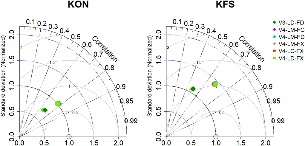
Figure 2. Taylor diagrams for comparing model performance: (circles) latent heat (LE) and (diamonds) gross primary production (GPP) from both KON and KFS sites. The radial distance from the origin is the normalized standard deviation and the correlation coefficient is displayed as the azimuthal position. All statistics are calculated on a daily time scale from 2008 to 2018 and colors represent different models consistent with the color codes.
Seasonal fluxes
To take a wider view of the role of dynamic phenology and the ability of the models to simulate the water and carbon cycle, 11-year average seasonal cycles of climatological fluxes are summarized in Figure 3, 4. It should be noted that the results of all model configurations, using MODIS LAI as input are qualitatively very close in all output variables at seasonal cycles at the two study sites. Therefore, LAI and FVEG model outputs nearly overlap each other (purple, cyan, and tan lines). At the KON site, all model configurations overestimate the climatological LE during the early growing season (Mar-Apr). However, the difference between EC measurements and all model simulations decreases substantially in the middle of the growing season (June) when the leaves are fully developed, and fluxes are large and continue until the end of the year. Accordingly, at the KFS site, all configurations overestimated the LE during the early growing season with the largest positive bias in June (Figure 3). Model performance is reflected in 11-year averaged KGE scores between simulated and MODIS LE for different model versions at each site. At KON and KFS sites, the V4-LM-FX model provides a better fit (with KGE = 0.345 and KGE = 0.737, respectively) between simulated and measured LE. At KFS, all model versions overestimate LE in comparison to EC observations but again V4-LM-FC and V4-LD-FX provide a better match with more accuracy leading to higher KGE values. Although the difference between simulated LE from all versions at both sites increases rapidly at the beginning of the growing season, this deviation becomes smaller particularly at the KON site during the later growth stages. The peak value of the modeled LE at both sites happens in June which is consistent with the measurements. Observed LE values from the early vegetative stage (April to July) represent sharp (at KON) and gradual (at KFS) rise and moderate decline during the late season from August to September at both sites. Simulated sensible heat fluxes (H) from all model versions were less at both sites for the first 6 months of the year compared to the EC measurements. These differences diminished from the middle of the growing season until the end of the year and the simulated H pattern became more consistent with the observations, especially at the KFS site. The result of two versions of the model (i.e., V3-LD-FD and V4-LD-FX) compared with MODIS and EC measurements of GPP are also presented. Both versions of the model were able to reproduce the trend of carbon uptake compared to the flux measurements. Except for 3 months in the middle of the growing season (June–August) at the KON site and 1 month (August) at the KFS site, both models overestimate GPP. Like LE, peak simulated GPP happens in June which is almost 50% larger at the KON than the KFS site (Figure 3).

Figure 3. Seasonal climatology of simulated LE, leaf area index (LAI), fractional vegetated area (FVEG), and GPP from different Noah-MP configurations vs. MODIS and EC measurements during the 11-year study period for KON and KFS sites. Gray-shaded areas denote the growing season.
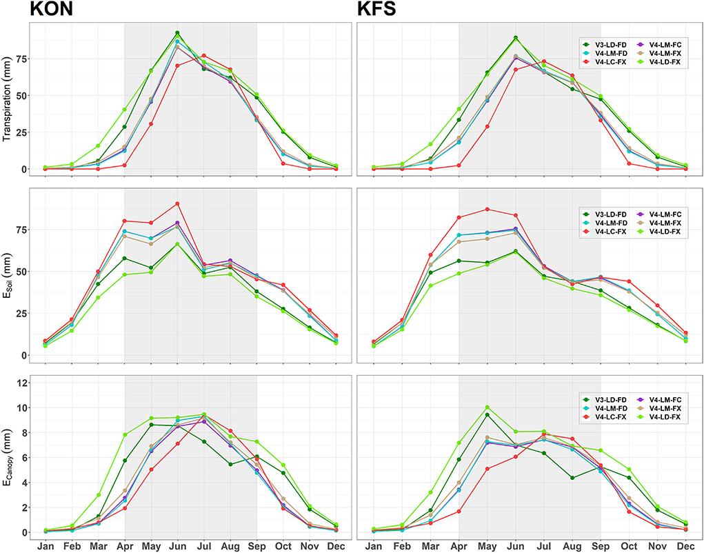
Figure 4. Seasonal climatology of simulated Transpiration, Ecanopy, and Esoil from different Noah-MP configurations vs. MODIS and EC measurements during the 11-year study period for KON and KFS sites. Gray-shaded areas denote the growing season.
It should be noted that upscaling finer grid cells to coarser resolution resulted in a difference between the MODIS LAI value for a single tower pixel and MODIS measurements used in the model (divergence between all the MODIS-derived LAI model versions and blue dots, Figure 3). In addition, the difference among green vegetation fraction of versions using maximum climatology FVEG in winter months (January, February, and December) reflects the canopy height variation relative to the snow depth. When snow cover is higher than the vegetation height, the FVEG will drop below its maximum value in the model.
One of the main takeaways from Figure 3 is that there is little deviation in the LE flux across model configurations despite the fact that the models vary substantially in their representation of LAI. To explore this in more detail, the components of LE including transpiration, soil evaporation (Esoil), and canopy evaporation (Ecanopy) are shown in Figure 4. It is important to note that the units in Figure 4 are mm (evaporation) and not w/m2 (latent heat flux) as in Figure 3. Despite the insensitivity of LE to the impact of vegetative properties at both sites, there is a distinct difference among individual components of LE for each model configuration. Specifically, transpiration and canopy evaporation vary directly with the LAI and models that show higher initial LAI show a larger transpiration and canopy evaporation. It should be noted that canopy evaporation is relatively small (about 10 times smaller) as compared to the other components. Even though there is a high connection between model LAI and transpiration and canopy evaporation, this is offset by much lower soil evaporation. This tradeoff between soil transpiration, canopy evaporation, and soil evaporation results in little difference between the total LE in all model simulations and indicates that models are primarily operating in an energy-controlled regime.
Simulated fluxes during drought events
Figure 5 presents the diurnal time-series of measured and NLDAS-2 forcing precipitation, SM percentile, simulated transpiration, and simulated vs. measured LE throughout two selected drought years (2012 and 2018). The simulation results of both sites show a nearly similar pattern; therefore, only the results of KON will be discussed. For all model versions, LE converges together when there is a precipitation event according to the NLDAS-2 atmospheric forcing data which indicates that all versions have a similar behavior when the soil is well watered. The large differences between modeled and measured LE values generally occur during inconsistencies between daily gauge measurements and NLDAS-2 rainfall forcing data. Top 1-m SM percentiles from all model versions slightly diverge from each other during the late winter and early spring but they show a very similar behavior throughout the growing season in both years. Despite the subtle variation, among SM percentiles from all model versions in the rest of 2018, there is a noticeable contrast among SM percentiles throughout the fall and winter of 2012. The behavior and magnitude of transpiration are almost identical in all the MODIS-LAI-based models and the pattern is very similar to the model versions with dynamic vegetation (e.g., V3-LD-FD and V4-LD-FX). However, there is a distinct separation between V3-LD-FD and V4-LD-FX, especially during the summer and early fall. Version with prescribed LAI (V4-LC-FX) failed to capture seasonal variability of LAI and FVEG and express a different transpiration pattern compared to the other version.
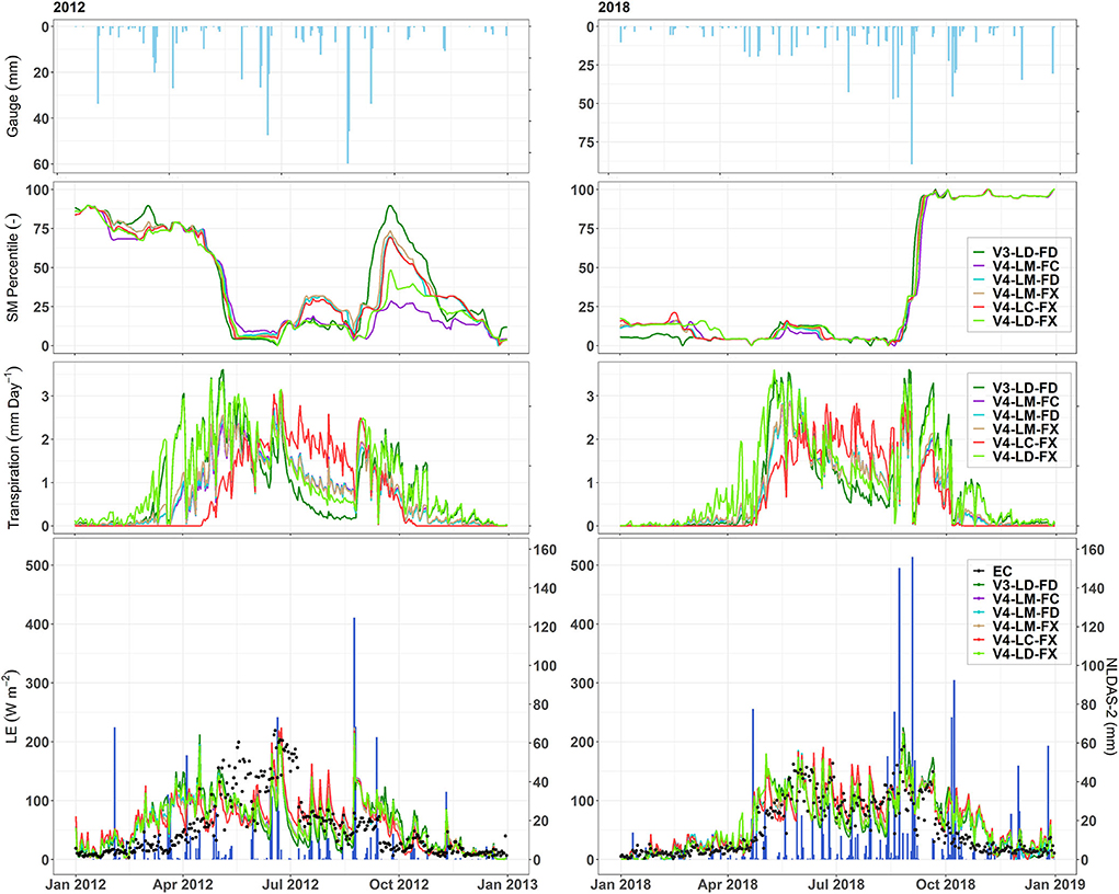
Figure 5. Precipitation, top 1-m soil moisture percentile, transpiration, and LE at the KON site for two selected drought years (2012, left; and 2018, right). (Top panels) Gauge precipitation measurements at the site; (Second row) top 1-m soil moisture percentile; (Third row) Transpiration; (Bottom panels) Comparison of average daily simulated LE from all different Noah MP configurations (various colored lines) vs. EC measurements (black dots) and NLDAS-2 precipitation forcing (blue bars).
As shown in Figure 6, both V3-LD-FD and V4-LD-FX capture the general trend of LAI during the drought years. Except for a few months at the beginning of the growing season, V4-LD-FX overestimates LAI during both events. However, V3-LD-FD underestimates LAI in the middle and late growing season. Both leaf onset and LAI ramp-up occur much faster compared to MODIS-LAI measurements in both V3-LD-FD and V4-LD-FX models in 2012 and V4-LD-FX in 2018 which leads to higher LE during the growing season length. Measured and forcing precipitation were generally close to each other from January to April in both years. From the early growing season, NLDAS-2 starts to produce more precipitation, particularly in 2018 which results in a higher cumulative precipitation difference between the forcing and gauge measurements (Figure 6, third panel). There is a good agreement between all model versions simulated and in-situ measurements of SM in the top 10 cm, but this agreement fades after June during the 2018 event. The overestimation of soil moisture depletion during drying phases was greater in V4-LC-FX than in other versions. This version assumes fixed vegetation conditions for each year which leads to relatively higher ET loss estimates in both dry years, and a sharper decline of soil moisture at deeper layers (30–100 cm), especially during maximum plant development, whereas dynamic LAI phenology in other versions simulates changes in leaf area and reproduces more realistic drought-induced vegetative stress and SM trend.
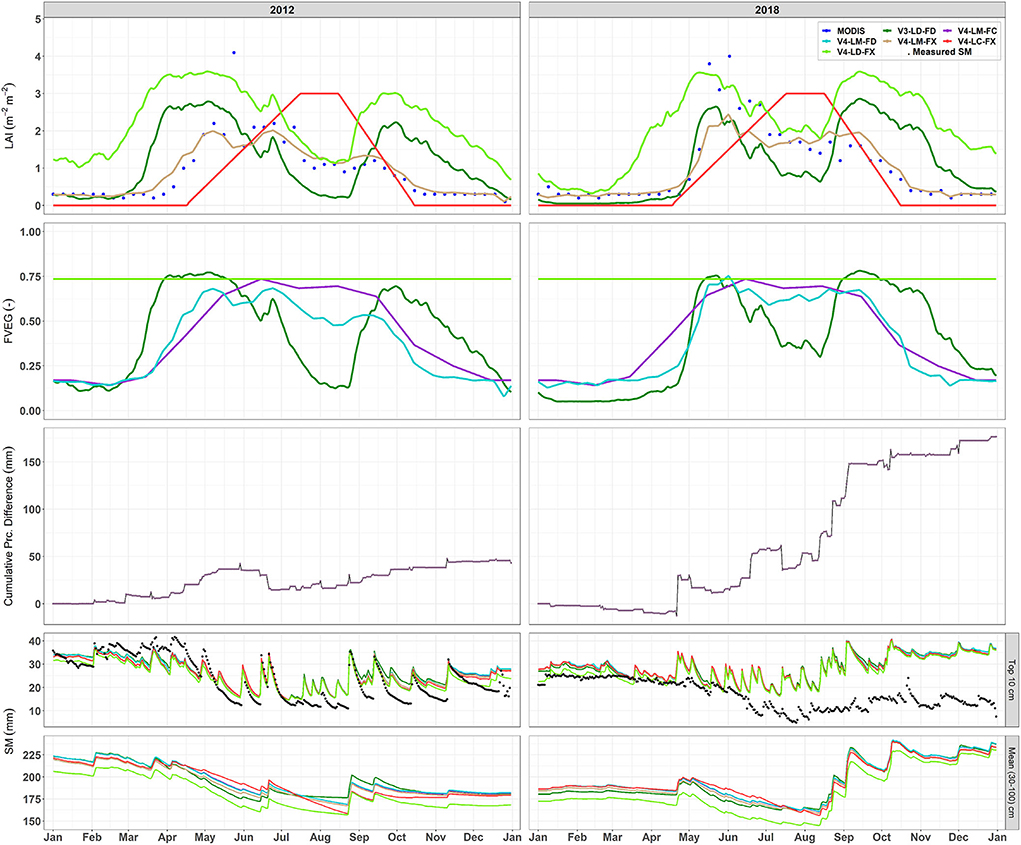
Figure 6. Comparison of average daily simulated LAI from all different Noah-MP configurations vs. MODIS measurements (top panel), simulated FVEG (second panel), and simulated soil moisture for the top layer (10 cm) compared to the field measurements (black dots) and average soil moisture for the three bottom soil depths (30, 60, and 100 cm) (bottom panels) throughout the selected drought years (i.e., 2012 and 2018) at the KON site.
Domain level
Latent heat flux
Figure 7 shows the spatial distribution of the 11-year domain-averaged mean seasonal KGE values between simulated and MODIS LE for the different model versions. The overall spatial patterns are consistent for all model versions with the highest values in the eastern part of the state and low values in the western portion of the state. A comparison of MODIS and modeled climatology indicated that all model versions overestimate LE over the entire state particularly in the central and western parts of the state (see Supplementary Figure S1). Analyzing the components of KGE reveals that except for small areas in the middle and southwest of the state, the overall correlation component is very close to unity over the entire region (Supplementary Figure S2). This reflects the ability of the model to reproduce the timing and shape of the seasonal cycle as measured with no clear tendency for systematic errors (Supplementary Figure S3). The areas with a higher ratio of the simulated and observed standard deviation corresponded with lower KGE values. In the central and eastern parts of the state, the ratio of the simulated mean and observed mean (bias ratio) for the LE flux is closer to 1 (Supplementary Figure S4). This spatial pattern is more evident in MODIS-retrieved LAI versions (i.e., V4-LM-FC, V4-LM-FD, and V4-LM-FX). The large variability in LE from all the model versions other than MODIS in the western portion of the state indicates that the limitation of the model is mainly governed by the overestimation of variability.
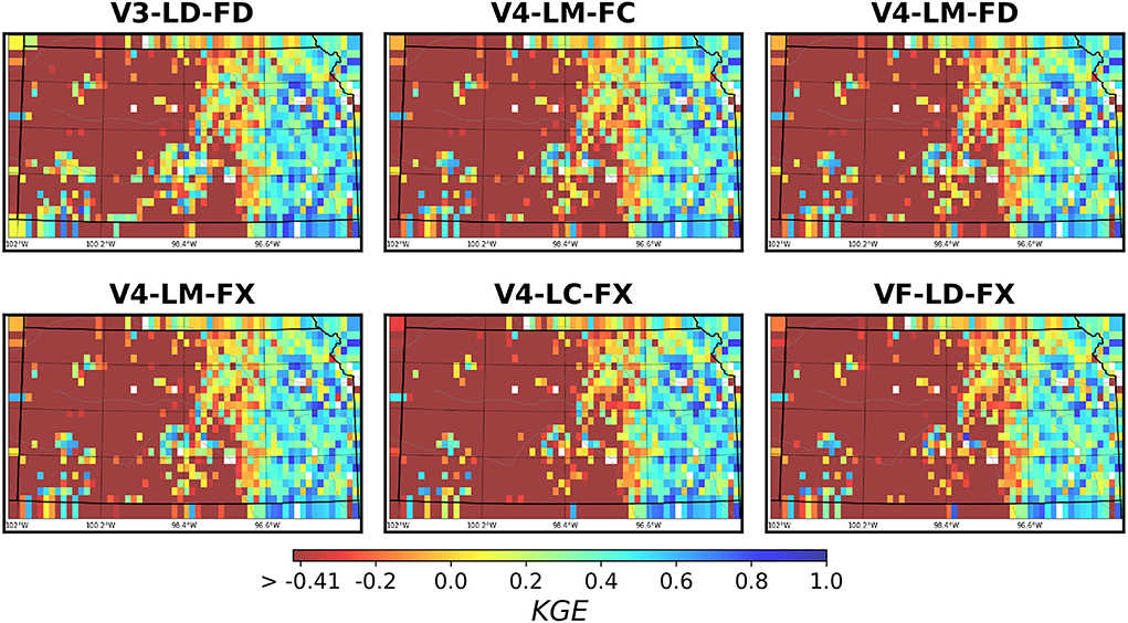
Figure 7. Spatial distribution of seasonally averaged Kling-Gupta efficiency (KGE) of LE flux (W m–2) between each Noah-MP configuration and MODIS. For the three assessment criteria, a value of 1 indicates a perfect agreement between MODIS and the simulations. The minimum threshold is set to −0.41 for any KGE values ≤ −0.41.
To further evaluate the performance of each model, Figure 8 shows the 11-year climatological averaged LE of three selected grid cells. The three grid cells were selected based on the average KGE values across all model runs. The difference among simulated LE from all versions is not very noticeable at the selected grid cells with minimum and maximum KGE values although this divergence becomes more pronounced at the location with a minimum KGE value. The peak of the LE at the grid cell with the highest KGE value happens in June which is consistent with the MODIS measurements (Figure 8A). At the selected grid with a minimum KGE value, the MODIS LE is very low and does not vary over the year, but all model versions demonstrate a similar but higher LE (Figure 8B). The primary land cover type at this grid cell is comprised of sedimentary rocks. This issue could be attributed to the MODIS inaccuracy and model limitations in land cover type identification. The low and quite constant MODIS LE values could reflect the absence of water in this unvegetated rocky area. There is a distinct separation among model versions with different LAI and FVEG options at the grid cell with the minimum threshold KGE value which reflects the sensitivity of heterogeneous land-use and spatial locations to LAI and FVEG inputs (Figure 8C). In addition, the grid cell with minimum threshold KGE value of LE from MODIS is shifted to an earlier time (between May and June). Interestingly, LE products from MODIS never dipped below 15 (Wm−2) even in the wintertime compared to much lower EC measured values (≈5 Wm−2), which reflect the limitation of the MODIS LE data (Miranda et al., 2017).
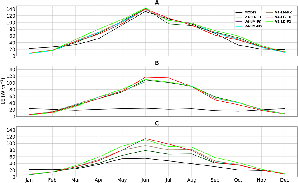
Figure 8. Climatological LE from all different Noah-MP configurations vs. MODIS across the selected domain for the entire study period (2008–2018) for (A) grid cell with the highest KGE value (0.90) located in the western part of the state and the dominant land cover type is classified as grassland, (B) grid cell with minimum KGE threshold (−11.87) located in the eastern part of the state and the dominant land cover type is classified as cropland/grassland mosaic, (C) grid cell with minimum threshold KGE value (−0.42) located in the south-central region of the state and the dominant land cover type is classified as grassland. Here, colors represent different models consistent with the color codes.
Monthly streamflow
To further explore the impact of vegetative dynamics on surface fluxes and the water balance, we evaluated the model's performance for simulating the annual streamflow at 31 basins across the study domain. The median KGE values of the annual average streamflow for all model versions are given in Figure 9. The KGE scores vary among the different models and the study basins. Some gauges consistently perform better or worse than the others in all the models (e.g., the gauges denoted with letters a, b, and c in Figure 9) but most of the gauges do not demonstrate a consistent KGE score across the model configurations. As shown in Figure 9 (lower right), box plots compare the KGE statistics across the model configurations and indicate that the configurations that use measured MODIS-LAI (LM) result in slightly higher KGE values as compared to other configurations. However, there is no significant difference in the model performance among the six configurations, in terms of KGE for the simulated annual streamflow with all versions reflecting the same spatial variations in streamflow across the domain. Although not shown, the majority of basins have a correlation coefficient (r) closer to the ideal value of unity and there was no basin with a negative correlation. The bias ratio between average values for modeled (μs) and measured (μo) discharge and variability component (σs/σo) is less than one for most of the gauges. This represents an underestimation of discharge with lower variability in simulations. The notable underprediction in the streamflow could be the result of an overestimation of evaporation (Figure 3) or a simplified representation of groundwater dynamics in Noah-MP which represents recharge and discharge processes in an unconfined aquifer.
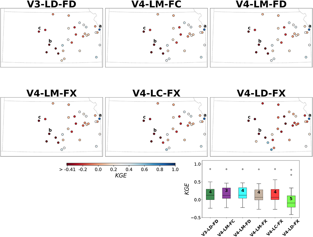
Figure 9. Map of streamflow prediction performance using KGE for 31 selected basins across the model domain, and boxplots of each model configuration with the range from −0.41 to 1. The numbers on the boxplots represent the total number of the gauges below the minimum KGE benchmark value (−0.41). Locations of USGS gauges with maximum (a), minimum (b), and minimum threshold (c) average KGE in this figure are marked on the map.
To further illustrate the streamflow behavior of each model configuration, the mean monthly time series of the simulated streamflow for selected gauges with the highest, lowest, and minimum KGE values are shown in Figure 10. Overall, there was a good agreement between all model version simulations and USGS measurements at the mean monthly time-step for the selected gauge with the highest KGE value (Indian Creek, Overland Park, KS). This gauge is in the northeast part of the state, suggesting good model performances over the subhumid to humid regions of Kansas (Figure 10A). Other gauges with minimum mean KGE value (Rattlesnake Creek near Zenith, KS), and minimum threshold KGE value (Big Creek near Hays, KS) are in the central part of Kansas (gauge locations indicated in Figure 9). At Rattlesnake Creek, all model versions overestimate the monthly averaged runoff regime (Figure 10B). At Big Creek, the simulated runoff followed the trend of the USGS observations reasonably well until 2016 but after that, the simulated streamflow exhibits considerable underestimation of peak low magnitudes (Figure 10C). This could reflect a significant difference between climatic characteristics in the eastern vs. western parts of Kansas. Generally, the western part of the state is characterized by a semiarid climate with hot, dry summer and cold, windy winter and the eastern part tends to be considerably more humid, with sultry summer and cold winter months. This west-east climatic contrast impacts the generation of surface runoff and evaporation which is closely related to rainfall intensity. In addition to spatial patterns in precipitation gradient, in the west and central areas of Kansas, excessive groundwater pumping may lower the water table below the stream-water surface, causing the stream to lose water to the underlying aquifer and decrease the groundwater seepage to the stream. In addition, catchment size and land use characteristics may also affect the runoff retention time. Hydrographs indicate that all the model versions tend to consistently underestimate the peak streamflow in the west and central part of Kansas.
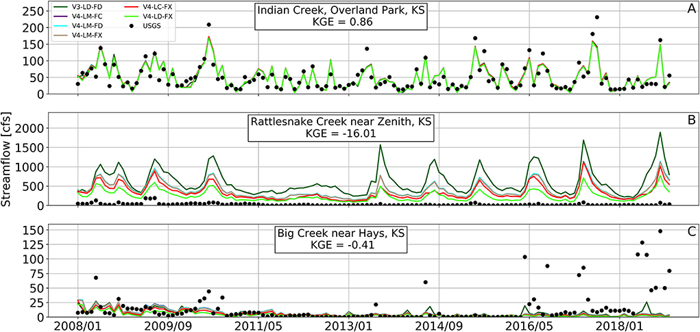
Figure 10. Comparison of monthly simulated streamflow time series with USGS gauge measurements for selected gauges with (A) maximum average KGE (Indian Creek, Overland Park, KS), (B) minimum threshold KGE, (Rattlesnake Creek near Zenith, KS), and (C) minimum average KGE value (Big Creek near Hays, KS).
Model performance evaluation during drought
To investigate the impact of vegetation representation in simulating rapidly emerging severe drought conditions, the simulated top 1-m SM percentile from different model versions over the state of Kansas were compared with USDM drought categories for two selected drought events in 2012 and 2018 (Figure 11). It is necessary to note that some disagreements between the model SM percentiles and USDM are expected since the USDM drought is based on many factors like county-level information on drought, expert opinion of the current impact of the drought on a region, precipitation, streamflow, reservoir levels, snowpack, and groundwater (Sehgal, 2019). Furthermore, the model SM percentiles were calculated using only the 11-year simulation period. Despite these differences, the general agreement is expected, and the USDM can still provide a good comparison to assess the ability of the model to detect drought. In August 2012, exceptional drought (D4 category) covered most of the west and portions of the east part of the state. In August 2018, only some areas in northeast Kansas were affected by the D4 category drought. It can be observed that the top 1-m SM percentile maps from all model configurations in 2012 show much lower drought conditions over the entire state, while USDM indicates exceptional drought over much of Kansas. But both V3-LD-FD and V4-LD-FX versions present a closer spatial resemblance between the model and the USDM map. This is interesting since, despite slight differences among all the 4.0.1 versions, they could replicate the majority of the drought-affected areas in 2018 events. Underestimation of drought magnitude in the large pocket in the central and west part of Kansas during the 2012 event is likely associated with the ability of the model to imitate rapid developing droughts as in 2012. Overall, the behavior of the gridded SM percentile is reasonably consistent with the drought categories on USDM maps in 2018 but there are some differences in case of severe drought areas.

Figure 11. The US Drought Monitor (USDM) and the modeled soil moisture percentile for the top-1 meter of the soil over the state of Kansas on 21 August 2012, and 14 August 2018. Colors indicate drought categories defined by the USDM, from abnormally dry (yellow) to exceptional drought (dark red).
Sources of uncertainties
Overestimation of evaporation (LE) fluxes in the model could be ascribed to uncertainties in the MODIS LAI data and model biases in soil moisture, groundwater storage, or representation of vegetation within the model. In theory, large negative or positive biases in the model-predicted storage are most likely mitigated by overestimation (underestimation) of both outgoing fluxes (i.e., runoff and evaporation) to close water balance in long-term averages (Lin et al., 2018). To understand the possible tendencies in long-term water budget on how changes in one component affect the estimation of the other mutually dependent hydrologic processes, we used a simple water balance equation:
where P is precipitation, E is evaporation, and Q is runoff. In this equation, all variables are expressed as an 11-year average and change in storage is considered negligible under the assumption that there is no trend in storage change and that year-to-year variations cancel each other out over a long period. Since there was no statistically significant difference among the other version outcomes, the result of V4-LD-FX is presented here (Figures 12, 13). In Figure 12, each dot represents one of the 31 selected drainage areas of the USGS gauges within the study domain. The color scheme presents 11-year average NLDAS-2 annual precipitation. The estimated average evaporation from all models and water balance is expected to show a very close relationship, but it is noted that there are more dispersions around the line with a slope of unity compared to the model vs. water balance evaporation (Figure 12). This deviation pattern is even more evident for basins with drier conditions (average annual precipitation <900 mm), especially in MODIS vs. water balance evaporation comparison (Figure 12B). It is apparent that both the model and water budget overestimate evaporation in comparison to the MODIS data, but the model exhibits the highest level of prediction accuracy (R2 = 0.80). These results are consistent with the findings reported by Brunsell et al. (2021). Among all versions, the V3-LD-FD presents the lowest agreement between Noah-MP and water balance vs. MODIS evaporation (R2 = 0.73 and R2 = 0.48, respectively).
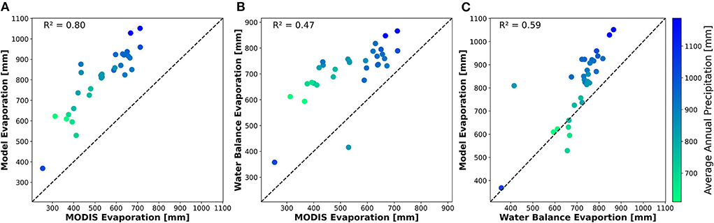
Figure 12. Scatter plots of V4-LD-FX version (A) Noah-MP evaporation vs. MODIS, (B) estimated evaporation from water budget vs. MODIS, and (C) estimated evaporation from water budget vs. model for 31 selected basins using an 11-year averaged. The color bar indicates the 11-year average precipitation (mm) over selected basins within the domain from higher (blue) to lower (green) values.

Figure 13. Comparison of V4-LD-FX version vs. USGS gauge streamflow measurements for 31 selected basins. The color bar presents the difference in simulated and water budget evaporation during the 11-year average.
Figure 13 illustrates the relationship between USGS gauge measurements with averaged runoff estimations of V4-LD-FX for the 31 selected drainage areas and the color bar indicates the difference between water balance and model streamflow. We observed that the streamflow is reasonable by model simulations (R2 = 0.49). However, simulated streamflow is underestimated compared to USGS measurements. The results of the surface runoff analysis suggest that the overestimation of evaporation is characterized by the underestimation of peak-flow magnitudes which indicates more water should be retained in the soil layers instead of evaporating into the atmosphere. This might also be attributed to a poor estimation of the model parameters or due to an interaction of the model parameters that had a significant effect on the dominating processes in that flow range. Here again, we noticed that V3-LD-FD exhibits less agreement between Noah-MP and USGS gauge measurements (R2 = 0.30) among all models.
The extreme point on the lower-left corner of the scatter plots (Figures 12A–C) does not follow the same pattern on the precipitation gradient. This point represents a basin on the northeastern border of the state that is heavily urbanized. Despite a relatively high 11-year average precipitation, the rate of the LE is very low. Significant low evaporation at this basin is a compound result of the reduction in LAI and diminishing of transpiration from vegetation and evaporation lost from canopy interception which promotes wetter soil conditions and greater surface runoff. This is also noticeable in the close value of the averaged runoff of all models to the USGS measurement (extreme upper-right point in Figure 13). In addition, impervious land covers in urban areas have a pronounced effect on bare soil evaporation.
Figure 14 compares the ability of the model in simulating the LE as a KGE score vs. the 11-year annual average of NLDAS-2 meteorological forcing [i.e., air temperature, precipitation, specific humidity, wind speed, downward shortwave (SW), and longwave (LW) radiation] for the dominant USGS land cover categories across the model domain. Surface pressure was excluded from this analysis due to its undetectable impact on the relationship between LE performance and landcover type. Due to a similar pattern among all model version outcomes, the result of V4-LD-FX is presented here. Cropland/grassland mosaic and grassland land cover types exhibit lower KGE value in hot and dry conditions (low precipitation and humidity and high shortwave radiation). The impact of wind speed and air temperature on the specific land cover type was not very clear. Only dryland cropland and pasture (DCP) present relatively lower KGE in response to higher air temperature. Based on the USGS land-cover category, much of the western part of the state is classified as cropland/grassland mosaic and grassland in the model. Irrigated croplands impact the thermodynamics of the sensible and latent heat fluxes. Moreover, with a high level of soil water content, the LE becomes independent of the soil moisture in energy limited ET regime. Evaporation links the water balance to the surface energy balance with the heterogeneity of the landscape being accounted for by land cover type in the model. Therefore, an investigation of land cover–precipitation feedback and its impact on model performance is suggested for future studies.

Figure 14. The variation of the KGE between the model and MODIS LE flux with respect to the dominant land cover and the 11-year mean annual NLDAS-2 forcing components including precipitation, air temperature, specific humidity, downward shortwave (SW) and longwave (LW) radiation, and wind speed.
Discussion
The dynamic vegetation scheme in the land surface model significantly influences the water and carbon budgets of terrestrial hydrological modeling. In this study, we investigated the impact of including and excluding Noah-MP dynamic vegetation function on key water and carbon budget terms by comparing six different model configurations against field measurements. The difference in each version is related to the calculation of LAI and FVEG. The simulation results reveal the difference between dynamic leaf model calculation of LAI estimates (V3-LD-FD and V4-LD-FX) and LAI from MODIS real-time data (V4-LM-FC, V4-LM-FD, V4-LM-FX) at the point-scale for two selected study locations and were able to reasonably capture the temporal variability of the LE component (i.e., transpiration, Esoil, and Ecanopy) and sensible heat flux. The Noah-MP model requires the conservation of the partitioning of total net radiation (Rn) energy that reaches the land into sensible and LE and soil heat fluxes (Pitman, 2003; Niu et al., 2011; Best et al., 2015). As a result, portioning of Rn could impact the ability of the model for predicting both sensible and latent heat fluxes. With enough soil moisture, the Noah-MP uses the remaining energy to evaporate water from the soil into the atmosphere resulting in the unchanged magnitude of the total LE. The result from performance matrices in Figure 14 also indicates that a lower KGE score for the simulated LE is connected to limited incoming shortwave radiation over dominant domain landcover types. At the site level, V3-LD-FD and V4-LD-FX simulations captured the observed seasonal trend of GPP, but they underestimated the GPP during peak growing seasons. The underestimation of LAI during the growing season is attributed to less carbon allocation to leaves and lower GPP during the growing season (Figure 3). This reflects the greater photosynthetic capacity of dominant C4 grassland with a more rapid accumulation of green leaf area than C3 plants in the model (Figure 3).
In addition to LAI and FVEG, in all model versions, the stomata are controlled mainly by average soil water availability (or β factor), leaf maximum carboxylation rate (Vcmax) and maximum rate of carboxylation by the enzyme, Rubisco (Vcmax25) which are treated as vegetation type-dependent constants. The only recognition of hydrodynamic properties of plants in Noah-MP is the rooting depth. But rooting depth only indicates which soil layers need to be incorporated in a single average number of soil moisture that ends up controlling the stomata. However, Wang et al. (2018) showed that replacing static root profile with dynamic root optimization in the default Noah-MP resulted in more realistic root response to ET between wet and dry seasons. Plant water use efficiency (WUE) remains a major challenge for simulations of diurnal dynamics of transpiration (Matheny et al., 2014). Root zone soil moisture also has a direct impact on baseflow and streamflow simulations.
A rapid shift in vegetation emergence than the actual plant coverage implies that current Noah-MP versions are generally missing in important processes, such as the negative lagged effect associated with warmer springs which consequently lead to the buildup of water stress (Wolf et al., 2016; Buermann et al., 2018; O'Sullivan et al., 2020). Again, mainly due to the spatial scale difference between satellite observations and model grids, there is a discrepancy between MODIS observation at the flux tower and simulated LAI in all the MODIS-LAI-based model versions.
Implementation of prescribed LAI/FEVG with the same vegetation values every year can generate abnormally high ET during dry conditions and exacerbate soil moisture deficits. To address this issue, enormous efforts have been made to introduce dynamic growth simulations into Noah-MP over the last decade. Liu et al. (2016) introduced dynamic growth simulations and field management for two summer crops (corn and soybean) into Noah-MP (Noah-MP-Crop). Additionally, Ingwersen et al. (2018) extended Noah-MP by a dynamic crop growth component (Gecros; Xinyou, 2005) for winter wheat and maize. Plants subjected to long-term or severe drought stress cannot reach the same level of transpiration after the cessation of a drought which can cause disagreement between the model and measured LE (Su et al., 2021).
At the domain scale, the inconsistency in evaporation between the models and MODIS in the central and western parts of Kansas shows that all models failed to simulate LE correctly over this region (Figure 7). This could be largely due to the discrepancies between prescribed and real land cover classes. Additionally, this could be attributed to shortcomings in the irrigation routine in Noah-MP, since irrigated croplands in the western part of Kansas enhance ET. One must bear in mind that incorporating an improved land-cover dataset in the model is crucial to properly representing surface processes on both meteorological and climatological scales. In addition, previous studies (Heinsch et al., 2006; Miranda et al., 2017; Pu et al., 2020) have addressed the tendency of MODIS to overestimate LAI which may lead to the miscalculation of vegetation cover fraction and overestimates of evaporation.
Compared to the field measurements, the simulated SM from all model versions in 2018 shows larger disagreement in the middle of the growing season when leaves are fully developed, and the plant is able to transpire water approximately at rates equivalent to the atmospheric demand. This is accompanied by overall higher precipitation forcing in the model compared to 2012. Therefore, precipitation differences in the early summer of 2018 represent a significant source of forcing condition uncertainty and cause a noticeable divergence between modeled and measured SM which remains throughout the year. A rapid shift in the vegetation emergence than the actual plant coverage implies that current Noah-MP versions are generally missing in important processes, such as the negative lagged effect associated with warmer springs which consequently lead to the buildup of water stress (Wolf et al., 2016; Buermann et al., 2018; O'Sullivan et al., 2020). Again, mainly due to the spatial scale difference between satellite observations and model grids, there is a discrepancy between MODIS observation at the flux tower and simulated LAI in all the MODIS-LAI-based model versions.
The overall results show that there is a major impact of rainfall forcing on all model versions. From simulations, it is evident that NLDAS-2 precipitation forcing significantly impacts the simulated LE fluxes of all model versions. The discrepancies in precipitation between NLDAS-2 forcing and gauge measurements exert a great impact on the general performance of the simulated compared to the observed LE and SM. At both sites, there is a clear response trend between the magnitude and timing of daily gauge-based precipitation and measured LE. Investigating the cumulative gauge-measured and NLDAS-2 precipitation of selected drought years indicates that not only is there a difference in terms of timing and magnitude of each event but also the total depth of the annual rainfall. Furthermore, the gradual decline of water content in the topsoil layer results in a dramatic decrease in LE, especially during the drought years. However, the drought had little impact on LE simulation whenever there is sufficient water input from large precipitation events at the beginning of the growing season. The relative insensitivity of the model LAI to the overall LE suggests that the evolution of LSMs has focused more on obtaining correct surface fluxes instead of accurate reproduction of SM products (Entekhabi et al., 2010). We should note that while NLDAS-2 may provide the most realistic retrospective forcing data, aggregating reanalysis, radar data, and rain gauge measurements into a grid, tends to crucially smooth precipitation in space and time (Luo et al., 2003). In North American mesic grasslands, precipitation is a strong driver of C4 grass productivity during the growing season (Brunsell et al., 2014; Wagle et al., 2015), which is reflected in a higher degree of carbon uptake, especially at the KON site.
In particular, this study shows that the difference in land-cover type has the potential to affect couplings between carbon and water fluxes at the land surface and alter land model simulations. It is also important to note that Noah-MP features four vegetation carbon pools (leaf, stem, root, wood), and two soil carbon pools (fast and slow) (Niu et al., 2011; Yang et al., 2011). Hence, updating the surface exchange coefficients and parameters specifically related to the dynamic vegetation components also plays a significant role in the determination of the vegetation impact.
Conclusion
Multiple vegetation physical options available in the Noah-MP LSM were evaluated on the overall skill of their model predictions over various landcover types. This study demonstrates the response of carbon and water fluxes to vegetation components (i.e., LAI and FVEG) based on 11 years of Ameriflux observations, particularly during two major drought events over the midwestern United States. Decomposing LE flux components reveals that the apparent insensitivity of simulated LE to LAI and dynamic vegetation process can be attributed to the tradeoff between soil evaporation and transpiration. The Noah-MP employs a closed energy budget. In the presence of adequate soil moisture, the incoming net radiation limits ET, and both the sites are generally operating in an energy-limited regime. With high surface and root zone soil moisture, water can be extracted from the soil for evaporation and the total amount of ET from each model remains similar which reflects constraints associated with the Noah-MP that could be linked to the forcing. Overestimation of LE resulted in underestimation of runoff, especially over heavily cultivated basins that cover much of the western and central parts of the state.
Although the Noah-MP LE and GPP differ from the observation datasets at the selected sites, it is still considered a satisfactory proxy of water and carbon fluxes in the absence of better estimates like flux tower measurements. Recent work by Kumar et al. (2019) and Mocko et al. (2021) have found that data assimilation of LAI into the dynamic vegetation scheme of Noah-MP improves the simulation of ET and GPP, particularly in the agricultural areas of the United States. LSMs include a myriad of surface processes and vegetation parameters that ideally would be regionally tuned, leading to difficulties in vegetation specification and uncertainties in their outputs, especially under extreme climate conditions like drought. Promising future model enhancements will potentially improve the ability of the model to capture vegetation dynamic behavior, especially under extreme climatic conditions.
Data availability statement
The original contributions presented in the study are included in the article/Supplementary material, further inquiries can be directed to the corresponding author/s.
Author contributions
AH carried out the Noah-MP assimilation runs, analyzed, and wrote the manuscript. JR conceived the study and supervised AH to implement all the research ideas. NB provided the EC data and contributed to the interpretation of the results. DM developed the code to use the MCD15A2H.006 LAI data within the LIS framework for its use within the Noah-MP LSM and provided valuable feedback during the model debugging phase. SM processed the MCD15A2H.006 LAI data into an analysis-ready netCDF-4 format for use within the LIS software framework. SK and KA provided support for data set implementation in Noah-MP LSM. All the authors discussed the results and implications and commented on the manuscript at all stages. All authors contributed to the article and approved the submitted version.
Conflict of interest
DM, SM, and KA were employed by Science Applications International Corporation.
The remaining authors declare that the research was conducted in the absence of any commercial or financial relationships that could be construed as a potential conflict of interest.
Publisher's note
All claims expressed in this article are solely those of the authors and do not necessarily represent those of their affiliated organizations, or those of the publisher, the editors and the reviewers. Any product that may be evaluated in this article, or claim that may be made by its manufacturer, is not guaranteed or endorsed by the publisher.
Supplementary material
The Supplementary Material for this article can be found online at: https://www.frontiersin.org/articles/10.3389/frwa.2022.925852/full#supplementary-material
References
Anandhi, A., and Knapp, M. (2016). How does the drought of 2012 compare to earlier droughts in Kansas, USA. J. Serv. Climatol. 9, 1–19. doi: 10.46275/JoASC.2016.05.001
Arsenault, K. R., Nearing, G. S., Wang, S., Yatheendradas, S., and Peters-Lidard, C. D. (2018). Parameter sensitivity of the Noah-MP land surface model with dynamic vegetation. J. Hydrometeorol. 19, 815–830. doi: 10.1175/jhm-d-17-0205.1
Baldocchi, D., Falge, E., Gu, L., Olson, R., Hollinger, D., Running, S., et al. (2001). FLUXNET: a new tool to study the temporal and spatial variability of ecosystem-scale carbon dioxide, water vapor, and energy flux densities. Bull. Am. Meteorol. Soc. 82, 2415–2434. doi: 10.1175/1520-0477(2001)082<2415:FANTTS>2.3.CO;2
Ball, J. T., Woodrow, I. E., and Berry, J. A. (1987). A model predicting stomatal conductance and its contribution to the control of photosynthesis under different environmental conditions. Progress in Photosynthesis Research 4, 221–224. doi: 10.1007/978-94-017-0519-6_48
Best, M. J., Abramowitz, G., Johnson, H. R., Pitman, A. J., Balsamo, G., Boone, A., et al. (2015). The plumbing of land surface models: benchmarking model performance. J. Hydrometeorol. 16, 1425–1442. doi: 10.1175/JHM-D-14-0158.1
Brunsell, N.A., de Oliveira, G., Barlage, M., Shimabukuro, Y., Moraes, E. and Aragão, L. (2021). Examination of seasonal water and carbon dynamics in eastern Amazonia: a comparison of Noah-MP and MODIS. Theor. Appl. Climatol. 143, 571–586. doi: 10.1007/s00704-020-03435-6
Brunsell, N. A., Ham, J. M., and Owensby, C. E. (2008). Assessing the multi-resolution information content of remotely sensed variables and elevation for evapotranspiration in a tall-grass prairie environment. Remote Sens. Environ. 112, 2977–2987. doi: 10.1016/j.rse.2008.02.002
Brunsell, N. A., Nippert, J. B., and Buck, T. L. (2014). Impacts of seasonality and surface heterogeneity on water-use efficiency in mesic grasslands. Ecohydrology 7, 1223–1233. doi: 10.1002/eco.1455
Brunsell, N. A., Schymanski, S. J., and Kleidon, A. (2011). Quantifying the thermodynamic entropy budget of the land surface: is this useful? Earth Sys. Dynam. 2, 87–103. doi: 10.5194/esd-2-87-2011
Brunsell, N. A., Van Vleck, E. S., Nosshi, M., Ratajczak, Z., and Nippert, J. B. (2017). Assessing the roles of fire frequency and precipitation in determining woody plant expansion in central US grasslands. J. Geophys. Res.: Biogeosci. 122, 2683–2698. doi: 10.1002/2017JG004046
Buermann, W., Forkel, M., O'sullivan, M., Sitch, S., Friedlingstein, P., Haverd, V., et al. (2018). Widespread seasonal compensation effects of spring warming on northern plant productivity. Nature 562, 110–114. doi: 10.1038/s41586-018-0555-7
Chang, M., Liao, W., Wang, X., Zhang, Q., Chen, W., Wu, Z., et al. (2020). An optimal ensemble of the Noah-MP land surface model for simulating surface heat fluxes over a typical subtropical forest in South China. Agric. Forest Meteorol. 281, 107815. doi: 10.1016/j.agrformet.2019.107815
Chen, L. G., Hartman, A., Pugh, B., Gottschalck, J., and Miskus, D. (2020). Real-time prediction of areas susceptible to flash drought development. Atmosphere 11, 1114. doi: 10.3390/atmos11101114
Claussen, M., Bathiany, S., Brovkin, V., and Kleinen, T. (2013). Simulated climate–vegetation interaction in semi-arid regions affected by plant diversity. Nat. Geosci. 6, 954–958. doi: 10.1038/ngeo1962
Collatz, G. J., Ball, J. T., Grivet, C., and Berry, J. A. (1991). Physiological and environmental regulation of stomatal conductance, photosynthesis and transpiration: a model that includes a laminar boundary layer. Agric. Forest meteorol. 54, 107–136. doi: 10.1016/0168-1923(91)90002-8
Collatz, G. J., Ribas-Carbo, M., and Berry, J. A. (1992). Coupled photosynthesis-stomatal conductance model for leaves of C4 plants. Func. Plant Biol. 19, 519–538. doi: 10.1071/PP9920519
Cuntz, M., Mai, J., Samaniego, L., Clark, M., Wulfmeyer, V., Branch, O., et al. (2016). The impact of standard and hard-coded parameters on the hydrologic fluxes in the Noah-MP land surface model. J.Geophys. Res.: Atmos. 121, 10–676. doi: 10.1002/2016JD025097
De Kauwe, M. G., Medlyn, B. E., Walker, A. P., Zaehle, S., Asao, S., Guenet, B., et al. (2017). Challenging terrestrial biosphere models with data from the long-term multifactor Prairie Heating and CO 2 Enrichment experiment. Global Change Biol. 23, 3623–3645. doi: 10.1111/gcb.13643
de Oliveira, G., Brunsell, N. A., Sutherlin, C. E., Crews, T. E., and DeHaan, L. R. (2018). Energy, water and carbon exchange over a perennial Kernza wheatgrass crop. Agric. Forest Meteorol. 249, 120–137. doi: 10.1016/j.agrformet.2017.11.022
Dickinson, R. E., Shaikh, M., Bryant, R., and Graumlich, L. (1998). Interactive canopies for a climate model. J. Clim. 11, 2823–2836.
Ek, M. B., Mitchell, K. E., Lin, Y., Rogers, E., Grunmann, P., Koren, V., et al. (2003). Implementation of Noah land surface model advances in the National Centers for Environmental Prediction operational mesoscale Eta model. J. Geophys. Res.: Atmos. 27, 108. doi: 10.1029/2002JD003296
Entekhabi, D., Njoku, E. G., O'Neill, P. E., Kellogg, K. H., Crow, W. T., Edelstein, W. N., et al. (2010). The soil moisture active passive (SMAP) mission. Proc. IEEE 98, 704–716. doi: 10.1109/JPROC.2010.2043918
Fowler, K., Peel, M., Western, A., and Zhang, L. (2018). Improved rainfall-runoff calibration for drying climate: choice of objective function. Water Resour. Res. 54, 3392–3408. doi: 10.1029/2017WR022466
Gao, Y., Li, K., Chen, F., Jiang, Y., and Lu, C. (2015). Assessing and improving Noah-MP land model simulations for the central Tibetan Plateau. J. Geophys. Res.: Atmos. 120, 9258–9278. doi: 10.1002/2015JD023404
Gayler, S., Wöhling, T., Grzeschik, M., Ingwersen, J., Wizemann, H. D., Warrach-Sagi, K., et al. (2014). Incorporating dynamic root growth enhances the performance of Noah-MP at two contrasting winter wheat field sites. Water Resour. Res. 50, 1337–1356. doi: 10.1002/2013WR014634
Ghimire, G. R., Sharma, S., Panthi, J., Talchabhadel, R., Parajuli, B., Dahal, P., et al. (2020). Benchmarking real-time streamflow forecast skill in the Himalayan region. Forecasting 2, 230–247. doi: 10.3390/forecast2030013
Gim, H. J., Park, S. K., Kang, M., Thakuri, B. M., Kim, J., and Ho, C. H. (2017). An improved parameterization of the allocation of assimilated carbon to plant parts in vegetation dynamics for N oah-MP. J. Adv. Model. Earth Sys. 9, 1776–1794. doi: 10.1002/2016MS000890
Gong, L., Widen-Nilsson, E., Halldin, S., and Xu, C. Y. (2009). Large-scale runoff routing with an aggregated network-response function. J. Hydrol. 368, 237–250. doi: 10.1016/j.jhydrol.2009.02.007
Gupta, H. V., Kling, H., Yilmaz, K. K., and Martinez, G. F. (2009). Decomposition of the mean squared error and NSE performance criteria: Implications for improving hydrological modelling. J. Hydrol. 377, 80–91. doi: 10.1016/j.jhydrol.2009.08.003
Hayes, M. J., Svoboda, M. D., Wardlow, B. D., Anderson, M. C., and Kogan, F. (2012). “Drought Monitoring. Historical and current perspectives,” in Remote Sensing of Drought: Innovative Monitoring Approaches, eds B. D. Wardlow, M. C. Anderson, and J. P. Verdin (Boca Raton, FL: CRC Press), 1–19.
Heinsch, F. A., Zhao, M., Running, S. W., Kimball, J. S., Nemani, R. R., Davis, K. J., et al. (2006). Evaluation of remote sensing based terrestrial productivity from MODIS using regional tower eddy flux network observations. IEEE Trans. Geosci. Remote Sens. 44, 1908–1925. doi: 10.1109/TGRS.2005.853936
Ingwersen, J., Högy, P., Wizemann, H. D., Warrach-Sagi, K., and Streck, T. (2018). Coupling the land surface model Noah-MP with the generic crop growth model Gecros: model description, calibration and validation. Agric. Forest Meteorol. 262, 322–339. doi: 10.1016/j.agrformet.2018.06.023
Ise, T., Litton, C. M., Giardina, C. P., and Ito, A. (2010). Comparison of modeling approaches for carbon partitioning: impact on estimates of global net primary production and equilibrium biomass of woody vegetation from MODIS GPP. J. Geophys. Res.: Biogeosci. 4, 115. doi: 10.1029/2010JG001326
Jasechko, S., Sharp, Z. D., Gibson, J. J., Birks, S. J., Yi, Y., and Fawcett, P. J. (2013). Terrestrial water fluxes dominated by transpiration. Nature 496, 347–350. doi: 10.1038/nature11983
Kaste, J. M., Heimsath, A. M., and Hohmann, M. (2006). Quantifying sediment transport across an undisturbed prairie landscape using cesium-137 and high resolution topography. Geomorphology 76, 430–440. doi: 10.1016/j.geomorph.2005.12.007
Knoben, W. J., Freer, J. E., and Woods, R. A. (2019). Inherent benchmark or not? Comparing Nash–Sutcliffe and Kling–Gupta efficiency scores. Hydrol. Earth Sys. Sci. 23, 4323–4331. doi: 10.5194/hess-23-4323-2019
Kumar, S. V., Peters-Lidard, C. D., Tian, Y., Houser, P. R., Geiger, J., Olden, S., et al. (2006). Land information system: an interoperable framework for high resolution land surface modeling. Environ. Model. Softw. 21, 1402–1415. doi: 10.1016/j.envsoft.2005.07.004
Kumar, S. V. M., Mocko, D., Wang, S., Peters-Lidard, C. D., and Borak, J. (2019). Assimilation of remotely sensed leaf area index into the Noah-MP land surface model: impacts on water and carbon fluxes and states over the continental United States. J. Hydrometeorol. 20, 1359–1377. doi: 10.1175/JHM-D-18-0237.1
Lehner, B., Verdin, K., and Jarvis, A. (2008). New global hydrography derived from spaceborne elevation data. Eos Trans. Am. Geophys. Union 89, 93–94. doi: 10.1029/2008EO100001
Lin, P., Rajib, M. A., Yang, Z. L., Somos-Valenzuela, M., Merwade, V., Maidment, D. R., et al. (2018). Spatiotemporal evaluation of simulated evapotranspiration and streamflow over Texas using the WRF-Hydro-RAPID modeling framework. JAWRA J. Am. Water Res. Assoc. 54, 40–54. doi: 10.1111/1752-1688.12585
Liu, X., Chen, F., Barlage, M., Zhou, G., and Niyogi, D. (2016). Noah-MP-Crop: introducing dynamic crop growth in the Noah-MP land surface model. J. Geophys. Res.: Atmos. 121, 13–953. doi: 10.1002/2016JD025597
Logan, K. E., and Brunsell, N. A. (2015). Influence of drought on growing season carbon and water cycling with changing land cover. Agric. Forest Meteorol. 213, 217–225. doi: 10.1016/j.agrformet.2015.07.002
Luo, L., Robock, A., Mitchell, K. E., Houser, P. R., Wood, E. F., Schaake, J. C., et al. (2003). Validation of the North American land data assimilation system (NLDAS) retrospective forcing over the southern Great Plains. J. Geophys. Res.: Atmos. 27, 108. doi: 10.1029/2002JD003246
Ma, N., Niu, G. Y., Xia, Y., Cai, X., Zhang, Y., Ma, Y., et al. (2017). A systematic evaluation of Noah-MP in simulating land-atmosphere energy, water, and carbon exchanges over the continental United States. J. Geophys. Res.: Atmos. 122, 12–245. doi: 10.1002/2017JD027597
Matheny, A. M., Bohrer, G., Vogel, C. S., Morin, T. H., He, L., Frasson, R. P. D. M., et al. (2014). Species-specific transpiration responses to intermediate disturbance in a northern hardwood forest. J. Geophys. Res.: Biogeosci. 119, 2292–2311. doi: 10.1002/2014JG002804
Mesinger, F., DiMego, G., Kalnay, E., Mitchell, K., Shafran, P. C., Ebisuzaki, W., et al. (2006). North American regional reanalysis. Bull. Am. Meteorol. Soc. 87, 343–360. doi: 10.1175/BAMS-87-3-343
Miranda, R. D. Q., Galvíncio, J. D., Moura, M. S. B. D., Jones, C. A., and Srinivasan, R. (2017). Reliability of MODIS evapotranspiration products for heterogeneous dry forest: a study case of Caatinga. Adv. Meteorol. 2017, 1–14. doi: 10.1155/2017/9314801
Mocko, D. M., Kumar, S. V., Peters-Lidard, C. D., and Wang, S. (2021). Assimilation of vegetation conditions improves the representation of drought over agricultural areas. J. Hydrometeorol. 22, 1085–1098. doi: 10.1175/JHM-D-20-0065.1
Myneni, R., Knyazikhin, Y., and Park, T. (2015). MOD15A2H MODIS Leaf Area Index/FPAR 8-Day L4 Global 500m SIN Grid V006. NASA EOSDIS Land Processes DAAC.
Nash, J. E., and Sutcliffe, J. V. (1970). River flow forecasting through conceptual models part I-A discussion of principles. J. Hydrol. 10, 282–290.
Niu, G. Y., Yang, Z. L., Mitchell, K. E., Chen, F., Ek, M. B., Barlage, M., et al. (2011). The community Noah land surface model with multiparameterization options (Noah-MP): 1. Model description and evaluation with local-scale measurements. J. Geophys. Res.: Atmos. 27, 116. doi: 10.1029/2010JD015139
O'Sullivan, M., Smith, W. K., Sitch, S., Friedlingstein, P., Arora, V. K., Haverd, V., et al. (2020). Climate-driven variability and trends in plant productivity over recent decades based on three global products. Glob. Biogeochem. Cycles 34, 772–779. doi: 10.1029/2020GB006613
Pitman, A. J. (2003). The evolution of, and revolution in, land surface schemes designed for climate models. Int. J. Climatol.: J. R. Meteorol. Soc. 23, 479–510. doi: 10.1002/joc.893
Pu, J., Yan, K., Zhou, G., Lei, Y., Zhu, Y., Guo, D., et al. (2020). Evaluation of the MODIS LAI/FPAR algorithm based on 3D-RTM simulations: a case study of grassland. Remote Sens. 12, 3391. doi: 10.3390/rs12203391
Reichstein, M., Falge, E., Baldocchi, D., Papale, D., Aubinet, M., Berbigier, P., et al. (2005). On the separation of net ecosystem exchange into assimilation and ecosystem respiration: review and improved algorithm. Glob. Change Biol. 11, 1424–1439. doi: 10.1111/j.1365-2486.2005.001002.x
Roy Chowdhury, T., Lee, J. Y., Bottos, E. M., Brislawn, C. J., White, I. I. I., Bramer, R. A., et al. (2019). Metaphenomic responses of a native prairie soil microbiome to moisture perturbations. Msystems 4, e00061-19. doi: 10.1128/mSystems.00061-19
Running, S., Mu, Q., and Zhao, M. (2015). MODIS/Terra Gross Primary Productivity 8-Day L4 Global 500m SIN Grid V061. Available online at: NASA EOSDIS Land Processes DAAC (accessed January 04, 2022).
Running, S., Mu, Q., and Zhao, M. (2021). MODIS/Terra Net Evapotranspiration 8-Day L4 Global 500m SIN Grid V061. Available online at: NASA EOSDIS Land Processes DAAC (accessed January 04, 2022).
Schlesinger, W. H., and Jasechko, S. (2014). Transpiration in the global water cycle. Agric. Forest Meteorol. 189, 115–117. doi: 10.1016/j.agrformet.2014.01.011
Sehgal, V., and Sridhar, V. (2019). Watershed-scale retrospective drought analysis and seasonal forecasting using multi-layer, high-resolution simulated soil moisture for Southeastern US. Weather and Climate Extremes 23, 100191. doi: 10.1016/j.wace.2018.100191
Sheffield, J., Barrett, A. P., Colle, B., Nelun Fernando, D., Fu, R., Geil, K. L., et al. (2013). North American climate in CMIP5 experiments. Part I: evaluation of historical simulations of continental and regional climatology. J. Clim. 26, 9209–9245. doi: 10.1175/JCLI-D-12-00592.1
Su, L., Cao, Q., Xiao, M., Mocko, D. M., Barlage, M., Li, D., et al. (2021). Drought variability over the conterminous United States for the past century. J. Hydrometeorol. 22, 1153–1168. doi: 10.1175/JHM-D-20-0158.1
Wagle, P., Xiao, X., Scott, R. L., Kolb, T. E., Cook, D. R., Brunsell, N., et al. (2015). Biophysical controls on carbon and water vapor fluxes across a grassland climatic gradient in the United States. Agric. Forest Meteorol. 214, 293–305. doi: 10.1016/j.agrformet.2015.08.265
Wang, P., Niu, G. Y., Fang, Y. H., Wu, R. J., Yu, J. J., Yuan, G. F., et al. (2018). Implementing dynamic root optimization in Noah-MP for simulating phreatophytic root water uptake. Water Resour. Res. 54, 1560–1575. doi: 10.1002/2017WR021061
Wei, J., Dirmeyer, P. A., Guo, Z., Zhang, L., and Misra, V. (2010). How much do different land models matter for climate simulation? Part I: climatology and variability. J. Clim. 23, 3120–3134. doi: 10.1175/2010JCLI3177.1
Wei, Z., Yoshimura, K., Wang, L., Miralles, D. G., Jasechko, S., and Lee, X. (2017). Revisiting the contribution of transpiration to global terrestrial evapotranspiration. Geophys. Res. Lett. 44, 2792–2801. doi: 10.1002/2016GL072235
Wolf, S., Keenan, T. F., Fisher, J. B., Baldocchi, D. D., Desai, A. R., Richardson, A. D., et al. (2016). Warm spring reduced carbon cycle impact of the 2012 US summer drought. Proc. Natl. Acad. Sci. 113, 5880–5885. doi: 10.1073/pnas.1519620113
Xia, Y., Mitchell, K., Ek, M., Sheffield, J., Cosgrove, B., Wood, E., et al. (2012). Continental-scale water and energy flux analysis and validation for the North American Land Data Assimilation System project phase 2 (NLDAS-2): 1. Intercomparison and application of model products. J. Geophys. Res.: Atmos. 16, 117. doi: 10.1029/2011JD016048
Xinyou, Y., and Van Laar, H. H. (2005). Crop Systems Dynamics: An Ecophysiological Simulation Model of Genotype-by-Environment Interactions. Wageningen: Wageningen Academic Publishers.
Yang, Z. L., Niu, G. Y., Mitchell, K. E., Chen, F., Ek, M. B., Barlage, M., et al. (2011). The community Noah land surface model with multiparameterization options (Noah-MP): 2. Evaluation over global river basins. J. Geophys. Res.: Atmos. 27, 116. doi: 10.1029/2010JD015140
Yuan, X., Roundy, J. K., Wood, E. F., and Sheffield, J. (2015). Seasonal forecasting of global hydrologic extremes: system development and evaluation over GEWEX basins. Bull. Am. Meteorol. Soc. 96, 1895–1912. doi: 10.1175/BAMS-D-14-00003.1
Zheng, D., van der Velde, R., Su, Z., Wang, X., Wen, J., Booij, M. J., et al. (2015a). Augmentations to the Noah model physics for application to the Yellow River source area. Part I: soil water flow. J. Hydrometeorol. 16, 2659–2676. doi: 10.1175/JHM-D-14-0198.1
Keywords: land surface model, vegetation dynamic, climate, water, drought
Citation: Hosseini A, Mocko DM, Brunsell NA, Kumar SV, Mahanama S, Arsenault K and Roundy JK (2022) Understanding the impact of vegetation dynamics on the water cycle in the Noah-MP model. Front. Water 4:925852. doi: 10.3389/frwa.2022.925852
Received: 22 April 2022; Accepted: 02 August 2022;
Published: 12 September 2022.
Edited by:
Thomas Condom, Institut de Recherche Pour le Développement (IRD), FranceReviewed by:
Joachim Ingwersen, University of Hohenheim, GermanyJ. Alejandro Martinez, University of Antioquia, Colombia
Copyright © 2022 Hosseini, Mocko, Brunsell, Kumar, Mahanama, Arsenault and Roundy. This is an open-access article distributed under the terms of the Creative Commons Attribution License (CC BY). The use, distribution or reproduction in other forums is permitted, provided the original author(s) and the copyright owner(s) are credited and that the original publication in this journal is cited, in accordance with accepted academic practice. No use, distribution or reproduction is permitted which does not comply with these terms.
*Correspondence: Atefeh Hosseini, YWhvc3NlaW5pQGt1LmVkdQ==