Characterization of Valley-Fill Alluvial Aquifers in Plutonic and Volcanic Semi-arid Andes Using Electromagnetic Methods: The Case of the Limarí Catchment (Chile)

Many areas of the world are facing sustained periods of water resource stress during which the enhanced exploitation of groundwater is key to maintaining irrigation and drinking water supplies. A good knowledge about groundwater resources is therefore essential to develop sustainable water management strategies. In this study, we aimed to characterize a mountainous watershed in the semi-arid Chilean Andes. The area of interest is distinguished by a high topographic gradient and narrow valleys filled with sedimentary deposits of various origins and surrounded by plutonic and volcano-sedimentary rocks. To characterize the hydrostratigraphy of this complex sedimentary system and to estimate the volume of groundwater stored, we implemented a multidisciplinary approach integrating geophysical data from transient electromagnetic sounding (TEM), hydrogeological, geological, geomorphological and groundwater quality information. The results indicate the presence of two aquifer layers in the majority of the investigated area: a superficial unconfined aquifer and a deeper confined (or semi confined) aquifer. We found that the width and depth of the sedimentary deposits increase with decreasing topography, while the proportion of fine material increases, in coherence with the sedimentation processes. Finally, we quantified the groundwater contribution of the different areas of the catchment and identified the main aquifer potential area in the pediplanes of the coastal mountain range (storing approximately 67% of the water available for extraction). The main contributions to the total uncertainties on the groundwater storage (ranging between 30 and 80% of the estimated volumes) are due to the propagation of the uncertainty on the thickness and porosity/specific yield of the modeled hydrostratigraphic layers. Due to the large spacing between TEM soundings and the limited number of stratigraphic bore logs in part of the studied area, the obtained characterization should be integrated with additional data for precise borehole sittings. Nevertheless, the implementation of TEM allowed to cover an extensive area and to reach large depth of exploration, so that it was possible to extract general information about the hydrostratigraphy of the different areas of the catchment.

1. Introduction

In north-central Chile, catchments are highly exposed to drought events because they experience high inter-annual rainfall variability due to El Niño-La Niña Southern Oscillations (ENSO-LNSO; Favier et al., 2009). As there is little to no precipitation during the warmest months of the year (Garreaud, 2009; Valois et al., 2020) water scarcity is not uncommon in fall. In addition, precipitation rates have decreased during the last century (UNCCD, 1994; Vuille and Milana, 2007; Favier et al., 2009), and dry conditions, historically dominant in this area, are expected to become more frequent in the future due to climate changes (Souvignet et al., 2012; IPCC, 2021). In the transversal valleys of semi-arid northern Chile (Errázariz et al., 1987), agriculture is an important economic activity that represents a major water-use sector in most catchments. The growing economic demand for water over the last two decades has increased the strain on an already over-allocated system (Oyarzun and Oyarzun, 2011; Aitken et al., 2016; Chavez et al., 2016). As a result, during water stress periods, artificial surface reservoir storage is often not enough to fully sustain the demand, and subsurface water exploitation increases with the use of deeper wells for irrigation and drinking water supplies. During severe droughts, aquifers are likely to be the main source of water to maintain river base flow over several years (Jones, 1953; Pourrier, 2014). A good knowledge of groundwater resources in this region is therefore essential to develop sustainable water management strategies, increase water security and reduce vulnerability to climate variability and change (Núñez et al., 2017; Oyarzun et al., 2017).

The area of interest for this study is part of the Limarí catchment, a mountainous watershed in the Coquimbo Region, Chile (Figure 1A). Previous local-scale hydrogeological studies are available in this area (DGA, 2008; Salazar-Gutierrez, 2012; Ramos, 2020), including a preliminary geometrical characterization of the unconsolidated valley-fill sediments (i.e., depth to bedrock; Luis et al., 2019; Hidrogestion, 2021) and regional models of groundwater flow (GCF Ingenieros, 2015; Flores and Aliaga, 2020; Hidrogestion, 2021). Nevertheless, there is still a lack of knowledge about the sedimentary architecture and aquifers properties at different scales (i.e., hydrostratigraphy; Maxey, 1964), which are important factors to fully characterize groundwater reserves and hydrogeological processes (Koltermann and Gorelick, 1996). This characterization is particularly challenging in the Chilean transversal valleys because of the large topographic gradient (from 0 to over 5500 m a.s.l. in less than 140 km) and the geomorphological span that exists from the ocean shore to the high mountain range. In this context, different sedimentary processes resulted in the formation of heterogeneous layered aquifers comprised of colluvial and alluvial deposits in the narrow valleys of the high mountain range, as well as fluvial and marine terraces along the main river beds and in the pediplanes of the coastal mountain range, respectively (Nichols, 2009; Salazar-Gutierrez, 2012; Hidrogestion, 2021).

FIGURE 1

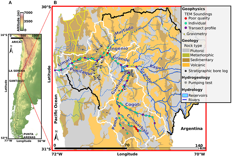
Figure 1. Study area. (A) Overview map indicating the Limarí catchment location in north-central Chile. Elevation map from ASTER GDEM. (B) Detailed map of the Limarí catchment (black solid line) and of the area of study (white solid line) showing the main rivers and reservoirs as well as the geophysical, geological, and hydrogeological data locations. The geology map is from Servicio Nacional de Geología y Minería (2003), where the volcanic rock type includes volcanic-sedimentary formations.

Geophysical methods are well-established for the characterization of groundwater reserves (Kirsch, R., 2009). In particular, electromagnetic methods such as transient electromagnetic sounding (TEM; Fitterman and Stewart, 1986; Auken et al., 2003; Christiansen et al., 2009) are well-suited for the characterization of unconsolidated sedimentary aquifers. From TEM measurements it is possible to infer plausible vertical 1D models of the subsurface electrical resistivity and its distributions, which can then be interpreted in terms of geological material (especially if correlated with stratigraphic bore logs). Furthermore, electrical resistivity of rock and soils is strongly affected by the water content and its chemistry (Lesmes and Friedman, 2005), so that TEM has been extensively used for groundwater characterization (Ruthsatz et al., 2018; Valois et al., 2018), and its usefulness has already been proved in arid and semi-arid areas (Guerin et al., 2001; Boucher et al., 2009; Descloitres et al., 2013; Viguier et al., 2018; Flores Avilés et al., 2020). Nevertheless, the use of TEM in the study area was potentially challenging because of the high urbanization of the transversal valleys, which can induce electromagnetic noise, and the electrically-resistive plutonic and volcanic environment of the Andes mountain range. Moreover, the known high concentration of sulfates and chlorides of surface water chemistry in some parts of the valley raised a non-unique problem when interpreting electrical resistivity profiles, stressing the need for complementary information such as stratigraphic bore logs, water electrical conductivity measurements, pumping tests and water table depth.

In order to fully characterize the aquifers it was necessary to implement a multidisciplinary approach. Previous studies, also in Andean basins, have shown that the integration of various source of information (i.e., geological, hydrogeological, geophysical, geomorphological, etc.) can contribute to the understanding of the functioning and structure of complex hydrogeological systems. For instance, in Bolivia, Guerin et al. (2001) combined data from TEM soundings and stratigraphic columns to characterize the geometry of the aquifer in the central Altiplano and identify saline groundwater; Gomez et al. (2019) studied the Challapampa alluvial aquifer thickness and bedrock structure through electrical resistivity tomography (ERT) and TEM soundings; Gonzales Amaya et al. (2019) used hydrogeophysics to refine hydrogeological conceptual models; and Flores Avilés et al. (2020) integrated TEM, piezometric and geochemical data together with geological, lithological, and topographic information for the characterization of the Katari-Lago Menor Basin aquifer. Furthermore, in Argentina, Maldonado et al. (2018) incorporated hydrogeochemical and groundwater level data to assess the geochemistry, water flow dynamic and renewal rates of groundwater in deep aquifers of the Pampean plain, while in the northern part of Chile. Viguier et al. (2018) assessed the geometry, boundaries and preferential recharge zones of an over-exploited aquifer in the Atacama Desert correlating piezometric measurements, TEM soundings and stream gauging.

In the same spirit, this study proposes a suitable multidisciplinary approach for the characterization of steep gradient valley-fill aquifers within a heterogeneous geomorphology setting, resulting in a complex sedimentary system at the scale of the catchment. The aim is to characterize the catchment hydrostratigraphy (i.e., mapping aquifers and confining layers and characterizing aquifer heterogeneity and groundwater chemistry; Maxey, 1964) and to estimate the amount of groundwater stored. We focus on the Limarí catchment as a case study. We carried out two geophysical field campaigns with TEM sounding within part of the catchment (white solid line in Figure 1B), covering its entire topographic span (i.e., from the coast to the high mountain range) and including the sub-catchments of Cogotí, Combarbalá, and Pama rivers, which are the most affected by water scarcity (Flores and Aliaga, 2020). We incorporated stratigraphic and pumping test information, as well as the depth to the water table obtained from an existing groundwater flow model (Flores and Aliaga, 2020). Moreover, we considered surface water quality information (due to the lack of available groundwater conductivity data) and took into account that near the villages of most of the catchment, groundwater is drinkable, meaning that its electrical conductivity is not so impacted by salinity. However, in the western part of the catchment, groundwater salinity increases. Anyway, further hydrogeological studies should also focus on water quality analysis to get a more complete picture of its electrical conductivity distribution. We also considered an existing basin geometry model (Luis et al., 2019) and previous gravimetry datasets (GCF Ingenieros, 2015; Hidrogestion, 2021) to validate the information about the depth of the bedrock inferred from the resistivity models when the TEM exploration depth reached the bedrock, and as complementary information otherwise. Finally, we reviewed and incorporated information about the geomorphology, geology, hydrogeology and groundwater quality of the catchment (SERPLAC et al., 1979; DGA, 2008; Salazar-Gutierrez, 2012; GCF Ingenieros, 2015; Luis et al., 2019; Flores and Aliaga, 2020; Ramos, 2020; Hidrogestion, 2021). We organized and interpreted the results in 10 sectors of hydrogeological continuity defined according to the geomorphology, hydrography and the results of individual TEM soundings (Figure 4A). In each of these sectors, we performed a spatially constrained inversion (SCI of the TEM data) and built 3D resistivity layers-models using 2D kriging interpolation (Krige, 1951) of the inverted TEM model parameters and stratigraphy logs. Finally, we derived estimates of the volume of water stored in each sector.

2. Study Area

The study area (white solid line in Figure 1B) lies in the Limarí catchment (Coquimbo region, Chile), which covers an area of approximately 11,700 km² (black solid line in Figure 1B; Luis et al., 2019). The Limarí river starts at the confluence of the rivers Grande (from the south, draining an area of ~ 6, 537km²) and Hurtado (from the north, draining an area of ~ 2, 600 km²). Both rivers have their origin in the high mountains. The Grande river has two main tributaries: Rapel and Guatulame rivers. In turn, the Guatulame river has three main tributaries: Pama, Combarabalá, Cogotí rivers. Other two important tributaries of the Limarí river, downstream of Ovalle, are the Ingenio and Punitaqui rivers (GeoHidrologia Consultores Ltd., 2016). The catchment hydrology is regulated through three artificial reservoirs that were built for drought mitigation: the largest is La Paloma, located at the confluence of Guatulame and Grande rivers; the smallest is Recoleta, located on the Hurtado river; and in between (in terms of size) is Cogotí, located at the confluence of Cogotí and Pama rivers (DGA, 2008).

Climatically, the Coquimbo region is a transition zone, located between the desert and temperate/ Mediterranean climate zones in the north and in the south, respectively. The climate changes with the altitude and distance from the coast and thus it can be divided in three bands from west to east (Luis et al., 2019). The steppe coastal climate, along the Pacific coast until ~ 40 km inland, is characterized by profuse cloudiness, humidity, moderate temperatures and a dry period that lasts between 8 and 9 months of the year. The steppe warm climate, in the central part of the catchment (above 800 m of altitude), is characterized by an absence of clouds and extremely dry air, higher temperatures and lower precipitations than the coast, and repeated periods of droughts. Finally, the temperate-cold high altitude climate, in the mountains above 3,000 m of altitude, is normally characterized by the highest rate of precipitations in the catchment and low temperature. Moreover, climate change has severely affected the area, where the precipitation recorded in rainfall stations shows a progressive decrease between 1912 and 2010 (Fernando Santibáñez et al., 2014).

The analysis of annual precipitations between 1950 and 2016, displays an average between 160 and 240 mm of annual precipitation within the higher altitude area and between 120 and 140 m in the medium altitude and coastal areas (Hidrogestion, 2021). River flows mainly increase both in the warmest months (November and December) and in winter (June, July, and August), which demonstrates that the basin has both nival (in spring-summer, when snow and ice melt) and pluvial (in winter) contributions (Hidrogestion, 2021).

Six geomorphological macro-units can be identified in the study area (Figure 2; Luis et al., 2019). Here we give a brief description of these units from the west to the east (i.e., with increasing elevation). The littoral plain includes beaches, eroded rock outcrops and ancient marine terraces. The pediplanes of the coastal mountain range correspond to gently sloping surfaces associated with areas where different drainage networks converge or with continental sedimentation plains. They are formed by continental and fluvial sediments deposited by tributaries, accumulation of alluvial fill and receding slopes (Börgel, 1983). The coastal mountain range is mostly made up by plutonic rock with a minor presence of volcanic-sedimentary rocks, both of Cretaceous age. The transversal mountain belt with its pediplanes is a transition zone between the coastal and Andes mountain ranges and is generally composed of volcanic and continental sedimentary rocks. The Andes mountain range is the macro-unit with the largest distribution and the highest altitude (with a maximum close to 6,000 m a.s.l) in the area. It is composed of plutonic, volcanic and continental sedimentary rocks (Figure 1B; Herbert, 1967; Mpodozis and Cornejo, 1988; Rivano and Sepulveda, 1991; Servicio Nacional de Geología y Minería, 2003; Emparan and Pineda, 2006; Pineda and Emparan, 2006; Pineda and Calderon, 2008). The volcano-sedimentary formations were intruded by plutonic rock of Cretaceous or Tertiary age, generating contact zones and hydro-thermal alterations that provide mineralization of copper, gold, iron, manganese, and mercury (Oyarzun, 2010). Finally, the transversal valleys cross all the main geomorphological units from east to west and form the principal valleys associated with the drainage network of the Limarí river.

FIGURE 2

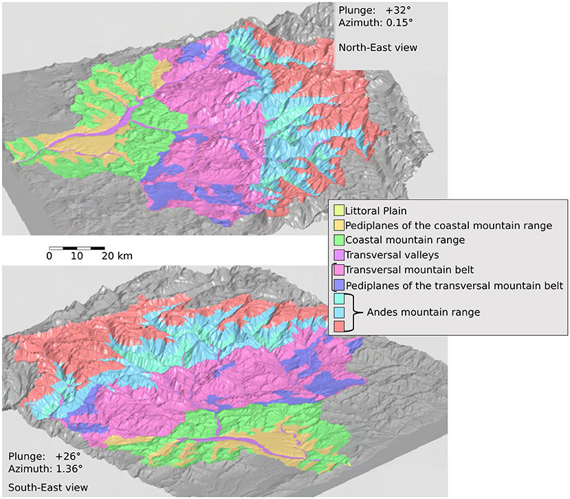
Figure 2. Perspective views of the Limarí river catchment topographic relief. The geomorphological macro-units defined in Luis et al. (2019) are show in different colors. Figure adapted from Luis et al. (2019).

The main unconsolidated sediments present in the study area are alluvial and colluvial deposits together with fluvial (old and modern) and marine terraces. The alluvial deposits mainly form fans at the foot of tributary streams of the main channels. They consist of deposits of poor selection and low compaction made up of gravel, sand and larger blocks immersed in a sand-gravel matrix. Toward the headwaters they merge with colluvial deposits, whereas at their bottom they mesh with fluvial deposits. The colluvial deposits consist of heterogeneous deposits of sand, gravel, blocks, silt and clay of low compaction, which are located in dejection cones, where the sediment distribution varies depending on the slope. The coarse fractions, made up of blocks and gravel in a sand and clay matrix, are mainly located in the apical zone, while in the middle zone the grain size begins to decrease (clayey sands, silts and gravel in a lower extent), and in the bottom zone, they embed with the current alluvial deposits. The old fluvial terraces correspond to steps shaped by the main rivers as they have been deepening their beds. They are mainly made up of blocks, gravel, sand and clay lenses and they are generally thicker and less permeable than the overlaying modern fluvial terraces. The modern fluvial terraces correspond to low compacted sediments that make up the current river beds. They consist of blocks, gravel and sand with some lenses of silty gravel and clay. Finally, in the pediplanes of the coastal mountain range there are four levels of marine terraces associated with changes in sea level during the Pleistocene. These terraces are made up of well-stratified deposits of fluvial-alluvial origin (i.e., sand, gravel, and silt) and they are less permeable than old and modern fluvial deposits due to a larger amount of clay and a larger degree of consolidation (SERPLAC et al., 1979; Salazar-Gutierrez, 2012; GCF Ingenieros, 2015; Hidrogestion, 2021).

Previous studies identified three main aquifer formations in this area (SERPLAC et al., 1979; Salazar-Gutierrez, 2012; GCF Ingenieros, 2015; Hidrogestion, 2021). The unit composed by the Quaternary formations of old and modern fluvial terraces constitutes the most permeable deposit of the catchment. In the pediplanes of the coastal mountain range associated with the Limarí river, these formations overlay the Confluence aquifer formation of late Tertiary age which made up of four levels of terraces associated with changes in sea level during the Pleistocene and composed of well-stratified deposits. It is less permeable than old and modern fluvial deposits, due to its greater amount of clay and its higher degree of consolidation. Finally, in parts of the catchment, the intrusive bedrock presents a high degree of weathering and/or fracturing which can result in significant permeability. The erosion that has created the depressions of the valleys has not occurred in a uniform way. Indeed, rocks of different origin, composition and degree of alteration, have resulted in formation of several concave sectors of substantial depth. Hence, the storage capacity of the volume of valley-fill aquifers is highly variable across the catchment. In this context, the use of a geophysical method with large depth of investigation and sensitive to the contrast between sedimentary filling and bedrock is critical.

3. Materials and Methods

To characterize the aquifer sectors of the study area, we integrated different sources of information: subsurface resistivity models obtained from TEM soundings, stratigraphic bore logs, and previous hydrogeological studies of the Limarí catchment.

3.1. Transient Electromagnetic Sounding

The time-domain or transient electromagnetic (TDEM or TEM) sounding is a controlled-source electromagnetic method that uses transient electromagnetic field diffusion, and is therefore sensitive to changes in the distribution of electrical resistivity in the subsurface (Christiansen et al., 2009). During a TEM sounding, a DC current is passed through a large surface loop (i.e., transmitter loop) generating a static primary magnetic field. Then, the current is interrupted abruptly inducing the collapse of the primary magnetic field. This produces an electromotive force, which in turn creates an induction condition resulting in decaying flowing eddy currents in the subsurface. The intensity of the eddy currents depends upon the resistivity of the subsurface. While propagating, these induced eddy currents produce a time-decaying secondary magnetic field, which in turn induces an eddy current in a surface receiver loop (Fitterman and Stewart, 1986). Compared with resistivity profiles (frequently implemented in groundwater exploration), the TEM method has the advantages of having a larger depth of investigation and requiring a simpler (and faster) field work. However, it only allows for a 1D interpretation of the subsurface resistivity and it presents a restricted sensitivity to intermediate and high resistivity layers (i.e., more than 300 Ωm). Moreover, TEM methods have a decreasing resolution with depth and they lack resolution at very shallow depth (0–5 m, depending on the size of the loop) due to a turn off time delay.

In this study, we used the TEM FAST 48HPC in a coincident-loop configuration, with the same loop acting both as transmitter and receiver. We took a total of 97 soundings in 73 different locations along the main rivers of the study area (Figure 1B). At 19 of these 73 locations, we could perform profiles of more than one sounding transversely to the main river course (i.e., transects depicted as purple circles in Figure 1B) with the aim of characterizing the hydrostratigraphy not only along but also across the main valleys. The spacing between soundings ranges between 1 and 6 km with the high topographic area of the catchment (characterized by heterogeneous sedimentary deposits) presenting an average spacing of 2 km. The soundings were performed with squared loops of side length equal to 25 m (39 soundings), 50 m (55 soundings), or 100 m (3 soundings), where the dimensions were chosen according to field conditions. This leads to a variable depth of investigation (i.e., larger depth of investigation for larger loops in the same subsurface resistivity and noise setting) and different resolution at shallow depth (i.e., the possibility to resolve shallower depth with smaller loops). The measurements were stacked a minimum of 10 times in order to increase the signal-to-noise ratio, and values with a relative noise above 5% were discarded. We discarded 8 measurements due to their large relative noise (represented as red circles in Figure 1B). Six of these points are at the head of the Combarbalá river, where we afterwards discovered that the river is channeled in a PVC tube, which interacts with the induced current as an LCR circuit having an inductive return path to the ground and resulting in an oscillating signal in the TEM measurement. The other two discarded soundings are located one in the Guatulame river and the other in the Limarí river, where in both cases a large electromagnetic noise interfered with the signal.

We interpreted the TEM data with the AarhusInv inversion software (Auken et al., 2015), which implements the 1D discrete model or few layers model (FL), smooth model (SL), and minimum gradient support (MGS) regularizations. In the case of the FL inversion, the software allows for inverting the data for a fixed number of layers with variable thickness, allowing for sharp changes in the resistivity values along the vertical. In contrast, the SL inversion imposes smooth variations in the resistivity between 20 layers of fixed thickness. Finally, the MGS regularization allows for sharp changes in the resistivity values within 20 layers of fixed thickness. The software computes the maximum depth of investigation (DOI) for each sounding according to the inverted resistivity model result, the number of data points within the sounding and their uncertainties (Christiansen and Auken, 2012). In addition, the software provides the option of interpreting different soundings together with a scheme called spatially constrained inversion (SCI), which produces quasi-3D resistivity image using direct 1D solutions (Auken and Christiansen, 2004). With the SCI scheme, the parameters of the 1D models (i.e., resistivity and layer thickness) of nearby soundings are constrained, limiting the lateral variation between the results of the inversion. In this study, we firstly inverted each sounding individually in order to support the identification of sectors of hydrogeological continuity (as explained in details below), and then we implemented the SCI scheme within each sector, with the aim of facilitating lateral coherency of the results and present a general smoothed resistivity model within the different sectors (where the degree of smoothness was tuned accordingly to the complexity of the sedimentary system within each sector). Moreover, in case of sectors presenting TEM soundings at close distance with stratigraphic bore logs, the SCI scheme helps decreasing the ambiguity (i.e., non-uniqueness) in the model results by propagating resistivity model with more prior information in the inversion. Compared to the individual TEM sounding inversion, the SCI leads to a less precise local information (i.e., at the sounding location) but gives an indication of the large degree of resistivity variation at the catchment scale. Moreover, we implemented the laterally constrained inversion scheme (LCI) for the transect profiles. This is a special case of SCI where the constraints are set on a line rather than on a plane (Viezzoli et al., 2008). An example of the different inversion results (individual FL, SL, MGS and spatially constrained FL, SL, MGS) for three TEM soundings of distinct areas of the catchment is given in Figure 3. The examples presented show a general coherence between the results from SCI and individual inversion, especially in case of few layers model. Also, in the higher topographic area of the catchment (e.g., Figure 3A) the 1D resistivity models present a higher degree of similarity between SCI and individual inversion if compared with the lower topographic area of the catchment (e.g., Figure 3C where the higher divergence in the SCI and individual inversion results rise when the MGS and SL scheme are implemented). As explained in more detailed later in this section, this is an effect of the different strength in the constraints implemented in the different area of the catchment in order to take into account the predominant type of sedimentary deposits.

FIGURE 3

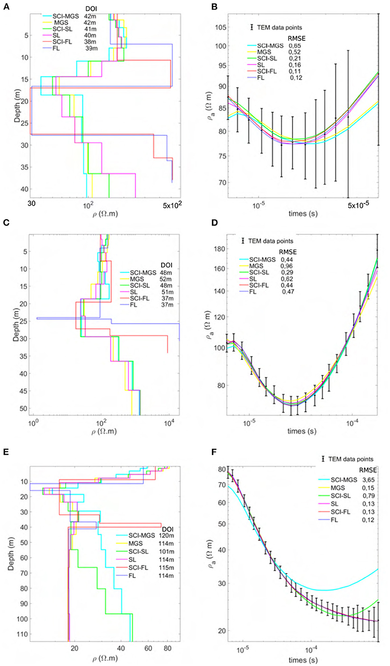
Figure 3. Example of the different inversion scheme results for three TEM soundings in distinct areas of the catchment. (A,C,E) 1D resistivity models; in the text box we show their maximum depth of investigation (DOI). (B,D,F) measured TEM data point and fitted apparent resistivity curves accordingly to the different inversion scheme [minimum gradient support (MGS), smooth model (SL), few layers (FL), individual and spatially constrained inversion (SCI)]; in the legend we give the RMSE value of each inversion scheme result. The measurement points belong to (A,B) the Andes mountain range (Supplementary Figure 2A), (C,D) the transversal mountain range (Supplementary Figure 2D), (E,F) the pediplanes of the coastal mountain range (Figure 8B).

For the hydrostratigraphic interpretation of the resistivity models, we relied on the results of the SCI-FL inversion based on models with five layers. This because these results provided a better fit between the observations and the model responses in comparison to the SCI-SL and SCI-MGS routines (i.e., a smaller root mean squared standardized residuals difference between observations and responses of the models; RMSE). Also, they showed a higher correlation between resistivity and stratigraphic layers from local stratigraphic bore log and the information about depth to the bedrock and subsurface stratigraphy obtained from prior geophysical data (i.e., TEM and gravimetric data; GCF Ingenieros, 2015; Luis et al., 2019; Hidrogestion, 2021). Moreover, within the SCI-FL inversion, the choice of five layers was made after several trials as the least number of layers that allowed the TEM soundings inversion to have a RMSE lower than 2%. Nevertheless, such scheme might lead to thin layers in the model results that shouldn't be resolve by the TEM soundings which has generally a vertical resolution of 10% of the target depth (i.e., approximately 10 m at a depth of 100; Christiansen et al., 2009). For this reason layers thinner than this limits should be consider with care.

We defined 10 sectors of hydrogeological continuity across the sedimentary deposits of the study area based on the geomorphology, hydrography and the individual inversion results of the TEM soundings (Figure 4A). The exact limits were visually defined from aerial photograph and high resolution satellite imagery available on Google Earth (2020). In general, each river section resulted in an individual sector, with the exception of the Limarí and Grande rivers, which both present an element of discontinuity along their path. In the case of the Grande river, the reservoir La Paloma represents both a geomorphological discontinuity and a hydrographic discontinuity. Geomorphologically, although the river belongs to the transversal valleys unit, it crosses the transversal mountain belt above the reservoir and the coastal mountain range below it; while hydrographically, La Paloma represents the confluence of the Grande and Guatulame rivers. In the case of the Limarí river, the geomorphological unit of the coastal mountain range (Altos de Talinay) represents a point of discontinuity: upstream the Limarí river crosses the pediplanes of the coastal mountain range, while downstream it flows through more compact materials, causing the previously wide riverbed to become quite incised until its estuary. For these reasons, these two river basins were each divided into two different sectors of hydrogeological continuity (upstream and downstream of the discontinuity element; Figure 4A).

FIGURE 4

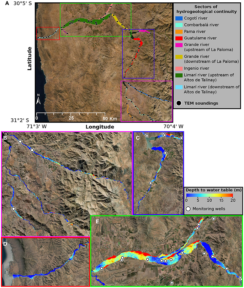
Figure 4. Sectors of hydrogeological continuities and depth to the water table. (A) Overview map indicating the 10 sectors of hydrogeological continuity within the area of study, together with the location of the TEM soundings. (B–E) Depth to the water table obtained from the model Limarí 2020 (Flores and Aliaga, 2020) and DGA monitoring wells locations. Base map images from ESRI World Imagery. (B,C) Sectors crossing the Andes and transversal mountain ranges. (D,E) Sectors crossing the pediplanes of the coastal mountain range, the coastal mountain range and the littoral plain.

Within each hydrogeological continuity sector, we employed the SCI scheme with constraints whose strength (C, dimensionless) depends on the distance between soundings (Viezzoli et al., 2008):

$\begin{array}{ll}C(d)=1+(C_{ref}-1){\left(\frac{d}{d_{ref}}\right)}^a,& (1)\end{array}$

where d is the distance between two constrained soundings, d_ref is the reference distance (in our case the mean distance between soundings within the same sector of hydrogeological continuity) and C_ref is a reference constraint value. The exponent a (regulating how the constraints decrease with the distance and generally ranging between 1 and 2) and C_ref were chosen independently in each sector after several simulations in order to obtain an acceptable fit between observations and model responses and to respect the hydrogeological continuity hypothesis. To determine these two parameters, we set a threshold of 20% as maximum increase of the RMSE between the results obtained through individual inversion and those obtained with the SCI scheme for each TEM sounding. Moreover, we took into account the predominant type of sedimentary deposits in the sectors belonging to different geomorphological domains. For example, we increased a (e.g., up to 2) and decreased C_ref (e.g., down to 0.3) in the narrow valleys of the high mountain ranges where the alluvial and colluvial deposits are expected to be more heterogeneous, and the other way around in the marine terraces of the coastal mountain range pediplanes (e.g., a down to 1 and C_ref up to 0.6).

3.2. Stratigraphic Bore Logs

In order to validate and interpret the electrical resistivity models in terms of lithological material, we revised 141 stratigraphic bore logs available in the study area (black circles in Figure 1B). The depth of these boreholes range from 4.5 to 324 m and its distribution is centered around 65 m. We also incorporated information from the local well cadastre (MOP, 1978) where, although there were no precise GPS locations, it was possible to obtain qualitative information on the lithology of some sectors where other information was lacking. Of the georeferenced stratigraphic logs we were able to compared 41 with nearby TEM soundings in order to correlate resistivity ranges with lithological materials (as exemplified in Figure 8).

3.3. Previous Hydrogeological Studies

We also incorporated different information from previous regional hydrogeological studies of the Limarí catchment, focusing especially on the most recent: the study on the geometry of the drainage basin carried out by the national geology and mining service of Chile (SERNAGEOMIN; Luis et al., 2019) and the latest updates of the regional groundwater flow model carried out by the governmental water authority of Chile (DGA; Flores and Aliaga, 2020) and by Hidrogestion (2021).

The study by Luis et al. (2019), presents a model of the thickness of the sedimentary fill (i.e., depth to the bedrock) throughout the entire Limarí catchment. This model is based on the collection of previous data from gravimetry and TEM soundings (GCF Ingenieros, 2015) and 1548 gravimetric stations measured by SERNAGEOMIN in the context of this more recent study, together with stratigraphic, geological and geomorphological information of the basin. This model was important to validate the results obtained from the interpretation of TEM soundings when the exploration depth reached the bedrock, and to use it as complementary information when the exploration depth of the TEM did not reach the bedrock. With the same purpose, we reviewed the 1790 gravimetry data (yellow points in Figure 1B) collected by GCF Ingenieros (2015) and Hidrogestion (2021); these do not include the gravimetric stations measured by SERNAGEOMIN because of data privacy policy.

Hidrogestion (2021) and Flores and Aliaga (2020) independently updated the regional groundwater flow model developed by GCF Ingenieros (2015) based on previously available and new hydrological, hydrogeological and geophysical data. In particular, the pumping tests database compiled by Hidrogestion (2021) has been a valuable source of information in the present study (white disks with an inner black circle in Figure 1B). We also calculated the temporal average and the temporal standard deviation of the water table depth over the period of the simulation for both models (1995–2016 for Hidrogestion, 2021 and 1964–2018 for Flores and Aliaga, 2020) and quantified the models uncertainty by comparing the simulated water levels with the water levels measured in monitoring wells (white disks with an inner black circle in Figures 4B–E). The approximate total uncertainty was significantly lower for the model of Flores and Aliaga (2020) with a value of 3.6 m compared to 26.9 m for Hidrogestion (2021). Thus, we chose the model of Flores and Aliaga (2020), referred to as the Limarí 2020 model onward, to estimate the water table depth throughout the study area. This information, beside being part of the characterization of the aquifer sectors, helped in some cases to distinguish between saturated coarse material and dry fine material, which may have similar electrical resistivity signature, especially in case of electrically conductive pore-water. Moreover, the 2D water table layer (i.e., Figures 4B–E) extracted from the model Limarí 2020 is crucial for the estimation of stored groundwater within the different sectors of hydrogeological continuity (see Section 3.5 and Appendix A).

All these previous hydrogeological studies assumed a single aquifer layer ignoring the sedimentary architecture of the different area of the catchment which is an important factor to fully characterize groundwater reserves and hydrogeological processes. The current study aims to enrich these groundwater models by providing information about the vertical sedimentary structure. Also, although they are also based on geophysical TEM surveys, these were focused on a restricted area of the catchment and we could only rely on their inversion results rather than the TEM sounding data itself. For this reason the data obtained from this study were crucial for the hydrostratigraphic characterization described in the following section.

3.4. Hydrostratigraphic Interpretation

Through the interpretation of the TEM measurements and their qualitative correlations with stratigraphic bore logs and information from the available hydrogeological studies, we were able to characterize the hydrostratigraphy of the study area. We performed such characterization for each sector of hydrogeological continuity delineated as explained above (Figure 4A). Even though the 10 sectors belong all to the same geomorphological unit (i.e., the transversal valleys), they cross different geomorphological units: Combarbalá, Cogotí, and Pama river sectors cross the Andes mountain range and part of the transversal mountain belt; the sectors of Guatulame river and Grande river upstream of La Paloma only cross the transversal mountain belt; the sector Grande river downstream La Paloma crosses the coastal mountain range; the sectors of Limarí river upstream Altos de Talinay, Ingenio and Punitaqui river cross the pediplanes of the coastal mountain range; and the sector Limarí river downstream Altos de Talinay crosses the coastal mountain range and the littoral plain (Luis et al., 2019).

From the inversion of the TEM soundings we obtained 89 1D profiles of subsurface electrical resistivity with five layers of variable thicknesses. We interpreted these 1D models in terms of lithological materials, correlating the resistivity profiles with the stratigraphic bore logs and pumping tests available in the proximity of TEM soundings and assuming a good correlation between the resistivity values and the type of lithological material along the same hydrogeological continuity sector. In the absence of lithological information, we referred to the general literature to make such correlation (Telford et al., 1990; Reynolds, 2011; Kirsch, R., 2009). In addition, to improve the interpretation, we incorporated information on the water table depth obtained from the DGA monitoring stations and the Limarí 2020 model (Figures 4B–E) as well as information on groundwater and surface water chemistry, since the electrical resistivity of porous media depends not only on the sediments but also on the electrical conductivity of the pore water, which is related to its chemical composition.

Once the different resistivity layers were interpreted in terms of lithology, we were able to assign ranges of hydraulic properties to the different geological material and therefore to each modeled layer, namely porosity (n), specific yield (S_y), specific storage coefficient (S_s), and hydraulic conductivity (K). The ranges of values for these parameters were built from the literature and are presented in Table 1 (Domenico and Mifflin, 1965; Morris and Johnson, 1967; Freeze and Cherry, 1979; Heath, 1983; Domenico and Schwartz, 1990; Batu, 1998). To each interpreted lithology we then associate the mean values of those ranges and estimate their uncertainties from their bounds (see Section 4.3).

TABLE 1

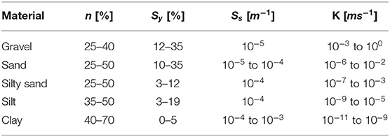
Table 1. Representative values of hydraulic properties for different lithological materials obtained from the literature (Domenico and Mifflin, 1965; Morris and Johnson, 1967; Freeze and Cherry, 1979; Heath, 1983; Domenico and Schwartz, 1990; Batu, 1998).

3.5. 3D Geometrical Reconstruction

In order to build a 3D representation of the resistivity profiles—and thus of the hydrostratigraphic characterization—we followed the methodology of Pryet et al. (2011). I.e., we performed a 2D ordinary kriging interpolation of the depths to layer bottom as well as their resistivity in each sector of hydrogeological continuity. In this procedure we also used additional values of depths to layer bottom derived from the stratigraphic bore log information. To do so, we summarized each log in five layers (compiling sub-sequential layers to a single layer when they presented common material composition) in line with the structure of the interpreted 1D resistivity profiles in the same sector. The interpolation was carried out on an unstructured mesh where each constraining data points has been set as a node, this leading to a varying resolution accordingly to the sector and parameter interpolated (ranging from the order of 1 m² to 1 km²).

In order to implement the 2D kriging interpolation, we computed different empirical semi-variograms for each model parameter of the 10 sectors of hydrogeological continuity and fit them to a different theoretical model (e.g., Figure 5). The general procedure used for the variogram calculation and modeling is hereby resumed in 4 steps:

1. Choice of direction. Natural processes do not lead to isotropic spatial distributions. Typically there is a direction of major continuity (defined through the azimuth) and a direction of minimum continuity perpendicular to it (Deutsch and Journel, 1998). Within each sector we defined the direction of major continuity as the river basin principal orientation in order to compute a directional variogram based on its azimuth.

2. Trend. We investigated the presence of a trend in the conditional data (i.e., the model parameters) by computing a moving window average. When the results showed a significant trend, we subtracted it to the data in order to de-trend them.

3. Experimental variogram computation. For the computation of the empirical variogram, we implemented both a lag and an angle (i.e., azimuth) tolerance in order to account for the limited number of conditional data points and their irregular spacing.

4. Fit variogram model. The choice of variogram model (e.g., power, linear, spherical, exponential, etc.), its parameters (e.g., sill, nugget, lag, etc.) and the tolerance parameters were tuned for the different variograms accordingly to the residuals between the experimental and the modeled variogram. These where optimized in order to have minimum sum and normal distribution. Within the same sector of hydrogeological continuity, we set one variogram model (with different optimized parameters) for all the depths to layer bottom and one for all the layers resistivity.

FIGURE 5

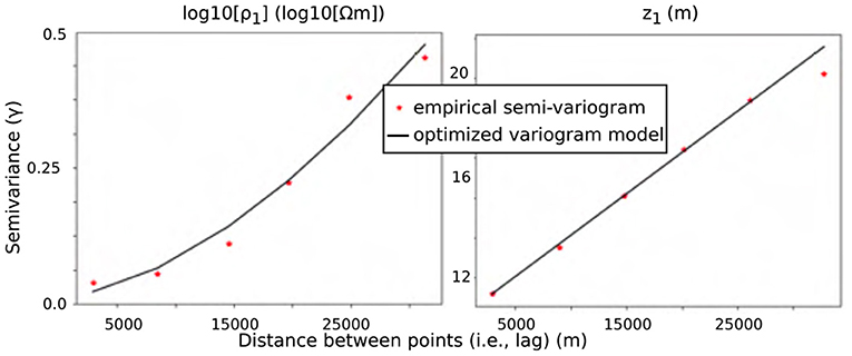
Figure 5. Example of experimental and modeled semi-variogram for the first layer resistivity (ρ₁) and depth to the bottom (z₁) of the sector Limarí river upstream of Altos de Talinay.

In this approach, the uncertainty on the model parameters comes both from the geophysical inversion (i.e., inversion variance ${\sigma }_{INV}^2$) and from the interpolation (i.e., kriging variance ${\sigma }_{KRI}^2$). In the first case, the least-squares inversion criterion implemented in the AarhusInv software provides an estimation of the uncertainty on the model parameters from the propagation of the observational errors into the model covariance matrix (Auken and Christiansen, 2004; Menke, 2012). The other source of uncertainty is quantified by the kriging variance on the interpolated predictions and depends on the spatial variability of the parameters and the distance to the data points. Since these two sources of uncertainty are independent, the total variability on each model parameter (k; i.e., resistivity and depths to layer bottom) is given by:

$\begin{array}{ll}{\sigma }^2\left[k(x,y)\right]={\sigma }_{INV}^2\left[k(x,y)\right]+{\sigma }_{KRI}^2\left[k(x,y)\right],& (2)\end{array}$

In order to evaluate the ability of the kriging interpolator to properly predict the model parameters and their variations, we performed the leave-one-out cross-validation test and checked the root mean squared standardized prediction error for each sector (Isaaks and Srivastava, 1989). All the “measured” values (in our case, the resistivities from the SCI-FL inversion or the layer thicknesses from the SCI-FL inversion and the stratigraphic bore logs) were used to construct the trend and auto-correlation model. Iteratively, each of the measured values location was removed and its value predicted through kriging interpolation of the remaining measured values. For each location (i), it is then possible to compare the measured (z_i) and predicted (${\tilde{z}}_i$) values. Kriging predictions tend to the mean of the values points (Cressie, 1993). In consequence, values far above or far below that mean will tend to be respectively under- and overestimated. This is why in a scatter plot comparing the predicted values with the measured ones, the points will tend to be aligned on a straight line with a slope slightly above 1. The root mean squared standardized prediction error (rmsspe) has equation:

$\begin{array}{ll}rmsspe=\sqrt{\frac{{\displaystyle {\sum }_{i=1}^n}{({\tilde{z}}_i-z_i)}^2}{n{\displaystyle {\sum }_{i=1}^n}{\tilde{\sigma }}_i^2}},& (3)\end{array}$

where n is the number of measured values available in each sector and ${\tilde{\sigma }}_i^2$ is the kriging variance. An error lower than one means that the kriging prediction uncertainty is overestimated, whereas an error higher than one means that it is underestimated.

Once we obtained the 3D layers resistivity model, we were able to upscale the hydrostratigraphic characterization to each sector of hydrogeological continuity. Finally, through the integration of the water table depth, the thickness of the sedimentary filling in the different layers and the distribution of porosity and specific yield within them, we estimated the column of available water across each sector and the total volume of water stored within each sector, together with its uncertainty (see Appendix A for more details about the estimation of volumes and their uncertainty).

4. Results

4.1. TEM Soundings Inversion and Resistivity Interpretation

The results of the SCI-FL inversion are summarized in Tables 2, 3 for each sector. In Table 2, we present the summary statistics of the inversion fits (i.e., RMSE) to show the level of accordance between the SCI-FL inverted model results and the TEM sounding. In Table 3, we present the inverted resistivity values. For each resistivity value, we summed the thicknesses of the layers corresponding to it, obtaining a cumulative thickness; then we computed the relative contribution of four classes of resistivity values to the total layer thickness of each sector and of all sectors for the global results. The defined resistivity classes are:

c1 : ρ ≤ 50 Ωm

c2 : 50 < ρ ≤ 200 Ωm

c3 : 200 < ρ ≤ 1000 Ωm

c4 : ρ > 1000 Ωm.

TABLE 2

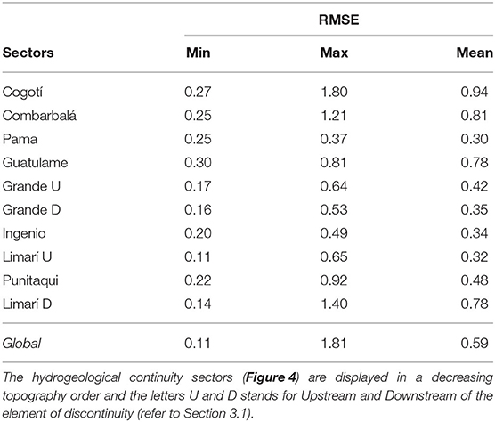
Table 2. Summary statistics of the TEM sounding SCI-FL inversion fit (i.e., root mean squared standardized error; RMSE).

TABLE 3

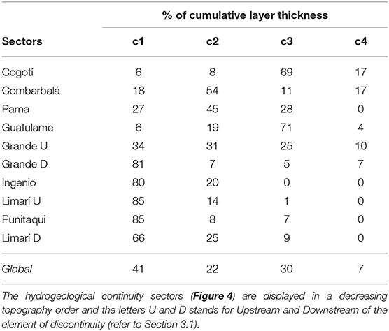
Table 3. Summary statistics of the inverted resistivity values. The percentages correspond to the relative contribution of the resistivity class to the cumulative layer thickness of each sector and of all sectors for the global results.

These classes are chosen so as to provide a relevant summary of the inverted resistivity profiles. The higher resistivity class (ρ > 1, 000Ωm) corresponds to layers where the TEM sounding does not induce current in the subsurface anymore due to the presence of intact sedimentary or plutonic bedrock, for example.

Both tables are organized in a decreasing topography order for the sectors of hydrogeological continuity (from the Andes mountain range to the coast). Furthermore, in Figure 6 we present the inverted resistivity histogram for all the resistivity layers obtained from the SCI-FL inversion of the 89 TEM soundings.

FIGURE 6

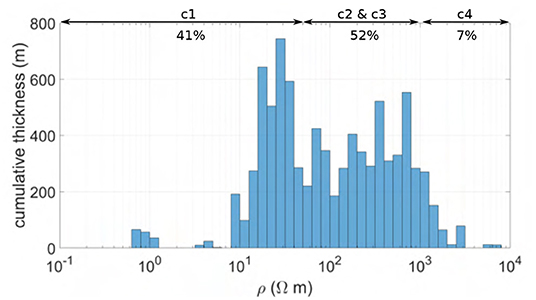
Figure 6. Inverted resistivity histogram for the 89 TEM soundings performed along the whole area of study. The cumulative thickness is the sum of layer thickness corresponding to a specific resistivity range and the percentages correspond to the relative contribution of each class to the cumulative thickness histogram.

The analysis of the cumulative thickness resistivity classes shows two different behaviors. The lower topography part of the catchment, corresponding to the sectors crossing the geomorphological units of the littoral plain, pediplanes of the coastal mountain range and coastal mountain range (Figures 4D,E), presents a predominance of low resistivity values (i.e., class c1); whereas in the higher topography part, corresponding to the sectors crossing the transversal mountain belt and the Andes mountain range (Figures 4B,C), classes c2 and c3 prevail. This behavior is also shown in the global histogram of Figure 6, which displays a bi-modal nature, with a first peak centered around ρ = 30 Ωm and a second one centered around ρ = 350 Ωm. This reflects the thickness of the sedimentary filling and the prevalence of different kinds of deposits across the catchment (beside the low compacted sediments constituting the modern fluvial terraces along the current river beds): thicker sedimentary filling of marine and old fluvial terraces with predominance of impermeable fine material (silt and clay) in the lower part of the catchment, and thinner alluvial and colluvial deposits with less compacted and poorly selected materials presenting a significant percentage of coarser grain deposits (gravel, sand and blocks) in the narrow valleys of the higher mountain range. Moreover, in the western part of the catchment, the electrical resistivity of groundwater decreases due to the high concentration of sulfate and chloride dissolved in the Ingenio and Punitaqui river (GCF Ingenieros, 2015), and the influence of sea water in the Limarí river estuary. This implies that saturated permeable layers also contribute to the predominance of low resistivity values in this part of the catchment.

Figure 7 shows an example of the inverted TEM resistivity results for each of the geomorphological domains represented in Figures 4B–E. Cogotí river, which crosses the Andes mountain range and for a small part the transversal mountain belt; Guatulame river, which crosses the transversal mountain belt; Limarí river upstream of Altos de Talinay, which lays in the pediplanes of the coastal mountain range; and Limarí river downstream of Altos de Talinay, which crosses the coastal mountain range and the littoral plain. The inverted resistivity results, as well as the cumulative resistivity thickness histograms, give a visualization of the different trends in resistivity values in the eastern (Cogotí and Guatulame rivers) and western (Limarí river upstream and downstream of Altos de Talinay) areas of the catchment.

FIGURE 7

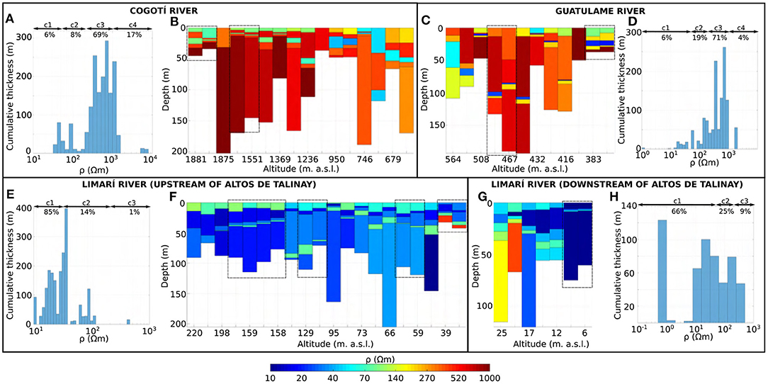
Figure 7. Example of the inverted TEM resistivity results for four sectors of hydrogeological continuity. For each sector are displayed the cumulative resistivity thickness histograms (A,D,E,H) and the inverted 1D resistivity profiles in a decreasing topographic order (B,C,F,G). Within the dashed-line boxes are represented resitivity profiles belonging to the same transect. The sectors displayed are Cogotí (A,B), Guatulame (C,D), and Limarí river upstream (E,F) and downstream (G,H) of Altos de Talinay. Layers with thickness significantly smaller than 10% of their depths should be considered with care.

4.2. Hydrostratigraphic Characterization

As described in Section 3.4, we qualitatively correlated the inverted resistivities from SCI-FL inversion with different lithological materials and their saturation, according to the specific geomorphological, geological, hydrogeological and water chemistry information of each sector. This implies that the same resistivity value can be correlated to different lithological materials in different sectors. In the following, we describe the example of the hydrostratigraphic characterization for the Limarí river upstream of Altos de Talinay, which crosses the pediplanes of the coastal mountain range and belongs to the Confluence aquifer formation (one of the main aquifer formations identified in the study area; Section 2).

The inverted TEM soundings (Figure 7F) together with the geophysical data from previous study in this sector, show a high level of homogeneity along and across this sector. Except for the TEM soundings closest to the Altos de Talinay (two lowest altitude profiles in Figure 7F), no resistivity model reaches the bedrock. The gravimetry data available in this sector show a depth to bedrock of more than 700 m in its deepest part, and between 100 and 300 m in most of the sector. Indeed, apart from the aforementioned TEM soundings, the DOI of the TEM soundings spans between 66.57 and 205.34 m without reaching the bedrock in this sector. Therefore, we relied on the existing gravimetry data to quantify the overall thickness of the sedimentary filling.

To correlate the resistivity layers with different lithological materials, we analyzed the stratigraphic bore logs and pumping tests available. In Figure 8, we present the closest 3 pairs of modeled 1D resistivity profiles and stratigraphic bore logs. Each of these shows a first layer of relatively high resistivity (ρ between 66 and 111 Ωm) correlated with permeable materials (gravel and blocks in Figures 8A,B, and sand in Figure 8C), followed by two lower resistivity layers (ρ between 15 and 30 Ωm) associated with impermeable material (clay). Below that, three stratigraphic columns present a more permeable layer (gravel and blocks in Figure 8C and sand in Figures 8A,B), which is detected in two of the three soundings (those where the DOI reaches it) with an increase in resistivity values (ρ ≈ 70 Ωm in Figures 8C,D). The last layer, detected in two of the three soundings, has lower resistivity (ρ ≈ 15 Ωm) and corresponds to fine impermeable material in the stratigraphic bore logs. From such analysis and the values of inverted resistivity models (Figures 7E,F) we correlated three main lithological materials to three resistivity intervals:

• Clay: ρ ≤ 30 Ωm

• Gravel, blocks and sand: 30 < ρ ≤ 200 Ωm

• Bedrock: ρ > 200 Ωm.

FIGURE 8

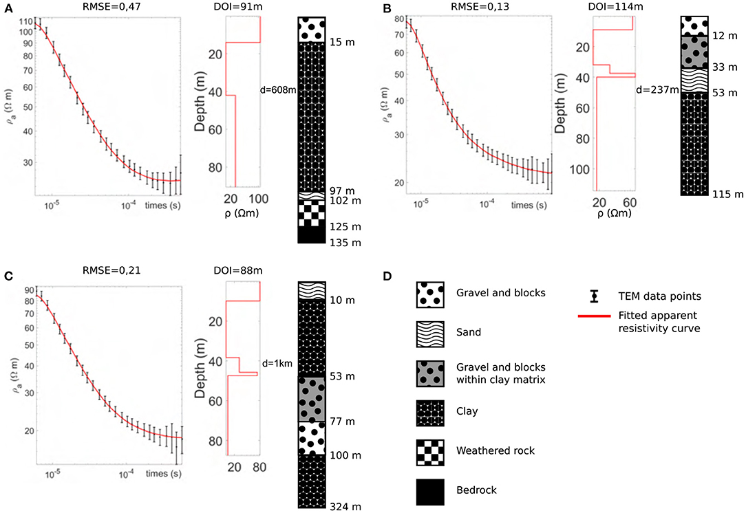
Figure 8. Example of correlation between 1D modeled resistivity obtained from SCI-FL inversion and stratigraphic bore logs in the sector of hydrogeological continuity Limarí river upstream of Altos de Talinay. (A–C) TEM acquired data with fitted apparent resistivity curve and RMSE, 1D resistivity profiles with specified maximum depth of exploration (DOI) and closest bore log with indication of distances, d, between them. (D) Legend of the symbols used.

The lower resistivity values associated to the permeable materials are justified due to the groundwater chemistry alteration of the western part of the sector (from the confluence of Ingenio river downstream). In Figure 9, we summarize the correlation between resistivity and lithological material obtained for the four sectors presented in Figures 7, 10.

FIGURE 9

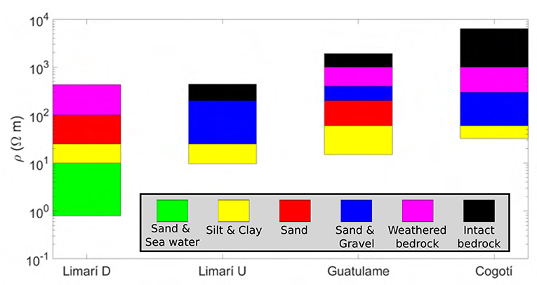
Figure 9. Example of correlation between main lithological materials and resistivity intervals for the four sectors of hidrogeological continuity presented in Figures 7, 10. The sectors are presented in a increasing topographic order. The letter D stands for Downstream of the element of discontinuity (refer to section 3.1).

FIGURE 10

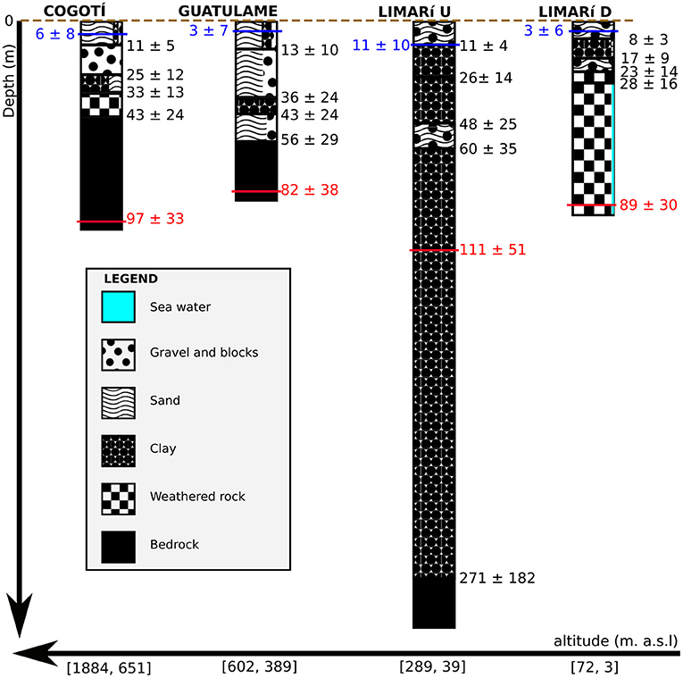
Figure 10. Example of hydrostratigraphic characterizations for four sectors of hydrogeological continuity. The sectors are displayed in a decreasing topographic order. Together with the average depth of the bottom of the modeled layers and their compositions, in blue are represented the average depth to the water table (Figures 4B–E) and in red the average DOI of TEM soundings. Each quantity is given with its total variability which is a combination of its spatial standard deviation and its average uncertainty. The letters U and D stands for Upstream and Downstream of Altos de Talinay.

Data from two pumping tests carried out in the central part of this sector provided hydraulic conductivity values of ≈ 10⁻³ and ≈ 10⁻⁷ m/s, corresponding to gravel and silt, respectively (Table 1). The first value comes from a pumping test of a shallow well (15 m), corresponding to the first identified layer, which is interpreted as permeable material. The second pumping test was performed in a much deeper well (100 m), in which case the hydraulic conductivity must represent an average of the different layers crossed by the well screen, including a large proportion of impermeable material. Hence, our interpretation is in good agreement with the available pumping test data.

We summarized this hydrostratigraphic characterization in Figure 10, where we also represented the characterization done for the sectors Cogotí, Guatulame, and Limarí river downstream of Altos de Talinay, as exemplifications of the four main geomorphological domains of the study area (Figures 4B–E). These results are a summary of the up-scaling of the hydrostratigraphic characterization to the 3D resistivity models (Sections 3.5 and 4.3). For each sector, we displayed the average depth of the bottom of the modeled layers as well as their compositions represented in fractions proportional to the percentage of the different materials across them (e.g., the first layer of Cogotí river sector is composed by 77% of sand, 14% of clay and 9% of gravel and blocks, and is thus depicted with three symbols respecting these proportions). We also reported in blue the average depth to the water table extrapolated from the model Limarí 2020 (Flores and Aliaga, 2020) and in red the average DOI for the TEM soundings. Each quantity is given with its total variability, which is a combination of the spatial standard deviation and the average uncertainty (i.e., Equation 2).

The sectors crossing the Andes and transversal mountain ranges (i.e., Cogotí and Guatulame rivers in Figure 10) display a lower proportion of impermeable material than the sectors crossing the coastal mountain belt (i.e., Limarí river downstream and upstream of Altos de Talinay in Figure 10). This reflects the predominant type of sedimentary deposits in the different geomorphological domains: more heterogeneous and poorly selected alluvial and colluvial deposits in the narrow valleys of the high mountain ranges, and more homogeneous, well-stratified and less permeable deposits of the marine and old fluvial terraces in the lower part of the catchment.

In terms of groundwater resources, the pediplanes of the coastal mountain range present the highest aquifer potential because of their wider surface and the presence of thick confining units that can constitute significant sources of diffuse recharge to the aquifers (Konikow and Neuzil, 2007). Moreover, all the hydrostratigraphic columns (Figure 10 and Supplementary Figures S3–S8) reveal the presence of two permeable sections (i.e., gravel, blocks and sand) separated by one or two impermeable layers (i.e., silt and clay). This is shown also within the other sectors of the basin (see Supplementary Materials). Another key finding of the study is that all the sectors appear to host two aquifers: a superficial unconfined aquifer and a deeper confined (or semi confined) aquifer. However, in the upper sectors of the catchment, the confining unit between the two aquifers appears to be discontinuous.

4.3. 3D Geometrical Reconstruction and Volumes of Water Estimation

As mentioned in Section 3.5, we interpolated the scattered 1D SCI-FL results (i.e., layer resistivities, ρ, and depths to layer bottom, z) in 2D over the area covered by each sector of hydrogeological continuity, also incorporating information from the stratigraphic bore logs available. In Figure 11, we present the case of Limarí river upstream of Altos de Talinay as an example, showing the interpolated layers for ρ and z as well as their uncertainties (σ[ρ] and σ[z]). As already mentioned, the depth to the bedrock was much deeper than the DOI of the TEM soundings in most of the sector, so that we incorporated the information from gravimetric data available as additional points for the 2D kriging interpolation and extended the resistivity values of the 5th layer of the inverted resistivity model to this depth.

FIGURE 11

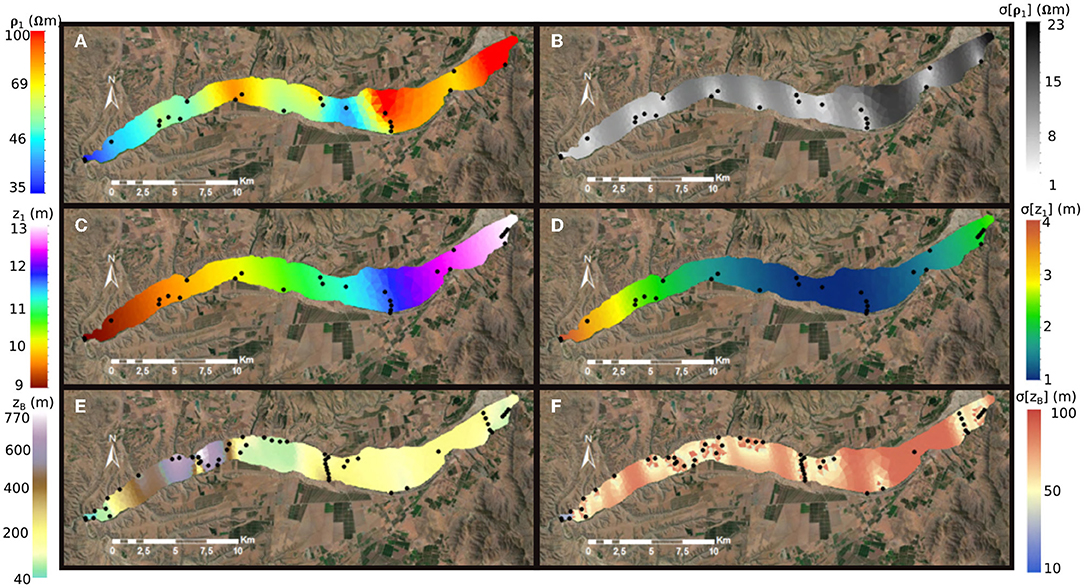
Figure 11. Example of 2D layer interpolation for the sector Limarí river upstream of Altos de Talinay. Interpolated surfaces of the first layer (A) resistivity (ρ₁), (B) resistivity total uncertainty (σ[ρ₁]; from Equation (2)), (C) depth to layer bottom (z₁), and (D) depth to layer bottom total uncertainty (σ[z₁]; from Equation 2). The depth to the bedrock (E) and its total uncertainty (F) were obtained incorporating gravimetry data to the 2D kriging interpolation. For each interpolated quantity we represented the conditioning data location as black dots.

In all the sectors, the major source of uncertainty is from the kriging (i.e., ${\sigma }_{KRI}^2$ is generally larger than ${\sigma }_{INV}^2$ in Equation 2). Note that the error in z increases from one layer to the deeper ones. This is because the inversion parameters obtained from the software AarhusInv are the layer thicknesses, so that the associated errors accumulate when calculating the z of deeper layers. For each sector, and for each layer parameter, we performed the leave-one-out cross-validation test and checked the root mean squared standardized prediction error (Equation 3). We obtained satisfactory results in most of the sectors besides the ones with fewer data points (Punitaqui and Ingenio rivers), where even though they tested well for the leave-one-out cross validation, they all presented a root mean squared standardized prediction error significantly higher than 1 (i.e., between 1.5 and 3), meaning that the kriging variance is underestimated.

From the 3D resistivity model results, we were able to upscale the hydrostratigraphic characterization of the 1D resistivity profiles to the whole area of each sector by correlating the different lithological materials to the defined resistivity ranges, as exemplified in Section 4.2. This allowed us to obtain layers of hydrogeological properties (i.e., n, S_y, S_s and K) estimated as the mean values of the ranges shown in Table 1, together with their uncertainties, estimated from the bounds of the ranges. More specifically, in order to quantify these uncertainties, we considered the uncertainties from the interpolated resistivities and the hydrogeological property ranges of the interpreted lithological material. If, considering the uncertainty on the resistivity (i.e., ρ±σ[ρ]), the resistivity value could be interpreted as two or more different lithological materials, then we increased the uncertainty on the hydrogeological properties to a larger range including all interpreted materials property ranges.

From the interpolated layer thicknesses and the depth to the water table obtained from the groundwater flow model Limarí 2020 (Flores and Aliaga, 2020), we were able to estimate the saturated thickness of each layer (i.e., b_i) and the spatial distribution of the water column stored in it (i.e., the total water column, W_t, based on total, and the available water column, W_a, based on gravitational drainage) for each sector of hydrogeological continuity, together with their uncertainties. Furthermore, we integrated these values over the area delineated by each sector to estimate the volume of water stored in it. The results are showed in Table 4, where we present both the volume of water stored in the whole pore space (V_t) and the amount of available water stored in the specific yield (V_a). Details about the computation of these quantities and associated uncertainties are given in Appendix A.

TABLE 4

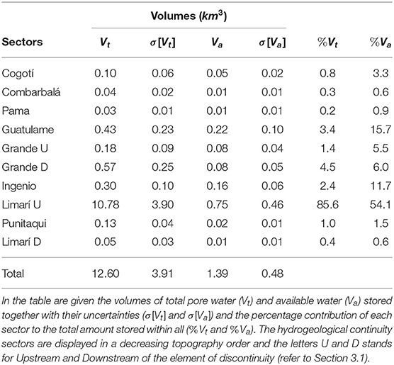
Table 4. Volume of groundwater estimated in the sectors of hydrogeological continuity defined in Figure 4.

5. Discussion

5.1. Resistivity Mapping and Lithological Material

As exemplified in Section 4.2, we were able to qualitatively correlate resistivity ranges to different lithological materials according to the specific geological, geomorphological and hydrogeological setting of each sector. In Figure 12, we visually summarize the material composition of the ten sectors up to the DOI of the TEM soundings. In the figure, we divided the lithological materials in four categories: rock (i.e., weathered or solid bedrock) and three classes of sedimentary deposits according to their grain size (i.e., coarse for blocks, gravel and sand, medium for silty sand and fine for silt, and clay). We also ordered the sectors in four groups (A–D) according to the main geomorphological unit they cross. Within each group, the topography decreases from left to right and from top to bottom in the figure, with the exception of Limarí river downstream of Altos de Talinay, which, despite being the lowest topographic sector (drainage basin estuary), mainly crosses the coastal mountain range, as does the sector Grande river downstream of La Paloma.

FIGURE 12

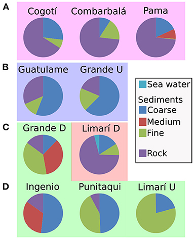
Figure 12. Average material composition for the sectors of hydrogeological continuity. (A) Sectors crossing the Andes mountain range and part of the transversal mountain range. (B) Sectors crossing the transversal mountain range. (C) Sectors crossing the coastal mountain range and the littoral plain. (D) Sectors crossing the pediplanes of the coastal mountain range. The sectors are grouped in shaded boxes according to the color boxes of Figure 4. Sedimentary deposits are divided according to the grain size: coarse (blocks, gravel and sand), medium (silty sand), and fine (silt and clay). The letters U and D stands for Upstream and Downstream of the element of discontinuity (refer to Section 3.1).

With the exception of Limarí river downstream of Altos de Talinay, the main tendency regarding the material composition is an increase in the sedimentary deposits and in the fine material with decreasing topography. This behavior is also reflected in the inverted resistivity values of each sector (i.e., Table 3; e.g., Figure 7). The sectors mainly crossing the Andes mountain range primarily reflect the geology of their bedrock (Figure 1B): the sectors Cogotí and Combarbalá river present the largest percentage of the resistivity class c4 (17%) because of the larger contribution of volcanic and plutonic unweathered bedrock to the resistivity values. The difference between the contributions of classes c2 and c3 (8% c2 and 69% c3 for Cogotí, 54% c2 and 11% c3 for Combarbalá) is a consequence of the major weathering of the bedrock of the Combarbalá sector, which is likely caused by the presence of a normal fault crossing it (Rivano and Sepulveda, 1991; Plummer et al., 2016). For the Pama river sector, a large rock volume is reflected in lower resistivities (28% of class c3 and 45% of class c2) due to the continental-sedimentary composition of its bedrock, which is less resistive in comparison with igneous rocks (Palacky, 1987), and of its weathering (two normal faults cross this sector; Rivano and Sepulveda, 1991). The sectors crossing the transversal mountain belt (i.e., Figure 12B) show a main composition of coarse sedimentary material with a predominance of resistivity classes c2 and c3 (19 and 71% for Guatulame and 31 and 25% for Grande river upstream of La Paloma, respectively). We interpreted the difference in the contribution of class c4 as consequence of the different nature of their bedrock geology: purely igneous (volcanic and plutonic) rocks for the Grande river upstream of La Paloma (10% contribution of c4) and partially sedimentary rocks (in its northern part) for the Guatulame river (4% contribution of c4; Figure 4B). The sectors crossing the coastal mountain range, littoral plain and the pediplanes of the coastal mountain range (i.e., Figures 12C,D) present an increase in the contribution of the resistivity class c1, which corresponds to a significant increase in the composition of medium and fine material in comparison with the higher topography sectors, together with the alteration of the pore water chemistry (as already commented in Section 4.1). Finally, the Limarí river downstream of Altos de Talinay displays a smaller sedimentary filling than the higher topographic sectors. Here the low resistivity values are principally correlated with weathered plutonic bedrock (due to the presence of various normal faults within this sector; Herbert, 1967), electrically conductive pore water and sea water in the deeper layers of the estuary area.

5.2. 3D Resistivity Geometrical Reconstruction and Hydrostratigraphic Characterization Upscaling

For the 3D representation of the scattered 1D resistivity models, we relied on the methodology presented by Pryet et al. (2011), which allowed us to conserve the layer interpretation approach used in the inversion of the TEM data. This scheme has been used in different geophysical studies involving both transient and frequency domain electromagnetic methods, where stratigraphic bore logs information are generally incorporated after carrying out the 3D resistivity modeling as additional information for the characterization of the specific geological target (Christensen et al., 2015; Steinmetz et al., 2015; Valois et al., 2018). Here, we implemented a slightly different approach where we directly incorporated additional layer geometry information in the 2D kriging interpolation based on the stratigraphic information available. When doing this, we firstly summarized each bore log stratigraphy in 5 layers in agreement with the hydrostratigraphic characterization of the sector (e.g., Figure 10), and then incorporated this information as additional data points to the 2D kriging interpolation of the depth to layer bottom. By incorporating these additional data points, the uncertainty on the interpolation results is reduced.

We used the 3D resistivity model to upscale the hydrostratigraphic characterization and retrieve a 3D hydrogeological property model of the different sectors. This resulted in the distribution of porosity, specific yield, specific storage and hydraulic conductivity together with their uncertainties for each layer. Other relevant parameters can also be easily derived such as layer storativity and transmissivity, which may then be used in groundwater flow models.

An important limitation shared by the previous hydrogeological studies and the regional groundwater flow models of Flores and Aliaga (2020) and Hidrogestion (2021) is the assumption of a single aquifer layer that ignores the vertical hydrostratigraphic structure of the sedimentary deposits. The sedimentary structure characterization resulting from our study can be used to improve these models, especially by considering the two aquifer layers identified across the majority of the sectors.

5.3. Water Storage

In Figure 13, we represented the estimated mean values of the water columns for (a) the totality of the pore water and (b) the available water as function of the average altitude of the sector. The values are displayed with horizontal error bars representing the full topographic span and vertical error bars corresponding to their total variability, which is a combination of the standard deviation of the water column in the sector and its average uncertainty. The sectors are grouped in shadow boxes coinciding with the ones of Figure 12 and symbolizing different topographic and geomorphological domains. For the case of pore water columns, there is a significant difference between the average contribution of Limarí river upstream of Altos de Talinay and all the other sectors (more than twice the other average values), especially when compared with the drainage basin estuary (red-shadow box; smaller by a factor of ≈ 15) and the Andes mountain range (magenta-shadow box; smaller by factors of ≈ 12 and ≈ 19). There is also a considerable difference between the larger average values of the pediplanes of the coastal mountain range, transversal and coastal mountain belt sectors (excluding the Limarí river downstream of Altos de Talinay; i.e., green and blue-shadow boxes) when compared with the estuary and Andes mountain range parts of the catchment. Both of these gaps decrease when considering the available water column, where the maximum averaged value is obtained in the Ingenio river sector. Its average pore water column decreases from ≈ 38 m to ≈ 21 m for available water, whereas the average pore water column of the Limarí river upstream of Altos de Talinay decreases from ≈ 140 m to ≈ 10 m for available water. This result is a consequence of the lithological material compositions of the sectors (Figure 12). In particular, in the Ingenio river the medium and coarse materials predominate, while in the other case the fine material (i.e., clay) predominates.

FIGURE 13

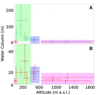
Figure 13. Mean values of the water column distribution for the ten sectors of hydrogeological continuity. (A) Pore water columns. (B) Available water columns. The sectors are grouped in shaded boxes accordingly to the color boxes of Figure 4. The horizontal error bars correspond to the full topographic span of each sector and the vertical error bars correspond to the total variability of the water column within each sector, which is a combination of its spatial standard deviation and its average uncertainty (Equation A4).

As explained in Section 4.3, we computed the volumes of water stored in each sector of hydrogeological continuity by integrating the water column distribution over the corresponding areas (Table 4). The results are coherent with those shown in Figure 13, with the lowest contribution to the water volume from the highest Andes mountain range and drainage basin estuary sectors and the highest contribution from the Limarí river upstream of Altos de Talinay for both the volumes of pore (85,6%) and available water (54,1%). This outcome is a consequence of a thicker saturated sedimentary filling and a larger surface area of the sector Limarí river upstream of Altos de Talinay with respect to the others. This result is in agreement with previous hydrogeological studies (Herbert, 1967; SERPLAC et al., 1979; DGA, 2008; Salazar-Gutierrez, 2012; GCF Ingenieros, 2015; Luis et al., 2019; Flores and Aliaga, 2020; Ramos, 2020; Hidrogestion, 2021) that identified this sector as hosting the main aquifer of the catchment in terms of water-storing potential. Nevertheless, the upstream alluvial aquifers contribute to a total of ≈ 32 % of the available water and of ≈ 10 % of the pore water stored in the characterized area. The role of these upstream aquifers is crucial in semi-arid Chile because they offer a temporary storage with recessions that can last from a few months to almost 3 years, thereby buffering the high inter-annual precipitation variability (Valois et al., 2020).

When computing the uncertainties associated to the water column and the volume of water stored in the different sectors (see Appendix A), we integrated the contribution of four sources of uncertainties: the uncertainty of the inverted geophysical model parameters and their interpolation (i.e., σ[ρ] and σ[z]; from Equation 2), the uncertainty of the water table depth (σ[z_w]) and the uncertainty of the porosity and specific yield estimates. The main contribution to the total resulting uncertainties comes from both the uncertainty over the thickness of each layer (i.e., from the geophysics and its interpolation) and of the porosity and specific yield estimates. The uncertainties associated with the water column and the volume of water stored in the whole pore space are affected twice more by the thicknesses of the layers than the porosity values. On the other hand, the ones associated with the available water stored show a comparable contribution from the layers thicknesses and the specific yield. A good strategy to reduce the total uncertainty could be to decrease either or both: the uncertainty associated with the porosity and specific yield and with the layer thickness. In the first case, the uncertainty could be reduced by laboratory analyses of undisturbed samples of the sedimentary material, by grain size analysis or by the interpretation of borehole geophysics logs data (Robson, 1993; Missimer and Lopez, 2018). Borehole geophysics logs data would also reduce the uncertainty over the layer thickness by adding constraints to the inversion of TEM soundings and additional points for the interpolation. Furthermore, increasing the number of TEM soundings within each sector would reduce both the inversion and interpolation uncertainties over the layer thickness (see Section 5.4).

5.4. Methods and Results Limitation

The main limitation of this study is the restricted number of TEM data points and stratigraphic bore logs. The main limiting factors regarding the number of TEM data points were the time available for the field campaign and the high urbanization of most of the sectors, which reduced the number of possible locations for performing TEM soundings without a significant electromagnetic noise. Regarding the stratigraphic bore logs, we mainly relied on the information available in the groundwater right applications managed by the governmental water authority of Chile. These are particularly scarce in the higher topographic and estuary parts of the catchment, less populated and therefore with less need for groundwater exploitation (and thus drilling). Nevertheless, the limited spatial extension of the sectors and the good correlation between the data points resulted in an acceptable fit of the variograms used for kriging. Furthermore, we incorporated a non-zero nugget to the variogram models in order to avoid large measurement error propagation in the kriging predictions (Goovaerts and Goovaerts, 1997). Still, as mentioned in Section 5.3, additional TEM soundings can improve the SCI inversion results and the interpolation output, decreasing both: the uncertainty on the interpolated model parameters and the kriging variance (therefore the total uncertainty on the resistivity and depths to layer bottom interpolated results), in turn improving the hydrostratigraphic characterization.

In particular, the spacing between the TEM soundings performed is most probably too large (between 1 and 6 km along the main river course) to completely characterize the complex hydrogeological setting. This has been particularly problematic for the headwater sectors crossing the Andes mountain range, where the sedimentary system is made of more heterogeneous and poorly selected alluvial and colluvial deposits. In this case, we expect that the modeled hidrostratigraphic heterogeneity (e.g., Cogotí river in Figure 10) has a much larger wavelength than the real one (i.e., the model shows less complexity than reality). Here, the results of this study should be considered only as general information and additional measurements will be needed for borehole sitting or any local study. Nevertheless, such spacing is likely enough to fully characterize the hydrostratigraphy of the lower part of the catchment (transversal mountain belt and coastal area), which presents a more homogeneous sedimentary system of fluvial and/or marine terraces.

Another limitation of electrical resistivity methods is that they are sensible to both: resistivity of the geological material and water electrical conductivity. As described for the lower part of the catchment, where we found the largest cumulative thickness of low resistivity values (Table 3), we interpreted such low resistivities as an increase in clay content or in salt concentration of the groundwater according to stratigraphic bore logs and water quality information. Nevertheless, as we only have qualitative information about groundwater electrical conductivity, a certain degree of ambiguity remains between impermeable layers with a significant amount of clay and permeable layers filled with salty water. Note that in any case, even though hydrogeologically very distinctive, both outcomes imply that these layers are not suitable for groundwater resources.

Also, the use of literature values for the hydraulic properties assigned to each geological material class (Table 1) led to a large uncertainty in the model results. Moreover, the use of one set of values per geological material, doesn't allow to represent its spatial variability once the resistivity is correlated to a specific material. One perspective of this work that could significantly reduce this uncertainty would be to incorporate information from pumping tests, laboratory analysis and geophysical boreholes measurements (e.g., nuclear magnetic resonance logging; Schmidt and Rempe, 2020) in the quantitative determination of these properties.

Finally, for the computation of water column and volume of water stored in the different sectors, we considered only the sedimentary deposit. Even though we characterized lithological layer of weathered rock, especially in the Andes mountains range and in the estuary part of the drainage basin, there is a large ambiguity between the presence of clay or water in weathered rocks by the sole analysis of electrical resistivity profiles. Hence, the estimate of the (drainable) pore space as well as the hydraulic conductivity or specific storage coefficient must be used with caution in this case.

6. Conclusion and Outlook

The arid and semi-arid regions of the world are facing limited freshwater resources, minimal amounts of rainfall, and increasing population pressure and water demands. Groundwater resources are vulnerable to both natural variability and anthropogenic interventions. In this context a good knowledge of such resources is essential in order to develop sustainable water management strategies.

In this study, we implemented a multidisciplinary approach where we correlated geophysics with geomorphological, geological, hydrogeological data and groundwater quality information to build a 3D hydrostratigraphic representation of various hydrogeological sectors of the Limarí catchment, Chile, and estimate the volume of groundwater stored in their sedimentary deposit.

The derived hydrostratigraphic model can constitute a key input to improve existing regional groundwater flow models, especially by considering the two aquifer layers identified in the majority of the sectors instead of the single aquifer layer implemented in the current models. Our results also confirmed that the Confluence formation in the pediplanes of the coastal mountain range contains a large amount of groundwater stored. The higher altitude areas (sectors crossing the Andes mountain range) host much less groundwater reserves. Nevertheless, the total volume of water stored in these sectors is hydrologically significant, since it can buffer the high inter-annual precipitation variability. Finally, in the coastal range and estuary parts of the catchment, the results show a decrease in groundwater volume and low groundwater quality, with a significant proportion of impermeable material.

Due to the extensive area covered and the large depth of exploration needed, TEM sounding has been a suitable choice for the geophysical prospecting in this study. Initially, we had planned to estimate the groundwater reserve through the use of magnetic resonance sounding (MRS), which gives direct information about the amount of free water (i.e., not bounded to the solid particles surface) in the subsurface as well as the mean size of the water-storing pores (Yaramanci et al., 2005). Nevertheless, the geomagnetic field is close to its global minimum (≈ 23, 000nT; Chulliat et al. in the study area, 2015) and the signal generated by the subsurface water is therefore extremely low, which limits the sensitivity of the method. This fact, together with the high urbanization (and therefore EM noise) of the study area and the presence of magnetic rock, led to an unsuccessful MRS field campaign.

Finally, a follow-up campaign in order to increase the density of local geophysical and hydrogeological survey samples will improve the model results obtained within this study. Adding groundwater electrical conductivity measurements and borehole geophysical multiple-probe logging could improve the quality of the hydrostratigraphic characterization by both measuring different subsurface physical properties (e.g., resistivity, density, gamma radiation, or temperature) and increasing the number of data points used in the geostatistical interpolation. It could also help differentiating the presence of water and/or clay in the weathered bedrock and thereby include this lithological unit in the hydrogeological characterization of the sectors. These data could be used to estimate both porosity and specific yield instead of relying on literature values so to reduce their large uncertainty. Also, for local groundwater well sittings more detailed and local surveys are suggested to integrate the information obtained from this study.

Data Availability Statement

The original contributions presented in the study are included in the article/Supplementary Material, further inquiries can be directed to the corresponding author/s.

Author Contributions

GP ran the inversion, built the 3D model and wrote the manuscript. GP, RV, and PÁ designed the field campaign and the study. GP and EB analyzed the data. RV, EB, and PÁ reviewed the manuscript. All authors contributed to the study. All authors contributed to the article and approved the submitted version.

Funding

This study was supported by CONICYT-FONDEF ProgramaIDeA I+D 2019 (ID19I10001).

Conflict of Interest

The authors declare that the research was conducted in the absence of any commercial or financial relationships that could be construed as a potential conflict of interest.

Publisher's Note

All claims expressed in this article are solely those of the authors and do not necessarily represent those of their affiliated organizations, or those of the publisher, the editors and the reviewers. Any product that may be evaluated in this article, or claim that may be made by its manufacturer, is not guaranteed or endorsed by the publisher.

Acknowledgments

Cristóbal Urquieta, Jeremy Donaire, Micaela Durruty, and Gonzalo Navarro are gratefully acknowledged for their active participation in the field campaign. Also, we would like to thanks the reviewers for helping clarify important points of this study.

Supplementary Material

The Supplementary Material for this article can be found online at: https://www.frontiersin.org/articles/10.3389/frwa.2022.805196/full#supplementary-material

References

Aitken, D., Rivera, D., Godoy-Faundez, A., and Holzapfel, E. (2016). Water scarcity and the impact of the mining and agricultural sectors in Chile. Sustainability 8:128. doi: 10.3390/su8020128

CrossRef Full Text | Google Scholar

Auken, E., and Christiansen, A. (2004). Layered and laterally constrained 2d inversion of resistivity data. Geophysics 69, 752–761. doi: 10.1190/1.1759461

CrossRef Full Text | Google Scholar

Auken, E., Christiansen, A. V., Kirkegaard, C., Fiandaca, G., Schamper, C., Behroozmand, A. A., et al. (2015). An overview of a highly versatile forward and stable inverse algorithm for airborne, ground-based and borehole electromagnetic and electric data. Explorat. Geophys. 46, 223–235. doi: 10.1071/EG13097

CrossRef Full Text | Google Scholar

Auken, E., Jørgensen, F., and Sørensen, K. I. (2003). Large-scale tem investigation for ground-water. Explorat. Geophys. 33, 188–194. doi: 10.1071/EG03188

CrossRef Full Text

Batu, V. (1998). Aquifer Hydraulics: A Comprehensive Guide to Hydrogeologic Data Analysis. New York, NY: John Wiley and Sons.

Google Scholar

Börgel, R. (1983). Geografia de Chile, Tomo II, Geomorfologia. Geografia de Chile, Ediciones Instituto Geografico Militar, Santiago.

Boucher, M., Favreau, G., Descloitres, M., Vouillamoz, J.-M., Massuel, S., Nazoumou, Y., et al. (2009). Contribution of geophysical surveys to groundwater modelling of a porous aquifer in semiarid niger: an overview. Comptes Rendus Geosci. 341, 800–809. doi: 10.1016/j.crte.2009.07.008

CrossRef Full Text | Google Scholar

Chavez, R., Clevers, J., Decuyper, M., de Bruin, S., and Herold, M. (2016). 50 years of water extraction in the pampa del tamarugal basin: can prosopis tamarugo trees survive in the hyper-arid atacama desert (northern Chile)? J. Arid Environ. 124, 292–303. doi: 10.1016/j.jaridenv.2015.09.007

CrossRef Full Text | Google Scholar

Christensen, C. W., Pfaffhuber, A. A., Anschutz, H., and Smaavik, T. F. (2015). Combining airborne electromagnetic and geotechnical data for automated depth to bedrock tracking. J. Appl. Geophys. 119, 178–191. doi: 10.1016/j.jappgeo.2015.05.008

CrossRef Full Text | Google Scholar

Christiansen, A. V., and Auken, E. (2012). A global measure for depth of investigation. Geophysics 77, WB171–WB177. doi: 10.1190/geo2011-0393.1

CrossRef Full Text

Christiansen, A. V., Auken, E., and Saresen, K. (2009). “The transient electromagnetic method,” in ed R. Kirsch Groundwater Geophysics: A Tool for Hydrogeology, 2nd Edn (Berlin: Springer-Verlag), 179–225. doi: 10.1007/3-540-29387-6_6

CrossRef Full Text | Google Scholar

Chulliat, A., Macmillan, S., Alken, P., Beggan, C., Nair, M., Hamilton, B., et al. (2015). The US/UK World Magnetic Model for 2015-2020. BGS and NOAA.

Google Scholar

Cressie, N. (1993). Statistics for Spatial Data. New York, NY: John Wiley and Sons. doi: 10.1002/9781119115151

CrossRef Full Text | Google Scholar

Descloitres, M., Chalikakis, K., Legchenko, A., Moussa, A., Genthon, P., Favreau, G., et al. (2013). Investigation of groundwater resources in the komadugu yobe valley (lake Chad Basin, Niger) using MRS and TDEM methods. J. Afr. Earth Sci. 87, 71–85. doi: 10.1016/j.jafrearsci.2013.07.006

CrossRef Full Text | Google Scholar

Deutsch, C. V., and Journel, A. G. (1998). GSLIB: Geostatistical Software Library and User's Guide, 2nd Edn. New York, NY: Oxford University Press.

DGA (2008). Evaluacion de los Recursos Hidricos Subterraneos de la cuenca del Rio Limari-Informe Tecnico. Ministerio de Obras Publicas- Direccion General De Aguas.

Domenico, P., and Mifflin, M. (1965). Water from low-permeability sediments and land subsidence. Water Resour. Res. 1, 563–576. doi: 10.1029/WR001i004p00563

CrossRef Full Text | Google Scholar

Domenico, P., and Schwartz, F. (1990). Physical and Chemical Hydrogeology. New York, NY: John Wiley and Sons.

Google Scholar

Emparan, C. C., and Pineda, G. F. (2006). Geologia del Area Andacollo-Puerto Aldea, Region de Coquimbo. Carta Geologica de Chile, Servicio Nacional de Geologia y Mineria.

Errázariz, A. M., Cereceda, P., Gonzales, J. I., Gonzales, M., Henriquez, M., and Rioseco, R. (1987). Manual de Geografia de Chile, 3rd Edn. Centro de Informacion de Recursos Naturales, Santiago.

Google Scholar

Favier, V., Falvey, M., Rabatel, A., Praderio, E., and Lopez, D. (2009). Interpreting discrepancies between discharge and precipitation in high-altitude area of Chile's norte chico region (26–32°s). Water Resour. Res. 45, 1–20. doi: 10.1029/2008WR006802

CrossRef Full Text | Google Scholar

Fernando Santibáñez, Q., Paula Santibáñez, V., Carolina Caroca, T., Pablo Morales, P., Paulina González, M., Ninoska Gajardo, A., et al. (2014). Atlas del cambio climatico en las zonas de regimen Arido y semiarido: regiones de Coquimbo, Valparaiso y Metropolitana (Chile). Universidad de Chile, Centro de Agricoltura y Medio Ambiente, Santiago.

Fitterman, D. V., and Stewart, M. T. (1986). Transient electromagnetic sounding for groundwater. Geophysics 51, 995–1005. doi: 10.1190/1.1442158

CrossRef Full Text | Google Scholar

Flores Avilés, G. P., Descloitres, M., Duwig, C., Rossier, Y., Spadini, L., Legchenko, A., et al. (2020). Insight into the Katari-Lago Menor Basin aquifer, Lake Titicaca-Bolivia, inferred from geophysical (TDEM), hydrogeological and geochemical data. J. South Am. Earth Sci. 99, 102479. doi: 10.1016/j.jsames.2019.102479

CrossRef Full Text | Google Scholar

Flores, C. A., and Aliaga, M. A. (2020). Diagnostico del Estado Hidrogeologico de la Cuenca del Limari-Informe Tecnico. Ministerio de Obras Publicas- Direccion General De Aguas-Division de estudios y planificacian.

Freeze, R., and Cherry, J. (1979). Groundwater. Englewood Cliffs, NJ: Prentice Hall.

Google Scholar

Garreaud, R. (2009). The andes climate and weather. Adv. Geosci. 22, 3–11. doi: 10.5194/adgeo,-22-3-2009

CrossRef Full Text | Google Scholar

GCF Ingenieros (2015). Estudio geofisico e hidrogeologico en la cuenca del Rio Limari-Informe Tecnico. Innova Chile CORFO.

GeoHidrologia Consultores, Ltd. (2016). Impacto Aplicacion caudal Ecologico Minimo Retroactivo en Cuenca de la IV, V y VI region. Ministerio de Obras Publicas- Direccion General De Aguas.

Gomez, E., Larsson, M., Dahlin, T., Barmen, G., and Rosberg, J. (2019). Alluvial aquifer thickness and bedrock structure delineation by electromagnetic methods in the highlands of Bolivia. Environ. Earth Sci. 78, 84. doi: 10.1007/s12665-019-8074-x

CrossRef Full Text

Gonzales Amaya, A., Ortiz, J., Duran, A., and Villazon, M. (2019). Hydrogeophysical methods and hydrogeological models: basis for groundwater sustainable management in Valle Alto (Bolivia). Sustain. Water Resour. Manage. 5, 1179–1188. doi: 10.1007/s40899-018-0293-x

CrossRef Full Text | Google Scholar

Google Earth (2020). Eye altitude 3.72 km Maxar Tecnologies, 2012.

Google Scholar

Goovaerts, P., and Goovaerts, D. (1997). Geostatistics for Natural Resources Evaluation. New York, NY: Oxford University Press.

Google Scholar

Guerin, R., Descloitres, M., Coudrain, A., Talbi, A., and Gallaire, R. (2001). Geophysical surveys for identifying saline groundwater in the semi-arid region of the central Altiplano, Bolivia. Hydrol. Process. 15, 3287–3301. doi: 10.1002/hyp.284

CrossRef Full Text | Google Scholar

Heath, R. (1983). Basic Ground-Water Hydrology. Denver, CO: U.S. Geological Survey.

Google Scholar

Herbert, T. B. (1967). Geologia de la Hoja de Ovalle, Provincia de Coquimbo. Carta Geologica de Chile, Instituto de Investigaciones Geologicas.

Hidrogestion (2021). Analisis hidrogeologico para alternativas de ubicacion de pozos en acuiferos cuenca rio Limari con modelacion existente para explotacion de aguas subterreneas en sequia-informe tecnico. Innova Chile CORFO.

IPCC (2021). AR6 Climate Change 2021: The Physical Science Basis. Contribution of Working Group I to the Sixth Assessment Report of the Intergovernmental Panel on Climate Change. Cambridge, UK; New York, NY: Cambridge University Press.

Google Scholar

Isaaks, E. H., and Srivastava, R. M. (1989). An Introduction to Applied Geostatistics. New York, NY: Oxford University Press.

PubMed Abstract | Google Scholar

Jones, P. (1953). Geology and ground-water conditions in the lower valley of the Rio Elqui of Chile. Econ. Geol. 48, 457–491. doi: 10.2113/gsecongeo.48.6.457

CrossRef Full Text | Google Scholar

Kirsch, R. (2009). Groundwater Geophysics: A Tool for Hydrogeology, 2nd Edn. Berlin: Springer. doi: 10.1007/978-3-540-88405-7

CrossRef Full Text | Google Scholar

Koltermann, C., and Gorelick, S. (1996). Heterogeneity in sedimentary deposits: a review of structure-imitating, process-imitating, and descriptive approaches. Water Resour. Res. 32, 2617–2658. doi: 10.1029/96WR00025

CrossRef Full Text | Google Scholar

Konikow, L. F., and Neuzil, C. E. (2007). A method to estimate groundwater depletion from confining layers. Water Resour. Res. 43:W07417. doi: 10.1029/2006WR005597

CrossRef Full Text | Google Scholar

Krige, D. (1951). A statistical approach to some basic mine valuation problems on the witwatersrand. J. Southern Afr. Inst. Mining Metall. 52, 119–139.

Google Scholar

Lesmes, D., and Friedman, S. (2005). “Relationships between the electrical and hydrogeological properties of rocks and soils,” in Hydrogeophysics. Water Science and Technology Library, eds Y. Rubin and S. S. Hubbard (Dodrechct: Springer), 201–213. doi: 10.1007/1-4020-3102-5_4

CrossRef Full Text | Google Scholar

Luis, L. V., Cecilia, D. B., Sandra, H. B., José Luis, C. P., and Felipe, F. C. (2019). Geometria de la cuenca del Rio Limari. Region de coquimbo. Servicio Nacional de Geologia y Mineria.

Maldonado, L., Becher Quinodoz, F., Cabrera, A., Blarasin, M., Lutri, V., Matteoda, E., et al. (2018). Hydrogeochemical features and groundwater renewal rate estimates from deep aquifers in the Pampean plain, Cordoba province, Argentina. J. South Am. Earth Sci. 85, 126–134. doi: 10.1016/j.jsames.2018.05.006

CrossRef Full Text | Google Scholar

Maxey, B. G. (1964). Hydrostratigraphic units. J. Hydrol. 2, 124–129. doi: 10.1016/0022-1694(64)90023-X

CrossRef Full Text | Google Scholar

Menke, W. (2012). Geophysical Data Analysis: Discrete Inverse Theory, 3rd Edn. Boston, MA: Academic Press. doi: 10.1016/B978-0-12-397160-9.00010-2

CrossRef Full Text | Google Scholar

Missimer, T., and Lopez, O. (2018). Laboratory measurement of total porosity in unconsolidated quartz sand by two integrated methods. J. Geol. Geophys. 7:5. doi: 10.4172/2381-8719.1000448

CrossRef Full Text | Google Scholar

MOP (1978). Catastro de pozos iv region. investigacion de recursos hidraulicos en la iv region. Ministerio de obras publicas y transportes, Direccion general de aguas, Departamento de Hidrogeologia.

Google Scholar

Morris, D., and Johnson, A. (1967). Summary of Hydrologic and Physical Properties of Rock and Soil Materials as Analyzed by the Hydrologic Laboratory of the U.S. Geological Survey. Denver, CO: U.S. Geological Survey Water. doi: 10.3133/70197603

CrossRef Full Text | Google Scholar

Mpodozis, C. M., and Cornejo, P. P. (1988). Hoja pisco elqui, region de coquimbo. Carta Geologica de Chile, Servicio Nacional de Geologia y Mineria.

Nichols, G. (2009). Sedimentology and Stratigraphy, 2nd Edn). Chichester: Wiley-Blackwell.

Google Scholar

Núñez, J., Vergara, A., Leyton, C., Metzkes, C., Mancilla, G., and Bettancourt, D. (2017). Reconciling drought vulnerability assessment using a convergent approach: application to water security in the Elqui river basin, north-central Chile. Water 9, 589. doi: 10.3390/w9080589

CrossRef Full Text | Google Scholar

Oyarzun, J., and Oyarzun, R. (2011). Sustainable development threats, inter-sector conflicts and environmental policy requirements in the arid, mining rich, northern Chile territory. Sustain. Dev. 19, 263–274. doi: 10.1002/sd.441

CrossRef Full Text | Google Scholar

Oyarzun, R. (2010). Estudio de caso: Cuenca del Limari, Region de Coquimbo, Chile. Compilacion Resumida de Antecedentes. Centro de Estudios Avanz (CEAZA-ULS).

Oyarzun, R., Oyarzun, J., Fairley, J. P., Nunez, J., Gomez, N., Arumi, J. L., et al. (2017). A simple approach for the analysis of the structural-geologic control of groundwater in an arid rural, mid-mountain, granitic and volcanic-sedimentary terrain: the case of the coquimbo region, north-central Chile. J. Arid Environ. 142, 31–35. doi: 10.1016/j.jaridenv.2017.03.003

CrossRef Full Text | Google Scholar

Palacky, G. (1987). “Resistivity characteristics of geological targets,” in Electromagnetic Methods in Applied Geophysics-Theory, ed M. Nabighian (Tulsa, OK: Society of Exploration Geophysicists), 53–129. doi: 10.1190/1.9781560802631.ch3

CrossRef Full Text | Google Scholar

Pineda, G. F., and Calderon, M. N. (2008). Geologia del Area monte patria-el maqui, region de coquimbo. Carta Geologica de Chile, Servicio Nacional de Geologia y Mineria.

Pineda, G. F., and Emparan, C. C. (2006). Geologia del Area vicuna-pichasca, region de coquimbo. Carta Geologica de Chile, Servicio Nacional de Geologia y Mineria.

PubMed Abstract

Plummer, C. C., Carlson, D. H., and Hammersley, L. (2016). Physical Geology, 15th Edn. New York, NY: McGraw-Hill Education.

Google Scholar

Pourrier, J. (2014). Caractérisation des processus de transferts et d'interactions entre les compartiments hydrologiques, hydrogéologiques et cryosphériques d'un bassin versant andin semi-aride soumis á une forte variabilité climatique (Vallée de l'Elqui-Chili) (theses). Université Montpellier II - Sciences et Techniques du Languedoc, Montpellier, France.

Google Scholar

Pryet, A., Ramm, J., Chiles, J.-P., Auken, E., Deffontaines, B., and Violette, S. (2011). 3D resistivity gridding of large aem datasets: a step toward enhanced geological interpretation. J. Appl. Geophys. 75, 277–283. doi: 10.1016/j.jappgeo.2011.07.006

CrossRef Full Text | Google Scholar

Ramos (2020). Analisis actualizado de la disponibilidad hidrica subterrenea en la cuenca del rio Limari. Memoria para optar al titulo de ingeniero civil ambiental, Universidad de la Serena facultad de ingenieria departamento de minas.

Reynolds, J. M. (2011). An Introduction to Applied and Environmental Geophysics, 2nd Edn. Chichester: Wiley-Blackwell.

Google Scholar

Rivano, S., and Sepulveda, P.-H. (1991). Hoja illapel, region de coquimbo. Carta Geologica de Chile, Servicio Nacional de Geologia y Mineria.

Robson, S. (1993). Techniques for Estimating Specific Yield and Specific Retention from Grain-Size Data and Geophysical Logs from Clastic Bedrock Aquifers. Denver, CO: U.S. Geological Survey Water.

Google Scholar

Ruthsatz, A. D., Sarmiento Flores, A., Diaz, D., Reinoso, P. S., Herrera, C., and Brasse, H. (2018). Joint tem and mt aquifer study in the Atacama desert, north Chile. J. Appl. Geophys. 153, 7–16. doi: 10.1016/j.jappgeo.2018.04.002

CrossRef Full Text | Google Scholar

Salazar-Gutierrez, P. A. (2012). Avances en el conocimiento de la relacion aguas superficiales-aguas subterreneas en la cuenca del Limari, region de Coquimbo. Memoria para optar al titulo de ingeniero civil ambiental. Universidad de la Serena facultad de ingenieria departamento de minas.

Google Scholar

Schmidt, L., and Rempe, D. (2020). Quantifying dynamic water storage in unsaturated bedrock with borehole nuclear magnetic resonance. Geophys. Res. Lett. 47. doi: 10.1029/2020G.L.089600

CrossRef Full Text | Google Scholar

SERPLAC, DGA, ONU, and CORFO. (1979). Hidrogeologia de la Cuenca del Río limarí. Investigación de Recursos Hidráulicos en la IV Región, Proyecto CHI-535.

Servicio Nacional de Geología y Minería (2003). Mapa Geológico de Chile (Escala 1:1.000.000).

Souvignet, M., Oyarzun, R., Verbist, K. M., Gaese, H., and Heinrich, J. (2012). Hydro-meteorological trends in semi-arid north-central Chile (29–32 s): water resources implications for a fragile andean region. Hydrol. Sci. J. 57, 479–495. doi: 10.1080/02626667.2012.665607

CrossRef Full Text | Google Scholar

Steinmetz, D., Winsemann, J., Brandes, C., Siemon, B., Ullmann, A., Wiederhold, H., et al. (2015). Towards an improved geological interpretation of airborne electromagnetic data: a case study from the Cuxhaven Tunnel valley and its neogene host sediments (northwest Germany). Netherlands J. Geosci. 94, 201–227. doi: 10.1017/njg.2014.39

CrossRef Full Text | Google Scholar

Telford, W. M. W., Gedart, L. P., and Sheriff, R. E. (1990). Applied Geophysics, 2nd Edn. London, Cambridge University Press.

Google Scholar

UNCCD (1994). United Nations Convention to Combat Desertification. United Nations.

Google Scholar

Valois, R., MacDonell, S., Cobo, J. H. N., and Maureira-Cortes, H. (2020). Groundwater level trends and recharge event characterization using historical observed data in semi-arid Chile. Hydrol. Sci. J. 65, 597–609. doi: 10.1080/02626667.2020.1711912

CrossRef Full Text | Google Scholar

Valois, R., Vouillamoz, J., Lun, S., and Arnout, L. (2018). Mapping groundwater reserves in northwestern cambodia with the combined use of data from lithologs and time-domain-electromagnetic and magnetic-resonance soundings. Hydrogeol. J. 26, 1187–1200. doi: 10.1007/s10040-018-1726-1

CrossRef Full Text | Google Scholar

Viezzoli, A., Christiansen, A. V., Auken, E., and Sorensen, K. (2008). Quasi-3d modeling of airborne tem data by spatially constrained inversion. Geophysics. 73, F105–F113. doi: 10.1190/1.2895521

CrossRef Full Text | Google Scholar

Viguier, B., Jourde, H., Yunez, G., Lira, E. S., Leonardi, V., Moya, C. E., et al. (2018). Multidisciplinary study for the assessment of the geometry, boundaries and preferential recharge zones of an overexploited aquifer in the atacama desert (Pampa del Tamarugal, northern Chile). J. South Am. Earth Sci. 86, 366–383. doi: 10.1016/j.jsames.2018.05.018

CrossRef Full Text | Google Scholar

Vuille, M., and Milana, J.-P. (2007). High-latitude forcing of regional aridification along the subtropical west coast of south america. Geophys. Res. Let. 34:L23703. doi: 10.1029/2007GL031899

CrossRef Full Text | Google Scholar

Yaramanci, U., Kemna, A., and Vereecken, H. (2005). “Emerging technologies in hydrogeophysics,” in Hydrogeophysics, eds Y. Rubin and S. S. Hubbard (Dordrecht: Springer), 467–486. doi: 10.1007/1-4020-3102-5_16

CrossRef Full Text | Google Scholar

Appendix A: Estimation of Water Columns, Volumes of Waters, and their Uncertainties

We computed the total water column (W_t) and the available water column (W_a) for each pixel of the surface defined by the sectors of hydrogeological continuity as:

$\begin{array}{ll}{W}_t={\displaystyle \sum _{i=1}^5}{b}_i{n}_i;& (\mathrm{A1})\end{array}$

$\begin{array}{ll}{W}_a={\displaystyle \sum _{i=1}^5}{b}_i{S}_{yi};& (\mathrm{A2})\end{array}$

where b_i is the saturated thickness of each layer and n_i and S_yi are the estimated porosity and specific yield. The sources of uncertainty for the computation of the water column are the uncertainties associated with the porosity or specific yield (see Section 4.3) and with the saturated thickness of each modeled layer (i = 1, 2, 3, 4, 5). The uncertainty associated with the saturated thickness (σ[b_i]) is given by the combination of the uncertainty associated with the water table depth (σ[z_w]) and with the depths to layer bottom (σ[z_i]) when the layer is not completely saturated (i.e., when the depth to layer bottom is less than or equal to the water table depth):

$\begin{array}{ll}\sigma \left[b_i\right]=\sqrt{{(\sigma \left[z_w\right])}^2+{(\sigma \left[z_i\right])}^2};& (\mathrm{A3})\end{array}$

otherwise it is given by the uncertainty of the depth to the layer bottom alone. Assuming that the two sources of uncertainty (σ[n_i|S_yi] and σ[b_i]) are independent, the total uncertainty associated with the water column is given by:

$\begin{array}{ll}\sigma \left[W_{t|a}\right]=\sqrt{{\displaystyle \sum _{i=1}^5}\left\{{(b_i\sigma \left[n_i|S_{yi}\right])}^2+{(n_i|S_{yi}\sigma \left[b_i\right])}^2\right\}}.& (\mathrm{A4})\end{array}$

To compute the volume of water stored in each sector, we integrated the column of water over the area delineated by each sector. This was discretised as:

$\begin{array}{ll}{V}_{t|a}=A{\displaystyle \sum _{j=1}^N}{W}_{t|a}^j,& (\mathrm{A5})\end{array}$

where N is the number of pixel in a sector, A is the surface covered by each pixel and $W_{t|a}^j$ is the value of water column for pixel j. The uncertainty associated with the water column in different pixels of the same sector are correlated when the pixels are interpreted as being part of the same lithological unit. In order to simplify the propagation of uncertainties to the volume estimate, we assumed a perfect correlation between all the pixels of a sector and computed it as:

$\begin{array}{ll}\sigma [V_{t|a}]=V_{t|a}{\displaystyle \sum _{j=1}^N}\frac{\sigma [W_{t|a}^j]}{W_{t|a}^j}.& (\mathrm{A6})\end{array}$

This results in a small overestimation of uncertainty (when compared with the total uncertainty associated with the volume of water) in the case of heterogeneous layers. On the other hand, when assuming perfectly uncorrelated pixels, the uncertainty reduces dramatically: between 0.2 and 3% of the volume; whereas with the proposed methodology it ranges between 30 and 80% of the volume (Table 3).