 Narayan K. Shrestha
 Frank Seglenieks
 André G. T. Temgoua
 Armin Dehghan
- Boundary Water Issues Unit, Canadian Center for Inland Waters, National Hydrological Service, Environment and Climate Change Canada, Burlington, ON, Canada
The freshwater resources of the Laurentian Great Lakes basin contribute significantly to the environment and economy of the region. With the impacts of climate change becoming more evident, sustainable management of the freshwater resources of the Laurentian Great Lakes basin is important. This study uses 36 simulations from 6 regional climate models to quantify trends and changes in land-area precipitation and temperature in two future periods (mid-century, 2035–2064 and end-century, 2065–2094) with reference to a baseline period (1951–2005) for two emission scenarios (RCP4.5 and RCP 8.5). Climatic forcings from these 36 simulations are used as input to a calibrated and validated hydrological model to assess changes in land snowpack and actual evapotranspiration, and runoff to lake. Ensemble results show wetter (7 to 15% increase in annual precipitation) and warmer (2.4–5.0°C increase in annual mean temperature) future conditions on GL land areas. Seasonal and monthly changes in precipitation and mean temperature are more sporadic, for instance although precipitation is projected to increase overall, in some scenarios, summer precipitation is expected to decrease. Projected increases in highest one-day precipitation and decreases in number of wet days indicate possible increases in extreme precipitation in future. Minimum temperature is expected to increase in a higher rate than maximum temperature. Ensemble results from the hydrological model show projected decrease in snowpack (29–58%). Similarly, actual evapotranspiration is projected to increase, especially during summer months (up to 0.4 mm/day). Annually, runoff is expected to increase (up to 48% in Superior, 40% in Michigan-Huron, 25% Erie and 28% in Ontario). Seasonal and monthly changes in runoff are more sporadic (e.g., projected decrease up to 17% in Erie subdomain in October). Such contrasting patterns of changes in land hydroclimatology of the GL basin will pose challenges to sustainable management of the water resources of the basin in future.
Introduction
The Laurentian Great Lakes (GL) basin (Figure 1) is one of North America's largest water resources systems with an area of approximately 766,000 km2 (USEPA-GoC, 1995; Quinn, 2003). About one-third of the basin area (about 244,200 km2) comprises five interconnected freshwater lakes (Superior, Michigan, Huron, Erie and Ontario), and together they make the largest unfrozen freshwater lake on Earth in terms of surface area (Larson and Schaetzl, 2001). These GLs are large enough to affect the regional climate system (Notaro et al., 2013).
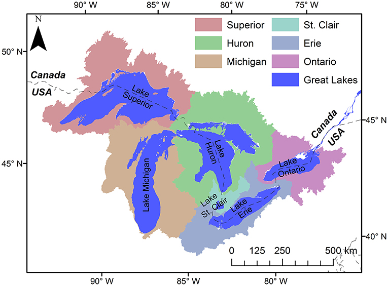
Figure 1. The Laurentian Great Lakes with their respective drainage basin.
The fresh water resources of the GL basin contributes significantly to the environment and economy of the region (ELPC, 2019). More than 30 million people live in the GL basin which includes part of the Canadian province of Ontario and eight United States (U.S.) states; Minnesota, Wisconsin, Illinois, Indiana, Michigan, Ohio, Pennsylvania, and New York. This is about 10 and 30% of the U.S. and Canada's total population, respectively (USEPA, 2021). Many of these people rely on the freshwater resources of the GLs for drinking water, agricultural activities and industrial manufacturing, recreational activities, fisheries, among others (ELPC, 2019). About 20 tribal lands such as Algonkin, Fox, Ho-chunk, Huron, Illinois, Ioway, Iroquois, Kickapoo, Mascounten, Menominee, Miami, Neutral, Nipissing, Ojibwe, Ottawa, Petun, Potawatomi, Santee Dakota, Sauk and Shawnee are also part of the GL basin and the surrounding regions (MPM, 2022). The GLs support several key shoreline wetlands (Mortsch, 1998). Similarly, fisheries in the basin are valued at 7 billion US dollars and recreational activities are estimated to generate about 16 billion US dollars (ELPC, 2019). Hence, sustainable management of the freshwater resources of the GLs is of paramount importance to the people living in the basin (Valiante, 2008).
As a result of the fact that management of the freshwater resources of the GLs is a matter of concern for both Canada and the U.S. (Valiante, 2008), the 1909 Boundary Waters Treaty (BWT) was established with the aim of resolving any water management conflicts between the two states (Whorley, 2020). The International Joint Commission (IJC) was thus established by both governments to make decisions and provide recommendations related to the any projects affecting flows and water levels across the boundary (IJC, 2021). The IJC can issue orders of approval such as Plan 2012 for the regulation of outflow from Lake Superior into Lake Michigan-Huron, and Plan 2014 for the regulation of outflows from Lake Ontario to the St. Lawrence River (IJC, 2021). Through the IJC, coordinated and consistent approaches are being taken to manage the water resources of the GL basin. However, these approaches should also foresee various stressors (e.g., climate change) which are expected to pose a challenge to interests within the GL basin.
Overwhelming evidence suggests that the increase in greenhouse gas concentrations in the atmosphere are unequivocally caused by human activities (IPCC, 2014, 2021). This has led to (a) increase in global surface temperature, (b) increase in frequency and magnitude of extreme precipitation, (c) accelerated glacier retreat, (d) rapid sea level rise, among others. Regional changes in the GL basin could be more extreme than that observed in the global level (IPCC, 2021) and have been driver of various changes in the GL basin (Bartolai et al., 2015). It is thus of paramount importance that an assessment of the impacts of climate change is conducted in the GL basin.
We found about 50 studies that have quantified the impacts of climate change in water resources of the GL basin. The earliest climate change studies in the GL basin used global climate models (GCMs) projections for certain atmospheric CO2 sensitivity experiments such as doubling of the atmospheric CO2 compared to pre-industrial levels to quantify impacts on hydrology (Smith, 1991), net basin supply (NBS) (Cohen, 1986; Croley, 1990), lake level (Marchand et al., 1988; Smith, 1991), lake outflow (Hartmann, 1990), shoreline wetland (Mortsch, 1998) and navigation (Marchand et al., 1988). The NBS is the over-lake precipitation added to the runoff into the lake from its drainage area minus the over-lake evaporation, generally groundwater flow from or into the lake is considered negligible (Fry et al., 2020). During the early years of 21st century, the use of GCM projections with transient climate conditions became more prevalent to quantity the impacts on hydrology (Smith, 1991; Mortsch et al., 2000), ice cover (Lofgren et al., 2002), NBS (Chao, 1999), lake level (Smith, 1991), shoreline community (Schwartz et al., 2004), navigation (Quinn, 2003) and hydroelectric power production (Buttle et al., 2004).
The newer GCMs included earth system feedbacks (e.g., changes in ice sheet, vegetation cover distribution) to project future climate for different Intergovernmental Panel on Climate Change (IPCC) emission scenarios such as the SRES (Special Report on Emissions Scenarios) introduced in the 4th Assessment Report (AR4) (IPCC, 2007) and the RCPs (Representative Concentration Pathways) introduced in the AR5 (IPCC, 2014). Respective Coupled Model Intercomparison Project (CMIP) experiments, the CMIP3 (Meehl et al., 2007) using the SRES and the CMIP5 (Taylor et al., 2011) using the RCPs, provided GCM projections from climatic modeling centers around the world. Some of the climate change studies in the GL basin using IPCC AR4 scenarios quantified impacts on hydrology (Kutzbach et al., 2005; Cherkauer and Sinha, 2010; Rahman et al., 2010), lake level (Angel and Kunkel, 2010; Hayhoe et al., 2010), water quality (Bosch et al., 2014; Hall et al., 2017), ecosystem (Hellmann et al., 2010), infrastructure (Wuebbles et al., 2010) and commercial navigation (Millerd, 2005). Similarly, some of the climate change studies in the GL basin using IPCC AR5 scenarios quantified impacts on hydrology (Wang et al., 2016; Basile et al., 2017; Byun et al., 2019), NBS (Music et al., 2015), lake level (Notaro et al., 2015), fluvial flood risk (Xu et al., 2019), water quality (Cousino et al., 2015; Verma et al., 2015; Wallace et al., 2017) and fisheries industry (Collingsworth et al., 2017).
The impact of GLs on regional climate dynamics is well documented (Notaro et al., 2013). However, the latest GCMs, for example, those participated in the CMIP5 experiments don't explicitly simulate GLs as dynamic lakes (Briley et al., 2021) which may not realistically represent region specific meteorological phenomena such as the lake-effect snowfall (Wright et al., 2013). Therefore, recent studies have used either statistically (Byun et al., 2019) or dynamically (using regional climate models, RCMs) downscaled GCM projections (Notaro et al., 2015; Grady et al., 2021). Furthermore, downscaled projections require bias-correction to remove systematic errors (Cannon, 2018). Downscaled and bias-corrected RCM projections are increasingly being used in the GL basin to quantify impacts on hydrology (Zhang et al., 2018), NBS (Mailhot et al., 2019) and lake level (Mackay and Seglenieks, 2012), among others.
For the North American region encompassing the GL basin, a suite of high resolution downscaled and bias-corrected RCM projections are available through North American component of the Coordinated Regional Downscaling Experiment (Mearns et al., 2017; NA-CORDEX, 2022). It is not a straightforward task to select a set of suitable climate models (Lutz et al., 2016). Cannon (2015) provided guidance on selecting RCMs which can reflect the range of changes in a multi-model ensemble while Lutz et al. (2016) introduced an advanced-envelop based approach. Others argue the use of multi-model ensemble (Crosbie et al., 2011; Acharya et al., 2014) to deal with different sources of uncertainties (e.g., climatic model uncertainty) inherent in RCM projections (Hawkins and Sutton, 2009). Furthermore, the use of a small number of projections in impact analysis may sometimes lead to contrasting results (Smith, 2002). In the GL basin, using projections from 2 GCMs, Lofgren et al. (2002) reported large drops in lake levels when using one GCM input to a hydrological model and moderate increases when using another GCM input. In such cases, inference made through the use of a multi-model ensemble might be more reliable (Krysanova et al., 2018). While using a suite of climate models with different emission scenarios, it is also desirable to estimate the relative contribution of climate model and scenario uncertainty to the total uncertainty in the projected hydrological variable (Lee et al., 2017).
Traditionally, downscaled and bias corrected future projections are used as input to hydrological models to understand the hydrological impacts of climate change (Lofgren et al., 2011). Statistical approaches such as the use of a parametric regular vine copula (VanDeWeghe et al., 2022) are also being advocated as an alternative to the traditional approach. Using the traditional approach, some studies in the GL basin (Lofgren et al., 2011, 2013; Lofgren and Rouhana, 2016; Milly and Dunne, 2017) argued that the use of temperature index (TI) methods such as Thornthwaite (1948) to calculate potential evapotranspiration (PET) in hydrological models creates a hydrological drying bias as TI methods tend to overestimate PET as compared to the methods which respect the surface energy balance. The comparison was based on the PET calculated by hydrological models using input from GCMs to the PET directly simulated by the GCMs. It would be interesting to see if the same holds for bias-corrected downscaled projection from high resolution RCMs. Furthermore, the use of the energy balance approach to estimate PET in a hydrological model is often constrained by the availability of all the incoming and outgoing energy terms in RCM projections. Another issue is that most of the hydrological models are not fully evaluated against all the variables of interest. Assessing the hydrological model performance against a single variable (e.g., streamflow) is more prevalent and it does not guarantee robust simulation of additional variables (e.g., snow water equivalent, SWE; evapotranspiration, ET) (Mai et al., 2021). Similarly, particular to the GL basin, most of the hydrological models don't explicitly consider the impacts of numerous small lakes. The cumulative hydrological impact of these smaller lakes can be substantial in the GL basin (Han et al., 2020).
In this study, we used climatic projections from several RCMs, driven by different GCMs participating in the NA-CORDEX for two IPCC AR5 representative concentration pathways (RCP4.5 and RCP8.5). The RCM projections were bias-corrected using multivariate quantile mapping bias correction technique (Cannon, 2018) using DayMet data (Thornton et al., 2020) as a reference. In total, 36 projections (15 historical, six future for RCP4.5 and 15 future for RCP8.5) at 0.44° (~50 km) spatial resolution were used into a hydrological model. The hydrological model is a coupled model between WATFLOOD (Kouwen, 1988) and RAVEN (Craig et al., 2020) which explicitly considers all lakes with an area more than 5 km2 (Han et al., 2020). Such a coupled model greatly improves the simulation of runoff from the GL basin (Shrestha et al., 2021). Furthermore, the coupled hydrological model is calibrated and validated for daily streamflow, and evaluated against daily SWE and actual ET (Mai et al., 2022). We then quantity the future changes in land hydroclimatic variables such as precipitation, temperature, snow water equivalent (SWE), actual evapotranspiration (AET) and runoff into the lakes.
We presume that quantification of the impacts of climate change on hydroclimatic variables including SWE and AET for the entire GL land basin would be helpful to understand the future hydroclimatic conditions of the GL basin. This may also help to formulate a coordinated effort to address the adverse effects of climate change in the GL basin.
Materials and Methods
Hydrological Model Set-Up
Estimation of vertical hydrological fluxes and their horizontal transfer are two basic processes in a hydrological model (Singh, 1995). The later process is also referred as routing. We used the hydrological model WATFLOOD (Kouwen, 1988) to estimate the vertical fluxes as driven by climatic forcings (e.g., precipitation) and a recently developed lake and river routing product (Han et al., 2020), which has been integrated in the RAVEN modeling framework (Craig et al., 2020). The WATFLOOD model is coupled with the lake and river routing product to realize a functional hydrological model of the GL basin.
Watflood Model
WATFLOOD is a physically-based, distributed hydrological model. In WATFLOOD, a basin is divided into uniform grid cells. Several hydrological processes such as snow accumulation and melt, precipitation interception and infiltration, evaporation and transpiration, surface runoff, interflow and baseflow, etc. are considered for water balance calculations (Kouwen, 1986, 1988; Mai et al., 2021). These calculations are made on grouped response unit (GRUs) which aggregates land cover of similar hydrological response characteristics (Kouwen et al., 1993). WATFLOOD is widely used in hydrological modeling and forecasting of several watersheds in the GL basin and beyond (Cranmer et al., 2001; Seglenieks et al., 2004; Kouwen et al., 2005; Bingeman et al., 2006).
The Lake and River Routing Product Integrated in RAVEN
The GL basin is characterized by the presence of numerous small to large lakes. While larger lakes are usually considered in hydrological modeling, smaller lakes are often neglected. Smaller lakes, when present in a high number as in the GL basin, will impact the streamflow simulations (Han et al., 2020). A lake and river routing product with explicit consideration of all lakes with area more than 5 km2 has become available (Han et al., 2020). Recently, the routing product is integrated into RAVEN modeling framework (Craig et al., 2020), thereby allowing it to run in routing-only mode (RAVEN-ro).
Model Inputs
A 3 arc seconds HydroSHEDS digital elevation model (DEM) (Lehner et al., 2008) and a 30 m North American Land Change Monitoring System (NALCMS) (Homer et al., 2017) landuse/landcover map were used to create the land surface database for the WATFLOOD model. Then hourly precipitation and temperature from a 10 km Regional Deterministic Reanalysis System (RDRS) (Gasset et al., 2021) were used as input into the WATFLOOD model at a 10 km spatial resolution. For modeling purposes, we divided the GL basin in five subdomains: Superior (SUP), Huron (HUR), Michigan (MIC), Erie (ERI) and Ontario (ONT). All input data were obtained in the scope of an on-going project, the Great Lakes Runoff Inter-comparison for Great Lakes, GRIP-GL (Mai et al., 2022). The GRIP-GL is a part of Integrated Modeling Program (IMPC) for Canada under Global Water Future (GWF) program. Related information of the project can be found in http://www.civil.uwaterloo.ca/jmai/projects.html.
We coupled WATFLOOD and RAVEN-based lake and river routing product using the so-called loose coupling scheme (Argent, 2004). Hence, the coupling is one directional in which WATFLOOD simulated runoff (surface and interflow) and recharge to lower zone storage (LZS) are stored in separate netCDF files. These netCDF files then serve as inputs to the RAVEN-ro model. The RAVEN-ro is run to simulate the streamflow at selected locations.
In WATFLOOD, we chose the Hargreaves method (Hargreaves and Samani, 1985) to estimate the rate of potential evapotranspiration. In RAVEN-ro, we chose the Gamma unit hydrograph (RAVEN, 2021) for in-catchment routing and non-linear storage approach for base flow estimation. Outflow from lakes/reservoirs are simulated with a broad-crested weir at their outlet.
In large-scale modeling, it is not always possible to include all the basin complexities (De Scheer et al., 2015). Generally, a compromise in representing these complexities has to be made owing to computation time, data availability, among others. In this study, we also made several simplifying assumptions while setting up the model. In the GL basin, there exist several water bodies which are regulated. Depending on the extent of regulation, these water bodies can have significant downstream impact. The RAVEN-based lake and river routing product incorporates all the significant water bodies and the outflow from these water bodies is simulated using the broad-crested weir equation (Han et al., 2020). Best estimates of all related routing parameters (e.g., weir width, Manning's coefficient, etc.) are already provided in the routing product. During the model calibration, we further fine-tuned some of the important parameters such as the weir width (refer Section Calibration and Validation) to reproduce observed streamflow at immediate downstream gauging stations. We are aware that this (controlling outflow using the broad-crested weir equation) may be too simplified for some of the highly regulated reservoirs in the GL basin, and more detailed approaches such as the use of Dynamically Zoned Target Release (DZTR) (Yassin et al., 2019) may be better suited. A further investigation is needed to confirm this. Another important feature of agricultural water management in the GL basin is the provision of tile drains to quickly drain excess soil moisture after spring snowmelt. Owing to the fact that the tile drainage facilitates the drainage soil moisture in excess of field capacity, we increased relevant parameters (e.g., infiltration coefficient) in agricultural areas to mimic the behavior. This is indeed a simplistic approach and more detailed approaches, such the use of the Hooghoudt and Kirkham drainage equations as incorporated in the Soil and Water Assessment Tool (SWAT) (Neitsch et al., 2011) for explicit consideration of the effect of tile drainage in agricultural areas, may be needed. This issue also needs a detailed investigation. Furthermore, some agricultural areas, especially in the Michigan subdomain, are irrigated. Devoid of detail information regarding the irrigation command area, type, frequency, and amount of irrigation, we did not distinguish irrigated and non-irrigated agricultural areas while setting up the model.
Calibration and Validation
While WATFLOOD was run in an hourly timestep, RAVEN-ro was run in a daily timestep to match the timestep of streamflow observations. The coupled model was calibrated against daily streamflow for a 10-year period (2001–2010) at 134 gauging stations across five subdomains of the GL basin. The model was then validated in another time period (2011–2017) at 59 separate gauging stations (Mai et al., 2022). A total of 17 (11 WATFLOOD and 6 RAVEN-ro related, Supplementary Table S1) parameters were considered during model optimization in the OSTRICH platform (Matott, 2017). We chose dynamically dimensioned search (DDS) (Tolson and Shoemaker, 2007) as an optimization algorithm and Kling-Gupta Efficiency (KGE) (Gupta et al., 2009) as an objective function during optimization. The optimization process resulted in a median KGE of 0.63 during calibration and a median KGE of 0.50 during validation (Mai et al., 2022). For illustration purposes, observed and simulated daily streamflow during calibration and validation periods at two selected gauging stations are shown in Supplementary Figure S1.
We also evaluated the model's robustness in simulating two auxiliary variables, snow water equivalent (SWE) and actual evapotranspiration (AET) (Mai et al., 2022). The Canadian historical SWE station data (CanSWE) (Vionnet et al., 2021) at four selected locations (one station at each sub-domain) were used to compare simulated SWE at the grid exactly over the corresponding CanSWE station. Supplementary Figure S2 shows the resultant plots and it is evident that the model is able to represent the dynamics of SWE at selected stations. The calculated KGE values for daily SWE ranged from 0.48 to 0.70. Similarly, Eddy flux measurements for AET at three AMERIFLUX stations, US-UMB (Gough et al., 2021), US-KM1 (Robertson and Chen, 2021) and US-Oho (Chen et al., 2021) and one FLUXNET Canada Research Network station (Fluxnet Canada, 2016) were used to compare model simulations. The resulting plots for the selected stations are shown in Supplementary Figure S3. The calculated KGE values for daily SWE ranged from 0.52 to 0.73. The median KGE values for SWE and AET are fairly comparable to the KGE values for streamflow. Hence, it is evident that model is equally robust to simulate the SWE and AET dynamics.
Future Climate Data
Future climatic data (precipitation, and maximum and minimum temperature) were downloaded from the National Center for Atmospheric Research (NCAR) climate data gateway (Mearns et al., 2017). These data are projections from different RCMs, driven by several GCMs that participated in the North American component of the Coordinated Regional Downscaling Experiment (NA-CORDEX, 2022). In light of the findings of Briley et al. (2021), it is worth mentioning that only two GCMs (GFDL-ESM2M and HadGEM2-ES, Supplementary Table S2A) simulate GLs as dynamic water bodies, as such, their projections can be considered as “credible”. The remaining 4 GCMs (Supplementary Table S2A) have inconsistency in the treatment of GLs and it mainly arose from “competing or lacking spatial coverage between a model's land and ocean component for grid cell”. As for the RCMs (Supplementary Table S2B), two RCMs (CRCM5-UQAM and RCA4) have the FLake model (Mironov et al., 2009) while one RCM (RegCM4) has the lake model of Hostetler et al. (1993). The two remaining RCMs don't have a standard lake model but they are driven by interpolated and lapse-rate corrected nearby sea-surface temperatures (SSTs) at the lower boundary. It should be noted that the future projections from GCM-RCMs which don't have dynamic representation of GLs might not be as “credible” (Briley et al., 2021). Since the RCM projections were bias-corrected using multivariate quantile mapping bias correction technique (Cannon, 2018) using DayMet data (Thornton et al., 2020) as the reference dataset, the systematic errors are addressed. However, this issue needs further investigation. We used all available RCM projections in both historical (1951–2005) and future (2006–2099) periods at 0.44° (~50 km) spatial resolution. A total of 15 RCM-GCM projections were available in the historical period while 6 future projections were available for RCP4.5 and 15 future projections were available for RCP8.5 emission scenario (Table 1).
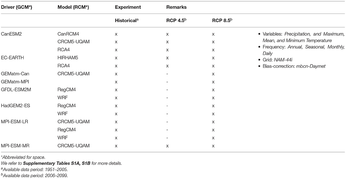
Table 1. Details of the different RCM projections, as driven by different GCMs, used in this study.
The finest temporal resolution of the RCM projections is daily (Table 1), while WATFLOOD needed hourly climatic forcings. Therefore, the daily RCM projections needed to be disaggregated into hourly timestep (Requena et al., 2021). Devoid of a well-accepted procedure to perform such temporal disaggregation, we assumed the total daily rainfall volume to occur in five pulses. With a peak pulse occurring at 8 AM (40% weightage) and another four pulses in 6-hour intervals on either side (at 4 AM and 12 PM both having 20% weighting, and at 12 AM and 4 PM both having 10% weighting). As for temperature, we assumed a linear increase and decrease with daily maximum and minimum temperature occurring at 3 PM and 3 AM, respectively.
For the climate change impact analysis, the entire historical period (1951–2005) was taken as a baseline period. As for the future, a 30-year period (2035–2064) was considered as a mid-century period and another 30-year period (2065–2094) was considered as an end century period.
With regards to the use of hydrological models in climate change impact assessment involving a large number of climate models, Krysanova et al. (2018) detailed two “main” approaches. The first approach advocates using a multi-model ensemble disregarding individual climate model's performance. The proponents of this approach consider every participating climate model as “equal” and argue that an unweighted multi-model approach should be followed (Christensen et al., 2010). The proponents of the second approach advocate in assessing performance of climate models and possibly disregarding poor-performing models. Krysanova et al. (2018) argue that while both approaches have merits and demerits and they are useful in the right context, evaluating performance of a hydrological model in historical period may increase confidence in projected results.
In this study, as we used a hydrological model that was calibrated and validated for streamflow, and evaluated for other auxiliary variables of interests (SWE and AET), we aimed at assessing performance of the hydrological model in representing long-term monthly average streamflow in the historical period. For illustration purpose (Supplementary Figure S4), we selected several gauges (one in each sub-domain) which: (a) are non-regulated, (b) are located closer to the draining lake, and (c) showed a good performance (KGE value more than 0.60) in the calibration period, and (d) have median KGE value more than 0.60 for historical RCM runs for long-term average monthly streamflow. Historical RCM runs are obtained using bias-corrected meteorological forcings in the coupled hydrological model. Furthermore, KGE value for each historical RCM run for long-term average monthly streamflow at all calibration gauges were calculated, and median KGE of the gauges in a specific modeling domain is presented in Supplementary Table S3. For comparison purpose, Supplementary Table S3 also shows the median KGE value obtained in the calibration period.
It is evident from the Supplementary Figure S4, Table S3 that the performance of the model slightly degraded in the historical RCM runs as compared to the performance in the calibration period. A lower performance of the model in another period and for historical RCM runs is indeed expected. While a slight drop in median KGE (calculated from individual KGE values of 21 gauging stations) value for each historical RCM run as compared to a median KGE value obtained during calibration period, is observed in HUR, MIC, ERI and ONT subdomains, a significant drop in performance is observed in Superior sub-domain (SUP) for which median KGE value for each historical RCM run is <0.50 while a median KGE value of 0.77 is obtained during calibration period. The historical RCM runs seem to mimic the seasonality of streamflow, especially the timing and magnitude of the spring peak, in the GL domain as evident in the long-term average monthly plots for selected stations. However, discrepancies are evident in Autumn months. This could be related to several factors such as effectiveness of bias-correction in these months, difference in spatial resolution of the climate forcing (~50 km) and model grids (~10 km) and temporal disaggregation (from daily to hourly, as detailed above) of forcing data.
However, it is evident from the plot (Supplementary Figure S4) and table (Supplementary Table S3) that there is not an obvious poor-performing RCM so that it should be disregarded. Hence, we believe that there is no need to disregard a certain RCMs and all the RCMs were considered for impact assessment.
Uncertainty Analysis
Different sources of uncertainties such as climate model uncertainty and scenario uncertainty are inherent in future climate data (Hawkins and Sutton, 2009). To capture the variability in the future projections, different emission scenarios and several GCM-RCM combinations are often used in climate change impact studies. Relative contribution of different sources of uncertainties to the total uncertainty in the projected hydrological variable is often desirable (Lee et al., 2017). In literature, several approaches are evident. Established approach such as Bayesian decomposition (Ohn et al., 2020) may be more comprehensive but is very time intensive as tens of thousands of iterations may be required which may hinder its application in a large scale physically-based hydrological modeling. A simple yet robust method, based on Maximum Entropy (ME) principle was suggested by Gay and Estrada (2010). Lee et al. (2017) made its first application in hydrological modeling to assess relative contribution of different sources of uncertainty in future streamflow projection in a river basin of South Korea. Because of its robustness and time effectiveness, we also used it to quantify relative contribution of emission scenarios (representative concentration pathways) and climate models uncertainties in total uncertainty of projected SWE, AET and runoff (to the lake). We refer Gay and Estrada (2010) and Lee et al. (2017) for further details of the ME theory and its application in hydrological modeling.
Results and Discussion
Projected Changes in Precipitation
The time series plot of the GL over-land averaged annual precipitation in the historical/baseline period (1951–2005) shows marked variability as indicated by the wide ensemble range (Figure 2). Similar variabilities during a similar historical period were also reported in Do et al. (2020). A Mann-Kendall test (Mann, 1945; Kendall, 1975) shows an increasing trend (p = 0.0003) at 5% significance level. The rate of the increasing trend (0.9 mm/year) is lower than the rate (2.1 mm/year) reported by Bartolai et al. (2015). As for the future periods (mid-century, 2035–2064 and end-century, 2065–2094), a higher variability in annual precipitation is observed for RCP8.5 as compared to RCP4.5, which may be partly due to a higher number of RCM-GCM projections for the RCP8.5 emission scenario. The ensemble mean annual precipitation in both mid- and end-century periods for RCP4.5 shows no trend (p = 0.18, p = 0.35, respectively) at 5% significance level. However, the ensemble mean annual precipitation shows an increasing trend in both mid- and end-century periods for RCP8.5 (p = 0.04, p = 0.03, respectively) at 5% significance level.
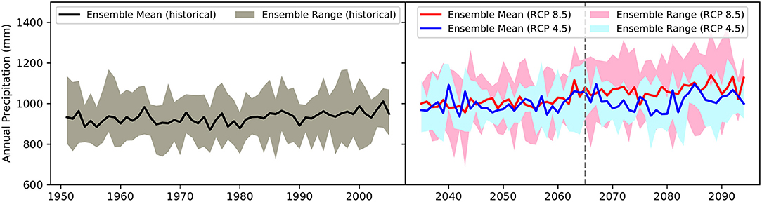
Figure 2. Time series of GL over-land annual precipitation in historical (1951–2005) and future (mid-century: 2035–2064 and end-century: 2065–2094) periods for two emission scenarios (RCP4.5 and 8.5).
While GL over-land ensemble mean annual precipitation do not show any trend (except in the end-century period for RCP 8.5), spatial variability in precipitation trend in different parts of the GL basin is evident in Figure 3. For instance, northern parts of the Lake Huron basin show a decreasing trend of about 2.5 mm/year in the mid-century period for RCP4.5. However, the same region shows an increasing trend of about 3 mm/year in the end-century period for RCP4.5. Similarly, a majority of the Lake Superior subdomain shows a decreasing trend (up to 4 mm/year) in the end-century period for RCP4.5 while the same region in the same period but for RCP8.5 shows an increasing trend (up to 4 mm/year). Such marked spatial variability in future precipitation and contrasting trends in different parts of the GL basin certainty pose challenges to water resources planners and managers and may warrant to focus on sub-basin wise adaptation measures rather than the entire GL basin wide measures.
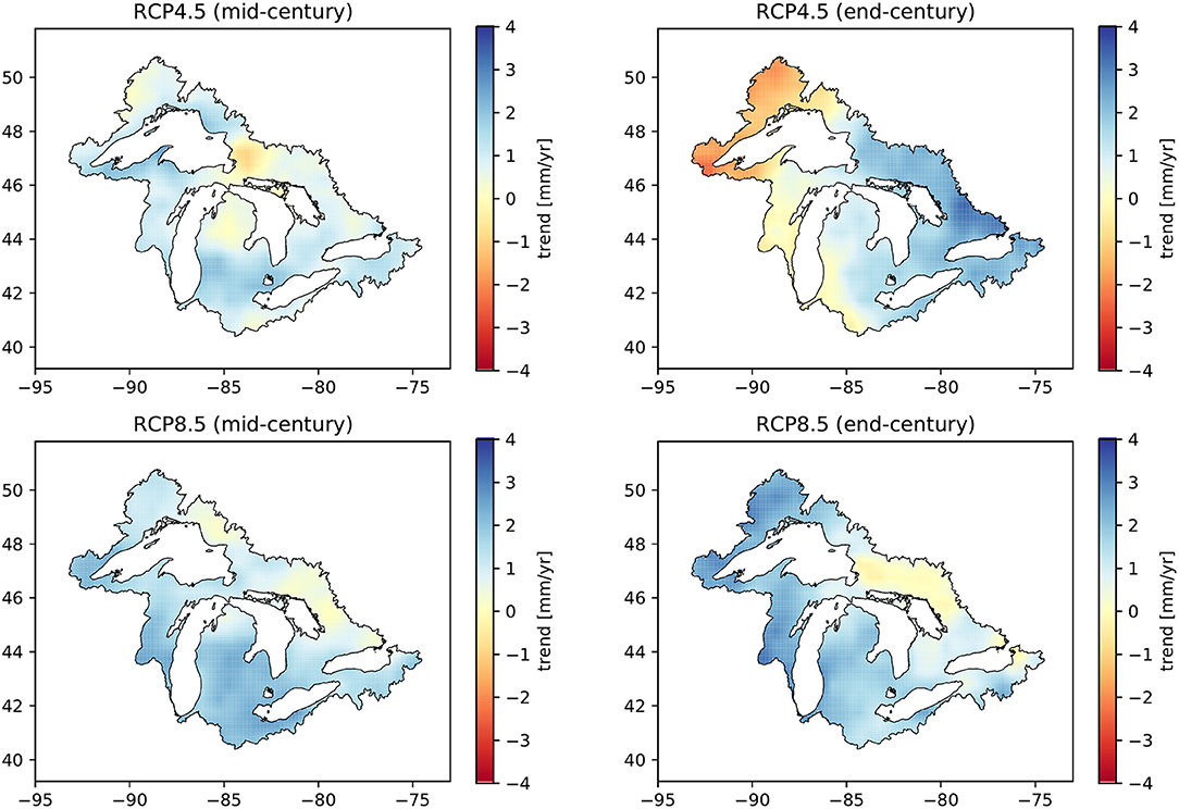
Figure 3. Trend in annual over-land precipitation for RCP4.5 and RCP8.5 scenarios in mid- and end-century periods.
Compared to the baseline annual average precipitation, the projected changes in over-land precipitation can be seen in Figure 4 for both RCP4.5 and RCP8.5 emission scenarios. Besides the spatial variability in future precipitation trends, we observe marked variability in projected annual over-land precipitation amongst the RCM-GCM combinations. For instance, the WRF projections driven by HadGEM2-ES show rather high increases (up to 40%) in future annual precipitation for RCP8.5 scenario while RegCM4 projections driven by MPI-ESM-LR for RCP4.5 seem to indicate decreases for majority of years in both future periods.
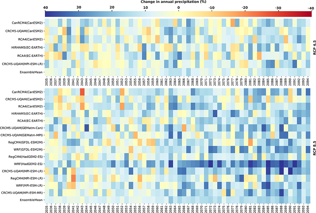
Figure 4. Change in annual over-land precipitation with respect to baseline average precipitation for RCP4.5 and RCP8.5 scenarios in mid- and end-century periods.
On average, the GL land basin is expected to be wetter in future (Figure 5), with annual increases in precipitation range between 7 and 15%. The winter, spring and autumn seasons are expected to have substantial increases (up to 25%). The summer season in contrast, is expected to have a slight decrease (up to 1%) for RCP4.5 emission scenario in the end-century period, due to mild decreases (up to 6%) in August precipitation. The summer precipitation for RCP8.5 scenario is expected to have a slight increase in both future periods (up to 4%). The month of April is expected to have the highest increases (up to 33%). In general, RCP8.5 projections show wetter conditions than RCP4.5, and the same holds for the end-century period as compared to the mid-century period (Figure 5). The general trend in subdomain precipitation changes (Supplementary Figure S5) are almost the same as observed for the entire GL basin except in some months. For instance, in September, the future precipitation is expected to increase in the Superior, Huron and Michigan subdomains while it is expected to decrease in the Erie and Ontario subdomains.
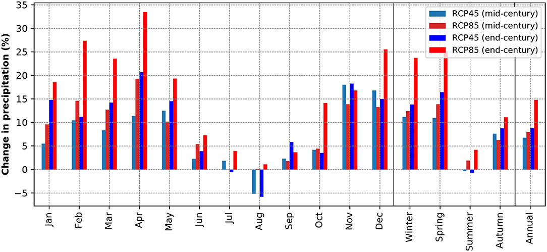
Figure 5. Percentage change in monthly, seasonal, and annual over-land precipitation with respect to the baseline average precipitation for RCP4.5 and RCP8.5 scenarios in mid- and end-century periods.
While a similar result—an overall increase in annual, winter, spring and autumn precipitation and variable summer precipitation was also reported in several studies (Smith, 1991; Cherkauer and Sinha, 2010; Hayhoe et al., 2010; Wuebbles et al., 2010; Byun et al., 2019; Bukovsky and Mearns, 2020; Grady et al., 2021), the magnitude of change is evidently different due to differences in emission scenarios, climate models, bias correction techniques, baseline as well as future periods, and region of interest. For example, Bukovsky and Mearns (2020) used the same dataset (NA-CORDEX, 2022) to analyze seasonal and annual precipitation changes in several regions including the GL basin for RCP8.5 and found very similar results with slight differences in the magnitude of change. For RCP8.5, in mid-century (end-century) period, Bukovsky and Mearns (2020) reported a projected increase in ensemble mean annual precipitation of about 8%(17%) while we found the projected increase to be 8%(15%). Despite the difference in baseline period (1971–1999 in their study vs. 1951–2005 in our study), future periods (mid-century: 2041–2068 in their study vs. 2035–2064 in our study, and end-century: 2071–2099 in their study vs. 2065–2094 in our study), region of interest (entire GL basin in their study vs. only land portion of GL basin in our study) and climate models (28 in their study vs. 15 in our study), the results are very similar.
Projected increases in spring precipitation are certainty concerning as the topsoil in these times of the year will generally be at or near saturation level and any extra precipitation will mostly end up as surface runoff. Similarly, projected decreases in precipitation in the summer months is also concerning from a drought point of view. With expected increases in temperature and higher evaporative demand, future decreases in summer precipitation will only worsen the water stress condition of vegetation, especially, agricultural crops grown in summer. Consequently, crop yield could decrease unless water is supplied to the crops by external means (e.g., surface or sub-surface irrigation).
Further causes of concern are evident in Supplementary Figure S6, which shows projected increases in the frequency of precipitation with daily amounts of more than 5, 10, and 20 mm, and in Supplementary Figure S7, which shows projected increases in highest one-day precipitation. As an example, the highest one-day precipitation in the baseline period is 83 mm (range: 80–93 mm) which is projected to be more than 101 mm (range: 95–112 mm) in the end-century period for RCP8.5. The wider range in projected highest one-day precipitation is also concerning. Furthermore, despite the projected wetter conditions in the GL basin, projected decreases in number of wet days and consecutive wet days indicate that the GL basin is expected to receive more intense precipitation in the future. This increase in intensity could be a concern in regard to flash flooding.
Projected Changes in Temperature
The spread in annual mean temperature from different RCM-GCM combinations in both historical and future periods is narrower (Figure 6) than the spread of annual precipitation (Figure 2). Annual mean temperature of GL basin in the historical period shows a significant (p = 4x10⁻⁹) increasing trend at 5% significance level. The increasing trend persists in mid-century period for RCP4.5 scenario (p = 7 x 10⁻³). The annual mean temperature in the end-century period for RCP4.5 scenario seems to stabilize and shows no-trend (p = 0.20). However, the increasing significant trend persists in both mid-century (p = 1 x 10⁻⁹) and end-century (p = 1 x 10⁻¹⁰) periods for RCP8.5 scenario. The magnitude of the increasing trend in historical period is 0.02°C/year, which increases to 0.03, 0.07, and 0.06°C/year, in mid-century for the RCP4.5 scenario, in mid-century for RCP8.5 and in end-century for the RCP8.5 scenario, respectively.
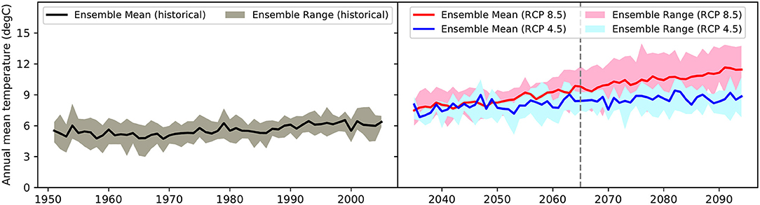
Figure 6. Time series of GL basin annual mean temperature in historical (1951–2005) and future (mid-century: 2035–2064 and end-century: 2065–2094) periods for two emission scenarios (RCP4.5 and 8.5).
Spatially, the trend in annual mean temperature is higher for northern parts of the GL basin (e.g., Superior) than in southern parts (e.g., Ontario) (Figure 7). For instance, in the mid-century period and for RCP4.5 emission scenario, the annual mean temperature in Superior subdomain is expected to increase by 0.04°C/year while for the same period and emission scenario, the Ontario subdomain increase is just 0.02°C/year. While looking at the spatial trends in minimum and maximum temperature (Supplementary Figure S8), the rate of increasing trend of minimum temperature in the GL basin is higher than the rate of increasing trend of maximum temperature in both future periods and for both emission scenarios. Similar findings have been reported by Bartolai et al. (2015) and Kling et al. (2003) in the GL basin.
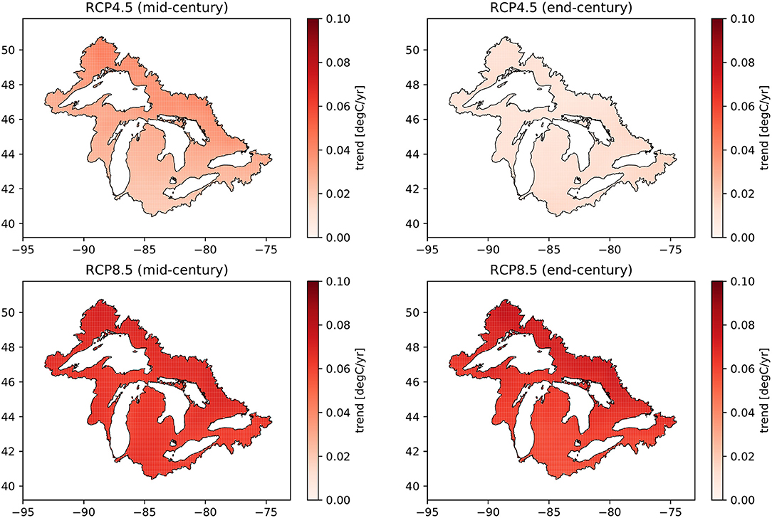
Figure 7. Trend in annual mean temperature of GL basin for RCP4.5 and RCP8.5 scenarios in both mid- and end-century periods.
Relative to the ensemble annual mean temperature in the baseline period, different RCM-GCM projections show a wide range of increases in future annual mean temperature for RCP4.5 and RCP8.5 emission scenarios (Figure 8). In general, future projections for RCP8.5 indicate warmer conditions over the GL basin than for RCP4.5. The same is true for the end-century period as compared to the mid-century period.
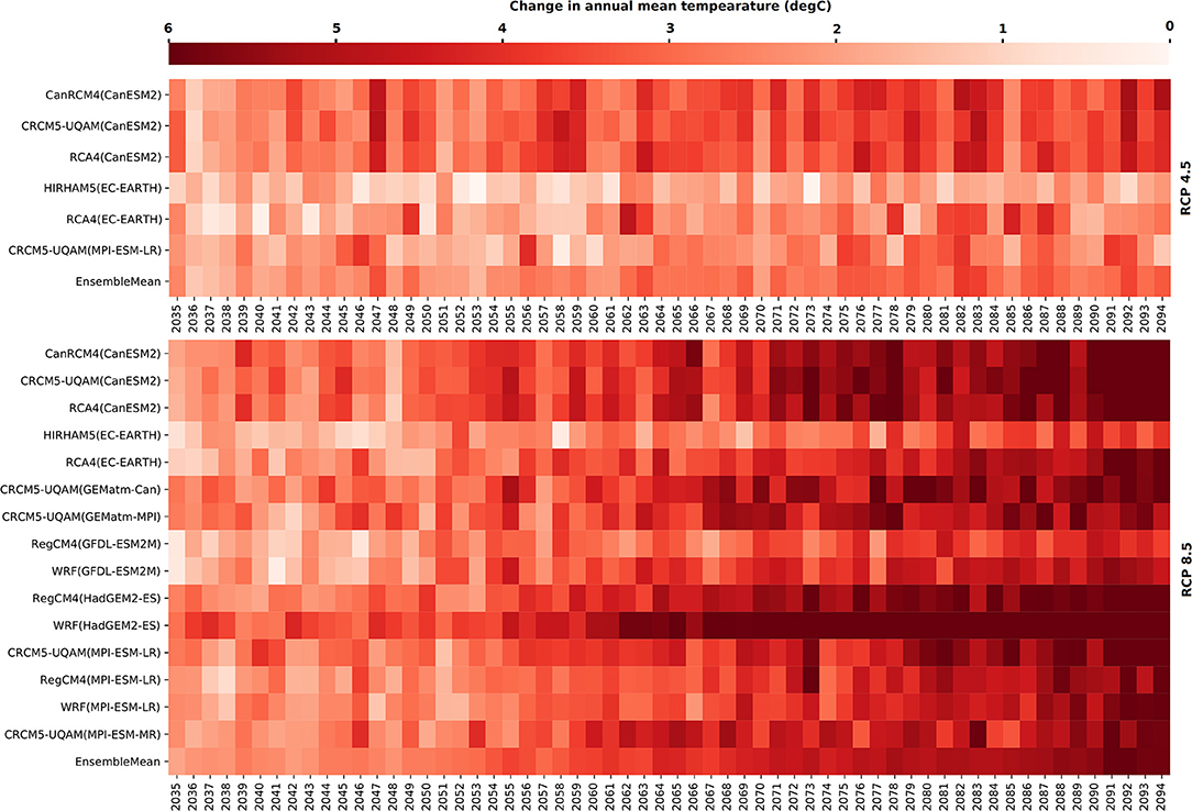
Figure 8. Change in annual mean temperature of GL basin with respect to baseline mean temperature for RCP4.5 and RCP8.5 scenarios in both mid- and end-century periods.
On average, annual mean temperature in the GL basin is expected to increase by 2.4 and 2.9°C, respectively, in mid- and end-century period for RCP4.5 scenario. For the RCP8.5 scenario, the increase is about 3.0 and 5.0°C, in the mid- and end-century periods respectively (Figure 9). In one of the earliest climate change impact assessments of the GL basin, Smith (1991) reported an increase of up to 6.4 oC in annual temperature which is higher than our finding for RCP8.5 in end-century period. However, the estimate made by the study was based on 3 GCMs and for a double (as compared to the preindustrial level) CO2 scenario. However, such a scenario is highly unlikely to occur even at the end of the century. A more direct comparison of our results can be made with the findings of Bukovsky and Mearns (2020) due to the common data source (NA-CORDEX, 2022) and region of interest. For RCP8.5, the study reported the annual ensemble mean temperature changes of about 3.1 and 5.0°C, respectively in mid- and end-century period, which are almost identical to our estimates.
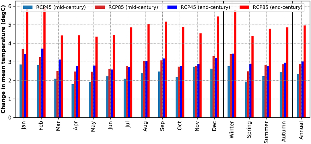
Figure 9. Absolute change in monthly, seasonal, and annual mean temperature of GL basin with respect to baseline mean temperature for RCP 4.5 and RCP 8.5 emission scenarios in both mid- and end-century periods.
Relative to other seasons, the winter season is expected to experience the greatest change, with mean temperature increases reaching up to 5.8°C in end-century period for RCP8.5 scenario. The increase in mean temperature during the spring season is generally less. A similar finding—higher seasonal changes being obscured in annual averages was also reported in several studies (Kling et al., 2003; Kunkel et al., 2009; Hayhoe et al., 2010; Wuebbles et al., 2010; Winkler et al., 2012; Bukovsky and Mearns, 2020). Our estimates suggest that the winter season is likely to have the greatest increases (up to 5.8°C) which is in line with the finding of Winkler et al. (2012) who reported increase of 7°C and Bukovsky and Mearns (2020) who reported ensemble increase of about 5.6°C. However, some studies, e.g., (Wuebbles et al., 2010) suggest that the greatest increase is likely to be in summer season (up to 6°C). It is important to note that this study used older scenarios (e.g., A1F1) and downscaled projection from substantially lower number of GCMs (3), and this may have led to the difference. At a monthly timescale, increases up to 6°C are observed in January in the end-century period for the RCP8.5 scenario. Similar increases (up to 5.0°C) are also observed in the summer months.
Resulting from the projected decrease in precipitation in August (Figure 5) and higher evaporative demand driven by elevated temperature, there is a high probability of increased water stress condition in plants, especially in northern parts of GL basin where the projected increase in mean temperature is relatively higher than in southern parts of the GL basin (Supplementary Figure S9). For instance, the mean January temperature in the Superior subdomain is expected to be 6.8°C higher than the baseline condition, while for the same month, the increase in the Erie subbasin is only about 5.3°C. Based on four GCM projections, downscaled for the GL basin (Bartolai et al., 2015), reported similar observations; higher increases in northern parts of the GL compared to the southern parts during winter season. In line with our finding, Hayhoe et al. (2010), based on statistically downscaled future projections from 3 GCMs, also reported a higher increase in winter temperature in northern parts than in southern parts of the US GL basin.
Such increases in temperature are reflected in substantial decreases in the ice day index of the GL basin, which is calculated as the number of days in a year with minimum temperature <0°C (Supplementary Figure S10). In the baseline condition, the ice day index is 76 days which is projected to be decrease by 17 and 21 days in the mid- and end-century periods, respectively for RCP4.5, and by 21 and 36 days in the mid- and end-century periods, respectively for RCP8.5. Based on dynamically downscaled projections from 22 RCMs, Winkler et al. (2012) reported 22 fewer days in a year with minimum temperature <0°C which is within the range (17–36 days) of our estimates. These results indicate that the GL basin will experience reduced frost-free days, accelerated snowmelt and earlier thawing of frozen soil. Furthermore, the proportion of rainfall to total precipitation may also increase which can lead to increased rain-on-snow events, and such events are reported to substantially increase flood risk of the GL basin (Musselman et al., 2018) and similar other regions of the world (Marks et al., 1998; Pomeroy et al., 2016; Sobota et al., 2020).
Conversely, the summer day index, calculated as the number of days in a year with maximum temperature exceeding 25°C, is projected to increase significantly in future. In the baseline period, the summer day index is about 49, which increases to 77 and 86 in the mid- and end-century periods, respectively for RCP4.5, and 85 and 108 in the mid- and end-century periods, respectively for RCP8.5 (Supplementary Figure S10). Such significant increases may lead to heat stress to plants which in turn could negatively affect their growth and yield (Fahad et al., 2017).
Projected Changes in Internal Variables
Snowpack
The GL basin is expected to lose a significant portion of its snowpack (expressed as snow water equivalent) in the future (Figure 10), which is mainly due to projected changes in temperature and rain-on-snow events. As evident in the projected change in temperatures, snowpack depletion in the end-century period is expected to be higher than in the mid-century period. Similarly, snowpack depletion for the RCP8.5 scenario is also likely to be higher than for the RCP4.5 scenario. At an annual time scale, snowpack depletion in southern parts of the GL basin will be higher than in northern parts of the GL basin (Figure 10). As the projected increases in annual temperature in all parts of the GL basin are almost uniform (Supplementary Figure S9), the higher snowpack depletion in southern parts of the GL basin is due to the North-South temperature gradient that exists. For any given time period, temperatures in northern parts of the GL basin are relatively lower than in southern parts of the GL basin, consequently the snowpack in the northern parts of the GL basin is generally higher than in the southern parts. The shallower snowpacks in the southern parts of the GL basin are projected to melt earlier, this is in line with the observations made by Musselman et al. (2017) in western North America.
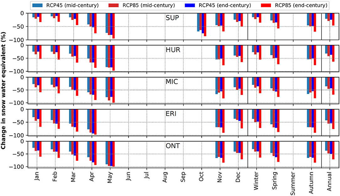
Figure 10. Percentage change in monthly, seasonal, and annual snow water equivalent (SWE) with respect to the baseline value for RCP 4.5 and RCP 8.5 scenarios in both mid- and end-century periods.
In the spring months (e.g., March and April), southern parts of the GL basin (e.g., Erie) are expected to lose almost 100% of its snowpack while northern parts (e.g., Superior) are expected to only retain only about 75% of the snowpack. For the winter season, during the end-century period using the RCP8.5 scenario, the Superior subdomain is expected to lose about 35% of the snowpack which increases to ~55% in Huron, ~60% in Michigan, ~70% in Erie, and ~65% in the Ontario subdomain (Figure 11).
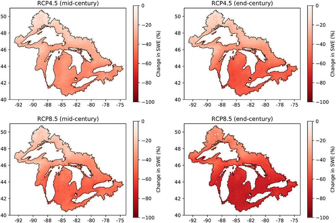
Figure 11. Percentage change in annual mean snow water equivalent (SWE) of GL basin for RCP 4.5 and RCP 8.5 scenarios in both mid- and end-century periods.
Actual Evapotranspiration
Projected increases in temperature of the GL basin will result in overall increase in annual AET (Figure 12). However, in the winter season, despite projected increases in temperature, slight decreases in AET are projected, especially during end-century period for RCP8.5 scenario. While it is evident that projected increases in temperature will increase potential evapotranspiration, the AET depends on several factors such as availability of soil moisture and vegetation type. Substantial projected decreases in snowpack (Figures 10, 11) and projected increases in high intensity rainfall (e.g., highest one-day precipitation, Supplementary Figure S7), would allow for more surface runoff and less infiltration, leading to lowered soil moisture conditions. Lowered soil moisture levels might be causing the decrease in AET in the winter season. Across all GL subdomains, projected increases in the summer AET are the highest, mainly driven by significant projected increases in summer temperature (Figure 9). Furthermore, substantial projected increases in summer day index (Supplementary Figure S10) would also result in projected increases in summer AET. Spring season AET also shows moderate increases across the GL basin. Autumn season AET in Ontario subdomain, unlike that observed in other subdomains, are projected to decrease in both future periods and for both emission scenarios. The overall autumn season AET decreases in the subdomain are mainly driven by projected decreases in AET in September.
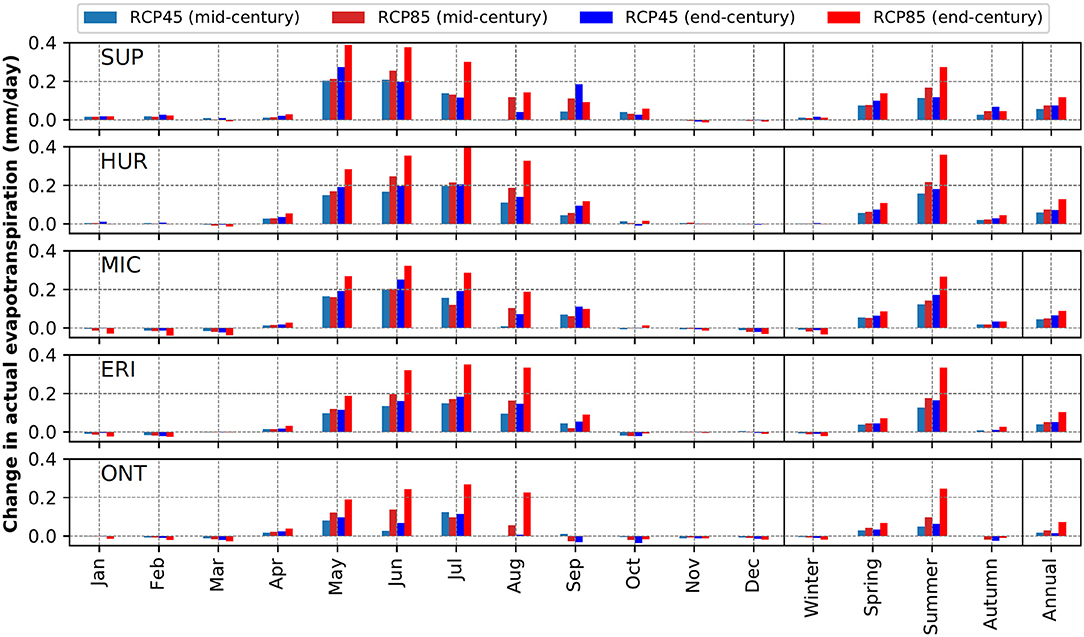
Figure 12. Absolute changes in monthly, seasonal, and annual actual evapotranspiration (AET) with respect to the baseline values for RCP 4.5 and RCP 8.5 scenarios in both mid- and end-century periods.
Spatially, the highest of increases (~15%) in annual AET are from water bodies such as man-made lake/reservoirs (Figure 13), this could be expected as AET from water bodies will be at the potential rate (PET). This is unlike the case in other landcover types such as agriculture or forest where AET may be limited by several factors such as availability of moisture in soil. Furthermore, it should be noted that we used Hargreaves method (Hargreaves and Samani, 1985) to estimate the rate of potential evapotranspiration. The use of such a simplified method for the estimation of AET from a dynamic system as the GL is subject to various forms of uncertainties and could reduce the accuracy of hydrological models. As stated in the Introduction section, the use of a hydrological model which utilizes temperature index (TI) methods such as the Hargreaves method in climate change impact studies has been questioned (Lofgren et al., 2011, 2013; Lofgren and Rouhana, 2016; Milly and Dunne, 2017). As such, projected increases (~15%) in annual AET around the Lake Nipigon (Figure 13) can thus be questioned. The use of an energy balance method to calculate PET would be preferred in such a lake (Finch and Calver, 2008), however, all the incoming and outgoing energy terms required to close the energy balance are not the outputs of the RCMs of the NA-CORDEX experiment. Hence, this should be considered as one of the limitations of the study.
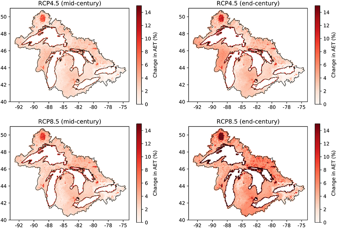
Figure 13. Percentage changes in annual mean actual evapotranspiration (AET) of GL basin for RCP 4.5 and RCP 8.5 scenarios both mid- and end-century periods.
Projected Changes in Runoff Into the Lakes
In the context of this study, the term runoff refers to the amount of water entering each lake through the stream network. This is the amount of water that comes from the land area (through overland flow, interflow, and baseflow) into the stream network, which is then routed downstream into the lakes. For operation purposes such as seasonal water level forecasting (Fry et al., 2020) or net basin supply (NBS) calculation (Do et al., 2020), runoff into each GL needs to be converted into equivalent effect on lake level. A ratio of land area to lake area of each GLs, as agreed by Coordinating Committee on Great Lakes basic hydraulic and hydrologic data, is used for this purpose (GLCC, 2021). As Lakes Huron and Michigan are hydrologically connected, runoff from land areas of both lakes (MHG) are aggregated and converted into their equivalent effect on lake level. While it is evident that the “runoff component of the NBS (or the effect of the runoff on lake level)” and the “runoff into the lakes from surrounding land areas” are two different quantities, for simplicity, we are referring the “runoff component of the NBS” as the “runoff” from hereafter.
Annual average runoff for Lakes Superior, Michigan-Huron, Erie and Ontario is projected to increase by 25–48, 18–40, 4–25, and 11–28%, respectively (Figure 14). Higher increases are projected for the RCP8.5 emission scenario and in the end-century period. It should be noted that both future annual precipitation and mean annual temperature (and as a result AET) are expected to increase in all subdomains (Supplementary Figures S5, S9). An equal increase in these factors may result in a net zero change in runoff. However, the overall increase in annual runoff is most likely a result of a greater change in the annual precipitation (Figure 5). On the other hand, accelerated melt of the snowpack can also lead to the overall increase. Amongst the seasons, the increase in runoff is projected to be the highest in the winter. For instance, in Superior subdomain, the winter runoff is expected to increase by 146%, which is significantly higher than the annual projected increase. The same trend is evident in other subdomains. spring season runoff is expected to have moderate increase due to already depleted snowpack, especially in southern subdomains (e.g., Ontario, 6–16%). The same behavior is evident in summer and autumn seasons across all subdomains except for Erie. In the Erie subdomain, runoff is expected to decrease in both future periods for the RCP4.5 emission scenario in summer and autumn. This is due to projected decrease in August and September precipitation in the subdomain (Supplementary Figure S5). At a monthly timescale, in the northern subdomains (e.g., Superior), the highest increases in runoff are observed in March (216%) while in southern subdomains (e.g., Ontario), the highest increases are, as expected, observed earlier (February, 111%). Availability of higher snowpack and higher increases in temperature in the northern subdomains (Figure S9) may have resulted in such significant increases, as compared to the southern subdomains.
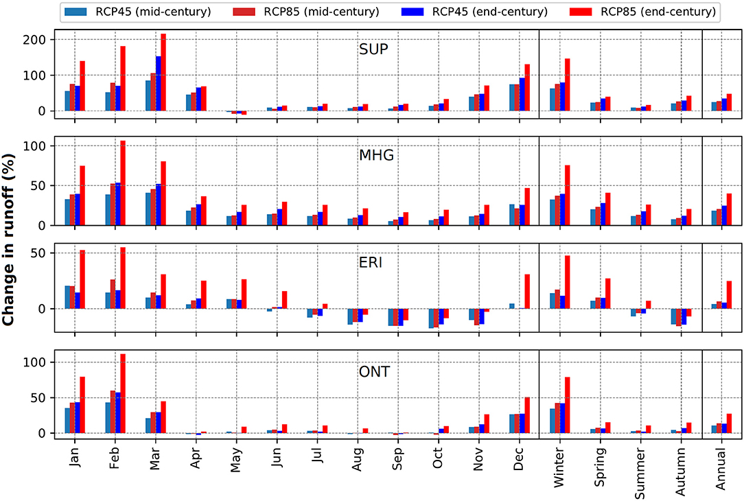
Figure 14. Change in monthly, seasonal, and annual runoff with respect to the baseline values for RCP4.5 and RCP8.5 scenarios in both mid- and end-century periods.
Probability exceedance plots of runoff (Supplementary Figure S11) further confirm the projected rise in the runoff and show the severity of changes: high (at 10% exceedance probability), mid (between 10 and 90% exceedance probability) and low (90% exceedance probability), following (USEPA, 2007) classification. In the Superior and Michigan-Huron subdomains, projected increases are evident for almost all exceedance probabilities. For instance, the ensemble mean of high runoff into Lake Superior is projected to increase up to 95 mm (in end-century period for RCP8.5 scenario) which is about 20% increase from its baseline value (80 mm). A similar increment (~30%, in end-century period for RCP8.5 scenario) is observed in runoff into Lake Michigan-Huron. In Lakes Erie and Ontario, projected changes in low runoff are minimal. In these southern subdomains, mid and high runoff are however projected to increase significantly. For instance, median runoff into Lakes Erie and Ontario are projected to increase by ~35 and ~20%, respectively.
Without analyzing the other components (over-lake precipitation and over-lake evaporation) of the net basin supply (NBS), it is impossible to determine whether future lake level will rise or drop. However, from the results of this study, it is quite evident that runoff component of the NBS is projected to increase in future. A recent analysis of the future changes of GL levels (Seglenieks and Temgoua, in review), indicated that under a changing climate more extreme highs and lows would be experienced, as well as a gradual increase in average lake levels. Such fluctuations in lake level may cause flooding and erosion along shoreline communities of the GL basin. Furthermore, key shoreline wetlands may experience detrimental effects of the projected fluctuations in water level of GLs, as also highlighted by Mortsch (1998).
Uncertainty Quantification
As there are 2 emission scenarios (ES) (RCP4.5 and RCP8.5), and 6 common regional climate models (RCM) between them, there were a total of 12 projections, of which 6 simulations and 2 simulations were considered at each stage of ES and RCM, respectively, to estimate their contribution to the total uncertainty. Relative contribution of ES and RCM into total uncertainty in future SWE, AET and runoff estimates are shown in Supplementary Tables S4A–C, respectively. It is quite evident that ES is by far the largest contributor to the total uncertainty. The contribution of ES to the total uncertainty is higher in end-century period as compared in mid-century period. As an example, in mid-century period, 68% of total uncertainty in SWE estimates is due to ES which increases to 85% in end-century period (Supplementary Table S4A). It indicates that the choice of the RCM is not so important, as far as the uncertainty in future projection of SWE is concerned. Rather, future SWE estimates will be highly dependent on the choice of an ES. While a similar trend is also observed for AET and runoff, the choice of RCM is still quite important for these variables as 35% (28%) and 36% (28%) of the total uncertainty is still contributed by RCM in mid-century (end-century) period. The use bias-corrected and high-resolution RCMs to derive future estimates of SWE, AET and runoff, may be one the reasons that the choice of a particular RCM may not constitute a significant source of uncertainty. A similar observation, ES being the largest contributor was also reported by Lee et al. (2017).
Summary and Conclusions
Freshwater resources of the Laurentian Great Lakes basin contribute significantly to the environment and economy of Canada and the United States. Sustainable management of the freshwater resources is thus very important. However, several stressors such as climate change will pose serious threats to these water resources in the future. Hence, an assessment of the impacts of climate change on land hydroclimatology is appropriate. This study uses a set of 36 simulations from 6 RCMs in historical (or baseline, 1951–2005) and two future (mid-century, 2035–2064 and end century, 2065–2094) periods, and for two emission scenarios (RCP4.5 and RCP8.5), to quantify trends and changes in land precipitation and temperature. As well as using the RCM projections as input to a calibrated and validated hydrological model, this study also assesses the impacts of climate change on snowpack, actual evapotranspiration and runoff into the lakes.
Results show that the GL land area will experience a wetter and warmer future with projected mean annual precipitation increases up to 15% and projected mean annual temperature increases up to 5°C. Seasonal (up to 25% increase in precipitation and up to 5.8°C increase in mean temperature) and monthly (up to 33% increase in precipitation and up to 6.0°C increase in mean temperature) changes are greater than the annual changes. Some scenarios even show projected decreases (~6% in August during mid-century period for RCP4.5 scenario) in summer precipitation. Projected increases in highest-one day precipitation and projected decreases in both wet days and consecutive wet days indicate occurrence of more future extreme precipitation in the GL basin. Similarly, results show that the GL basin will experience a lower number of ice days and a higher number of summer days in future.
The future snowpack in the GL basin is expected to decrease substantially (up to 76% in Erie subdomain). The highest decreases in snowpack are expected in the spring season, including up to 88% in the Erie subdomain for some scenarios. On the other hand, actual evapotranspiration is projected to increase in future with the highest projected increases in the summer (up to 0.4 mm/day). Results show consistent increases in runoff (up to 48%), with higher increases in the northern lakes (Superior and Michigan-Huron) than in the southern lakes (Erie and Ontario). By contrast, in the autumn season, some scenarios even show projected decreases (up to 16%) in runoff.
Uncertainty analysis showed that the use of different emission scenarios is the largest contributor to the total uncertainty and the choice of a particular RCM is not as important as far as the uncertainty in the future estimates of the snow water equivalent, actual evapotranspiration and runoff (to the lakes) are concerned.
A wetter and warmer future with more extreme precipitation, compounded by a substantial decrease in snowpack and an increase in actual evapotranspiration, will surely pose challenges to water resources managers and planners in the GL basin. Such a challenge due to competing forces in a future hydrological cycle of the GL basin was also corroborated by several other studies including Brown et al. (2011), Carter and Steinschneider (2018) and Gronewold and Rood (2019). Also of note, is that a majority of the most extreme effects are seen under the “business as usual” RCP 8.5 emission scenario particularly at the end of the century. There is of course more uncertainty in these results, as not only are they for many years in the future, but they will be highly dependent on future carbon emissions and thus how society adapts. Thus, these results should be seen as a guide to possible changes in the GL hydroclimate variables, but not as a forecast of the exact future conditions.
Amongst all the other GL basin (and surrounding region) historical climate change studies, it is hard to state whether the results of this study are more robust. We believe that the ensemble results that we obtained with the use of a set of high-resolution bias-corrected RCM forcings to a coupled hydrological model with explicit consideration of smaller lakes, evaluated not only for streamflow but also for other variables of interests (SWE and AET) are relatively reliable. The reader should also be aware of some studies (Lofgren et al., 2011, 2013; Lofgren and Rouhana, 2016; Milly and Dunne, 2017) questioning the use of a hydrological model utilizing temperature index (TI) method, rather than an energy-balance method, to project future changes in PET. The Hargreaves method (Hargreaves and Samani, 1985) is also a TI method that our hydrological model employs to calculate PET. However, the performance of the Hargreaves method as evident in some studies is encouraging. For example, of the four TI methods that Milly and Dunne, (2017) used to estimate the relative changes in future annual PET, the estimates when using the Hargreaves method were closest to the estimates of the energy-only method. Similarly, Xu and Singh (2001) evaluated the performance of seven TI methods in estimating evaporation at two climatological stations in Northwestern Ontario, Canada and recommended the use of the Hargreaves method. However, the use of an energy balance method in hydrological methods to estimate future changes in PET should be preferred if all the incoming and outgoing energy terms become outputs of high-resolution bias-corrected RCMs. Furthermore, this study quantifies the relative contribution of climate model and scenario uncertainties to the total uncertainty in considered hydrological variables which also provides a guidance to new studies.
We presume that better quantification of impacts of climate change on land-hydroclimatic variables will be helpful to understand the future conditions of the GL basin. This may also help formulate a coordinated effort to address the adverse effects of climate change in the basin.
Data Availability Statement
The raw data supporting the conclusions of this article will be made available by the authors, without undue reservation.
Author Contributions
Conceptualization and supervision: FS. Methodology and modeling: NS, FS, AT, and AD. Formal analysis and writing—review and editing: NS, FS, and AT. Data curation, writing—original draft preparation, and visualization: NS. All authors contributed to the article and approved the submitted version.
Conflict of Interest
The authors declare that the research was conducted in the absence of any commercial or financial relationships that could be construed as a potential conflict of interest.
Publisher's Note
All claims expressed in this article are solely those of the authors and do not necessarily represent those of their affiliated organizations, or those of the publisher, the editors and the reviewers. Any product that may be evaluated in this article, or claim that may be made by its manufacturer, is not guaranteed or endorsed by the publisher.
Acknowledgments
We would like to thank J. Mai of the University of Waterloo (UofW) for pre-processing spatial and meteorological data used in WATFLOOD model set-up, calibration, and validation. We would also like to thank E. Gaborit of Environment and Climate Change Canada (ECCC) for preparing separate input data for the five subdomains. We are also thankful to H. Shen of UofW who provided the lake and river routing product, incorporated in RAVEN for each subdomain. Many thanks to D. Princz of ECCC for helping to create a WATFLOOD executable with netCDF capabilities. We are also indebted to the RAVEN development team of UofW for providing a RAVEN-ro executable with netCDF capabilities.
Supplementary Material
The Supplementary Material for this article can be found online at: https://www.frontiersin.org/articles/10.3389/frwa.2022.801134/full#supplementary-material
References
Acharya, N., Shrivastava, N. A., Panigrahi, B. K., and Mohanty, U. C. (2014). Development of an artificial neural network based multi-model ensemble to estimate the northeast monsoon rainfall over south peninsular India: an application of extreme learning machine. Clim. Dyn. 43, 1303–1310. doi: 10.1007/s00382-013-1942-
Angel, J. R., and Kunkel, K. E. (2010). The response of Great Lakes water levels to future climate scenarios with an emphasis on Lake Michigan-Huron. J. Great Lakes Res. 36, 51–58. doi: 10.1016/j.jglr.2009.09.006
Argent, R. M. (2004). An overview of model integration for environmental applications—components, frameworks and semantics. Environ. Model. Softw.19. 219–234. doi: 10.1016/S1364-815200150-6
Bartolai, A. M., He, L., Hurst, A. E., Mortsch, L., Paehlke, R., and Scavia, D. (2015). Climate change as a driver of change in the Great Lakes St. Lawrence River Basin. J. Great Lakes Res. 41, 45–58. doi: 10.1016/j.jglr.2014.11.012
Basile, S. J., Rauscher, S. A., and Steiner, A. L. (2017). Projected precipitation changes within the Great Lakes and Western Lake Erie Basin: a multi-model analysis of intensity and seasonality. Int. J. Climatol. 37, 4864–4879. doi: 10.1002/joc.5128
Bingeman, A. K., Kouwen, N., and Soulis, E. D. (2006). Validation of the hydrological processes in a hydrological Model. J. Hydrol. Eng. 11, 451–463. doi: 10.1061/(ASCE)1084-0699(2006)11:5(451)
Bosch, N. S., Evans, M. A., Scavia, D., and Allan, J. D. (2014). Interacting effects of climate change and agricultural BMPs on nutrient runoff entering Lake Erie. J. Great Lakes Res. 40, 581–589. doi: 10.1016/j.jglr.2014.04.011
Briley, L. J., Rood, R. B., and Notaro, M. (2021). Large lakes in climate models: a Great Lakes case study on the usability of CMIP5. J. Great Lakes Res. 47, 405–418. doi: 10.1016/j.jglr.2021.01.010
Brown, C., Werick, W., Leger, W., and Fay, D. (2011). A Decision-Analytic approach to managing climate risks: application to the upper Great Lakes. JAWRA J. Am. Water Resour. Assoc. 47, 524–534. doi: 10.1111/j.1752-1688.2011.00552.x
Bukovsky, M. S., and Mearns, L. O. (2020). Regional climate change projections from NA-CORDEX and their relation to climate sensitivity. Clim. Change. 162, 645–665. doi: 10.1007/s10584-020-02835-x
Buttle, J., Muir, T., and Frain, J. (2004). Economic impacts of climate change on the canadian Great Lakes hydro electric power producers: a supply analysis. Can. Water Resour. J. Revue Canadienne Des Ressources Hydriques. 29, 89–110. doi: 10.4296/cwrj089
Byun, K., Chiu, C.-M., and Hamlet, A. F. (2019). Effects of 21st century climate change on seasonal flow regimes and hydrologic extremes over the Midwest and Great Lakes region of the US. Sci. Total Environ. 650, 1261–1277. doi: 10.1016/j.scitotenv.2018.09.063
Cannon, A. J. (2015). Selecting GCM Scenarios that span the range of changes in a multimodel ensemble: application to CMIP5 climate extremes indices. J. Clim. 28, 1260–1267. doi: 10.1175/JCLI-D-14-00636.1
Cannon, A. J. (2018). Multivariate quantile mapping bias correction: an N-dimensional probability density function transform for climate model simulations of multiple variables. Clim. Dyn. 50, 31–49. doi: 10.1007/s00382-017-3580-6
Carter, E., and Steinschneider, S. (2018). Hydroclimatological drivers of extreme floods on Lake Ontario. Warter Resour. Res. 54, 4461–4478. doi: 10.1029/2018WR022908
Chao, P. (1999). Great Lakes water resources: Climate change impact analysis with transient GCM scenarios. JAWRA J. AM. Water Resour.Assoc. 35, 1499–1507. doi: 10.1111/j.1752-1688.1999.tb04233.x
Chen, J., Chu, H., and Noormets, A. (2021). AmeriFlux BASE US-Oho Oak Openings, Ver. 7-5'. Berkeley: Lawrence Berkeley National Laboratory.
Cherkauer, K. A., and Sinha, T. (2010). Hydrologic impacts of projected future climate change in the Lake Michigan region. J. Great Lakes Res. 36, 33–50. doi: 10.1016/j.jglr.2009.11.012
Christensen, J., Kjellström, E., Giorgi, F., Lenderink, G., and Rummukainen, M. (2010). Weight assignment in regional climate models, Clim. Res. 44, 179–194. doi: 10.3354/cr00916
Cohen, S. J. (1986). Impacts of CO2-induced climatic change on water resources in the Great Lakes Basin. Clim. Change. 8, 135–153. doi: 10.1007/BF00139751
Collingsworth, P. D., Bunnell, D. B., Murray, M. W., Kao, Y.-C., Feiner, Z. S., Claramunt, R. M., et al. (2017). Climate change as a long-term stressor for the fisheries of the Laurentian Great Lakes of North America. Rev. Fish Biol. Fish. 27, 363–391. doi: 10.1007/s11160-017-9480-3
Cousino, L. K., Becker, R. H., and Zmijewski, K. A. (2015). Modeling the effects of climate change on water, sediment, and nutrient yields from the maumee river watershed. J. Hydrol: Reg. Stud. 4, 762–775. doi: 10.1016/j.ejrh.2015.06.017
Craig, J. R., Brown, G., Chlumsky, R., Jenkinson, R. W., Jost, G., Lee, K., et al. (2020). Flexible watershed simulation with the Raven hydrological modelling framework, Environ. Model. Softw. 129, 104728. doi: 10.1016/j.envsoft.2020.104728
Cranmer, A. J., Kouwen, N., and Mousavi, S.-F. (2001). Proving WATFLOOD: modelling the nonlinearities of hydrologic response to storm intensities. Can.J. Civ. Eng. 28, 837–855. doi: 10.1139/l01-049
Croley, T. E. (1990). Laurentian Great Lakes double-CO2 climate change hydrological impacts. Clim. Change. 17, 27–47. doi: 10.1007/BF00148999
Crosbie, R. S., Dawes, W. R., Charles, S. P., Mpelasoka, F. S., Aryal, S., Barron, O., et al. (2011). Differences in future recharge estimates due to GCMs, downscaling methods and hydrological models. Geophys. Res. Lett. 38, 1–5. doi: 10.1029/2011GL047657
De Scheer, G., Therrien, R., Refsgaard, J. C., and Hansen, A. L. (2015). Simulating coupled surface and subsurface water flow in a tile-drained agricultural catchment. J. Hydrol. 521, 374–388. doi: 10.1016/j.jhydrol.2014.12.035
Do, H. X., Smith, J. P., Fry, L. M., and Gronewold, A. D. (2020). Seventy-year long record of monthly water balance estimates for Earth's largest lake system. Sci. Data. 7, 276. doi: 10.1038/s41597-020-00613-z
ELPC (2019). An Assessment of the Impacts of Climate Change on the Great Lakes. Chicago, USA: Environmental Law and Policy Center (ELPC).
Fahad, S., Bajwa, A. A., Nazir, U., Anjum, S. A., Farooq, A., Zohaib, A., et al. (2017). Crop Production under drought and heat stress: plant rsponses and management options. Fron. Plant. Sci. 8, 1147. doi: 10.3389/fpls.2017.01147
Finch, J., and Calver, A. (2008). Methods for the Quantification of Evaporation from Lakes. Wallingford, UK: CEH Wallingford.
Fluxnet Canada, T. (2016). FLUXNET Canada Research Network - Canadian Carbon Program Data Collection, 1993-2014. Oak Ridge: Oak Ridge National Laboratory Distributed Active Archive Center
Fry, L. M., A s, D., and Gronewold, A. D. (2020). Operational seasonal water suly and water level forecasting for the laurentian Great Lakes. J. Water Resour. Plann. Manag. 146, 04020072. doi: 10.1061/(ASCE)WR.1943-5452.0001214
Gasset, N., Fortin, V., Dimitrijevic, M., Carrera, M., Bilodeau, B., Muncaster, R., et al. (2021). A 10 km North American precipitation and land-surface reanalysis based on the GEM atmospheric model. Hydrol. Earth Syst. Sci. 25, 4917–4945. doi: 10.5194/hess-25-4917-2021
Gay, C., and Estrada, F. (2010). Objective probabilities about future climate are a matter of opinion. Clim. Change. 99, 27–46. doi: 10.1007/s10584-009-9681-4
GLCC (2021). Great Lakes Coordinating Committee. Available online at: www.greatlakescc.org/wp36/ (accessed December 2021).
Gough, C., Bohrer, B., and Curtis, P. (2021). AmeriFlux BASE US-UMB Univ. of Mich. Biological Station, Ver. 17-5.
Grady, K. A., Chen, L., and Ford, T. W. (2021). Projected changes to spring and summer precipitation in the Midwestern United States. Front. Water. 3, 1–16. doi: 10.3389/frwa.2021.780333
Gronewold, A. D., and Rood, R. B. (2019). Recent water level changes across Earth's largest lake system and implications for future variability. J. Great Lakes Res. 45, 1–3. doi: 10.1016/j.jglr.2018.10.012
Gupta, H. V., Kling, H., Yilmaz, K. K., and Martinez, G. F. (2009). Decomposition of the mean squared error and NSE performance criteria: implications for improving hydrological modelling J. Hydrol. 377, 80–91. doi: 10.1016/j.jhydrol.2009.08.003
Hall, K. R., Herbert, M. E., Sowa, S. P., Mysorekar, S., Woznicki, S. A., Nejadhashemi, P. A., et al. (2017). Reducing current and future risks: using climate change scenarios to test an agricultural conservation framework. J. Great Lakes Res. 43, 59–68. doi: 10.1016/j.jglr.2016.11.005
Han, M., Mai, J., Tolson, B. A., Craig, J. R., Gaborit, É., Liu, H., et al. (2020). Subwatershed-based lake and river routing products for hydrologic and land surface models a lied over Canada. Can. Water Resour. J. Revue canadienne des ressources hydriques. 45, 237–251. doi: 10.1080/07011784.2020.1772116
Hargreaves, G. H., and Samani, Z. A. (1985). Reference crop evapotranspiration from temperature. Lied Eng. Agric. 1, 96–99. doi: 10.13031/2013.26773
Hartmann, H. C. (1990). Climate change impacts on Laurentian Great Lakes levels. Clim. Change. 17, 49–67. doi: 10.1007/BF00149000
Hawkins, E., and Sutton, R. (2009). The Potential to narrow uncertainty in regional climate predictions. Bull. Am. Meteor. Soc. 90, 1095–1107. doi: 10.1175/2009BAMS2607.1
Hayhoe, K., VanDorn, J., Croley, T., Schlegal, N., and Wuebbles, D. (2010). Regional climate change projections for Chicago and the US Great Lakes. J. Great Lakes Res. 36, 7–21. doi: 10.1016/j.jglr.2010.03.012
Hellmann, J. J., Nadelhoffer, K. J., Iverson, L. R., Ziska, L. H., Matthews, S. N., Myers, P., et al. (2010). Climate change impacts on terrestrial ecosystems in metropolitan Chicago and its surrounding, multi-state region. J. Great Lakes Res. 36, 74–85. doi: 10.1016/j.jglr.2009.12.001
Homer, C., Colditz, R. R., Latifovic, R., Llamas, R. M., Pouliot, D., Danielson, P., et al. (2017). Developing a New North American Land Cover Product at 30m Resolution: Methods, Results and Future Plans. Orleans: American Geophysical Union, Fall Meeting.
Hostetler, S. W., Bates, G. T., and Giorgi, F. (1993). Interactive coupling of a lake thermal model with a regional climate model. J. Geophys. Res. Atmos. 98(D3), 5045–5057. doi: 10.1029/92JD02843
IJC (2021). International Joint Commission. Available online at: https://ijc.org/en (accessed: September 2021).
IPCC (2007). Climate Change 2007: Impacts, Adaptation and Vulnerability. Contribution of Working Group II to the Fourth Assessment Report of the Intergovernmental Panel on Climate Change. Cambridge, U.K.: Cambridge University Press. p. 976.
IPCC (2014). Climate Change 2014: Synthesis Report. Contribution of Working Groups I, II and III to the Fifth Assessment Report of the Intergovernmental Panel on Climate Change. Cambridge: IPCC.
IPCC (2021). “Summary for Policymakers”, in: Climate Change 2021: The Physical Science Basis. Contribution of Working Group I to the Sixth Assessment Report of the Intergovernmental Panel on Climate Change, Masson-Delmotte, V., Zhai, P., Pirani, A., Connors, S.L., Péan, C., and Berger, S., (eds). Cambridge University Press. Geneva: Intergovernmental Panel on Climate Change.
Kling, G., Hayhoe, K., Johnson, L., Magnuson, J., Polassky, S., Robinson, S., et al. (2003). Confronting Climate Change in the Great Lakes Region: Impacts on Our Communities and Ecosystems.
Kouwen, N. (1986). WATFLOOD/CHARM Canadian Hydrological And Routing Model. Waterloo, Ontario. Canada: Department of Civil Engineering University of Waterloo.
Kouwen, N. (1988). WATFLOOD: a micro-computer based flood forecasting system based on real-time weather radar. Can. Water Resour. J. 13, 62–77. doi: 10.4296/cwrj1301062
Kouwen, N., Danard, M., Bingeman, A., Luo, W., Seglenieks, F., and Soulis, E. (2005). Case Study: watershed modeling with distributed weather model data. J. Hydrol. Engi. 10, 23–38. doi: 10.1061/(ASCE)1084-0699(2005)10:1
Kouwen, N., Soulis, E. D., Pietroniro, A., Donald, J., and Harrington, R. A. (1993). Grouped response units for distributed hydrologic modeling. J. Water Resour. Plann. Manag. 119, 289–305. doi: 10.1061/(ASCE)0733-9496(1993)119:3(289)
Krysanova, V., Donnelly, C., Gelfan, A., Gerten, D., Arheimer, B., Hattermann, F., et al. (2018). How the performance of hydrological models relates to credibility of projections under climate change Hydrol. Sci. J. 63. 696–720, doi: 10.1080/02626667.2018.1446214
Kunkel, K. E., Ensor, L., Palecki, M., Easterling, D., Robinson, D., Hubbard, K. G., et al. (2009). A new look at lake-effect snowfall trends in the Laurentian Great Lakes using a temporally homogeneous data set. J. Great Lakes Res. 35, 23–29. doi: 10.1016/j.jglr.2008.11.003
Kutzbach, J., Williams, J., and Vavrus, S. (2005). Simulated 21st century changes in regional water balance of the Great Lakes region and links to changes in global temperature and poleward moisture transport Geophys. Res. Lett. 32, 1–5. doi: 10.1029/2005GL023506
Larson, G., and Schaetzl, R. (2001). Origin and evolution of the Great Lakes. J. Great Lakes Res. 27. 518–546. doi: 10.1016/S0380-133070665-X
Lee, J.-K., Kim, Y.-O., and Kim, Y. (2017). A new uncertainty analysis in the climate change impact assessment. Int.J. Climatol. 37, 3837–3846. doi: 10.1002/joc.4957
Lehner, B., Verdin, K. L., and Jarvis, A. (2008). New global hydrography derived from spaceborne elevation data. Eos. Trans, Am. Geophys. Union. 89, 93–94. doi: 10.1029/2008EO100001
Lofgren, B. M., Gronewold, A. D., Acciaioli, A., Cherry, J., Steiner, A., and Watkins, D. (2013). Methodological a roaches to projecting the hydrologic impacts of climate change. E I. 17, 1–19. doi: 10.1175/2013EI000532.1
Lofgren, B. M., Hunter, T. S., and Wilbarger, J. (2011). Effects of using air temperature as a proxy for potential evapotranspiration in climate change scenarios of Great Lakes basin hydrology. J. Great Lakes Res. 37, 744–752. doi: 10.1016/j.jglr.2011.09.006
Lofgren, B. M., Quinn, F. H., Clites, A. H., Assel, R. A., Eberhardt, A. J., and Luukkonen, C. L. (2002). Evaluation of potential impacts on great lakes water resources based on climate scenarios of two GCMs. J. Great Lakes Res. 28, 537–554. doi: 10.1016/S0380-133070604-7
Lofgren, B. M., and Rouhana, J. (2016). Physically Plausible methods for projecting changes in great lakes water levels under cclimate change scenarios. J. Hydrometeorol. 17, 2209–2223. doi: 10.1175/JHM-D-15-0220.1
Lutz, A. F., ter Maat, H. W., Biemans, H., Shrestha, A. B., Wester, P., and Immerzeel, W. W. (2016). Selecting representative climate models for climate change impact studies: an advanced envelope-based selection approach. Int. J. Climatol. 36, 3988–4005. doi: 10.1002/joc.4608
Mackay, M., and Seglenieks, F. (2012). On the simulation of Laurentian Great Lakes water levels under projections of global climate change. Clim. Change 117, 55–67. doi: 10.1007/s10584-012-0560-z
Mai, J., Shen, H., Tolson, B. A., Gaborit, É., Arsenault, R., Craig, J. R., et al. (2022). The great lakes runoff intercomparison project phase 4: the great lakes (GRIP-GL). Hydrol. Earth Syst. Sci. Discussion. 2022, 1–54, doi: 10.5194/hess-2022-113
Mai, J., Tolson Bryan, A., Shen, H., Gaborit, É., Fortin, V., Gasset, N., et al. (2021). Great lakes runoff intercomparison project phase 3: lake Erie (GRIP-E). J. Hydrol. Engi. 26, 05021020. doi: 10.1061/(ASCE)HE.1943-5584.0002097
Mailhot, E., Music, B., Nadeau, D. F., Frigon, A., and Turcotte, R. (2019). Assessment of the laurentian great lakes' hydrological conditions in a changing climate. Clim. Change. 157, 243–259. doi: 10.1007/s10584-019-02530-6
Mann, H. B. (1945). Nonparametric tests against trend. Econometrica. 13, 245–259. doi: 10.2307/1907187
Marchand, D., Sanderson, M., Howe, D., and Alpaugh, C. (1988). Climatic change and great lakes levels the impact on shi ing. Clim. Change. 12, 107–133. doi: 10.1007/BF00138935
Marks, D., Kimball, J., Tingey, D., and Link, T. (1998). The sensitivity of snowmelt processes to climate conditions and forest cover during rain-on-snow: a case study of the 1996 Pacific Northwest flood. Hydrol. Process. 12, 1569–1587. doi: 10.1002/(SICI)1099-1085(199808/09)12:10/11<1569::AID-HYP682>3.0.CO;2-L
Matott, L. (2017). OSTRICH: An Optimization Software Tool, Documentation and User's Guide, Version 17.12.19. University at Buffalo Center for Computational Research. Geneva: Intergovernmental Panel on Climate Change.
Mearns, L. O., McGinnis, S., Korytina, D., Arritt, R., Biner, S., and Bukovsky, M. (2017). 'The NA-CORDEX Dataset, Version 1.0.
Meehl, G. A., Covey, C., Delworth, T., Latif, M., McAvaney, B., Mitchell, J. F. B., et al. (2007). THE WCRP CMIP3 multimodel dataset: a New era in climate change research. Bull. Am. Meteorol. Soc. 88, 1383–1394. doi: 10.1175/BAMS-88-9-1383
Millerd, F. (2005). The economic impact of climate change on canadian commercial navigation on the Great Lake. Can Water Resour. J. Revue canadienne des ressources hydriques. 30, 269–280. doi: 10.4296/cwrj3004269
Milly, P. C. D., and Dunne, K. A. (2017). A hydrologic drying Bias in water-resource impact analyses of aanthropogenic climate change. JAWRA J. Am. Water Resour.Assoc. 53, 822–838. doi: 10.1111/1752-1688.12538
Mironov, D., Kourzeneva, E., Ritter, B., and Schneider, N. (2009). Implementation of the lake parameterisation scheme FLake into numerical weather prediction model COSMO', Boreal Environ. Res. 15. Available online at: http://www.borenv.net/BER/archive/pdfs/ber15/ber15-097.pdf
Mortsch, L., Hengeveld, H., Lister, M., Wenger, L., Lofgren, B., Quinn, F., et al. (2000). Climate Change Impacts on the Hydrology of the Great Lakes-St. Lawrence System. Can. Water Resour. J. 25,153–179. doi: 10.4296/cwrj2502153
Mortsch, L. D. (1998). Assessing the impact of climate change on the great lakes shoreline wetlands. Clim. Change. 40. 391–416. doi: 10.1023/A:1005445709728
MPM (2022). Great Lakes History: A General View. Milwaukee Public Museum (MPM). Available online at: https://www.mpm.edu/content/wirp/ICW-21 (accessed May 9, 2021).
Music, B., Frigon, A., Lofgren, B., Turcotte, R., and Cyr, J.-F. (2015). Present and future Laurentian Great Lakes hydroclimatic conditions as simulated by regional climate models with an emphasis on lake Michigan-Huron. Clim. Change. 130, 603–618. doi: 10.1007/s10584-015-1348-8
Musselman, K. N., Clark, M. P., Liu, C., Ikeda, K., and Rasmussen, R. (2017). Slower snowmelt in a warmer world. Nat. Clim. Chang. 7, 214–219. doi: 10.1038/nclimate3225
Musselman, K. N., Lehner, F., Ikeda, K., Clark, M. P., Prein, A. F., Liu, C., et al. (2018). Projected increases and shifts in rain-on-snow flood risk over western North America. Nat. Climat. Chang. 8, 808–812. doi: 10.1038/s41558-018-0236-4
NA-CORDEX (2022). Major Characteristics of Rregional Climate Models used in NA-CORDEX. Available online at: https://na-cordex.org/rcm-characteristics.html. (accessed on May 9, 2022).
Neitsch, S. L., Arnold, J. G., Kiniry, J. R., and Williams, J. R. (2011). Soil and Water Assessment Tool Theoretical Documentation, Version 2009: Grassland,Soil and Water Research Laboratory-Agricultural Research Service. Temple: Texas A&M AgriLife Blackland Research & Extension Center.
Notaro, M., Bennington, V., and Lofgren, B. (2015). Dynamical downscaling–based projections of Great Lakes water levels, J. Clim. 28, 9721–9745. doi: 10.1175/JCLI-D-14-00847.1
Notaro, M., Holman, K., Zarrin, A., Fluck, E., Vavrus, S., and Bennington, V. (2013). Influence of the Laurentian Great Lakes on regional climat. J. Clim. 26, 789–804. doi: 10.1175/JCLI-D-12-00140.1
Ohn, I., Seo, S. B., Kim, S., Kim, Y.-O., and Kim, Y. (2020). Uncertainty decomposition in climate-change impact assessments: a bayesian perspective. Comm. Stat. Alication.Methods. 27, 109–128. doi: 10.29220/CSAM.2020.27.1.109
Pomeroy, J. W., Stewart, R. E., and Whitfield, P. H. (2016). The 2013 flood event in the south askatchewan and Elk river basins: Causes, assessment and damages. Can. Water Resour. Journal / Revue canadienne des ressources hydriques, 41, 105–117. doi: 10.1080/07011784.2015.1089190
Rahman, M., Bolisetti, T., and Balachandar, R. (2010). Effect of climate Change on low-flow conditions in the ruscom river watershed, ontario. Trans. ASABE. 53, 1521. doi: 10.13031/2013.34904
Requena, A. I., Nguyen, T.-H., Burn, D. H., Coulibaly, P., and Nguyen, V.-T.-V. (2021). 'A temporal downscaling a roach for sub-daily gridded extreme rainfall intensity estimation under climate change. J. Hydrol: Reg. Stud. 35, 100811. doi: 10.1016/j.ejrh.2021.100811
Schwartz, R. C., Deadman, P. J., Scott, D. J., and Mortsch, L. D. (2004). Modelling the impacts of water level changes on a Great Lakes community. JAWRA J. Am. water Resour.Assoc. 40, 647–662. doi: 10.1111/j.1752-1688.2004.tb04450.x
Seglenieks, F. R., Soulis, E. D., and Kouwen, N. (2004). Closing the Water Balance on the Mackenzie River using the models WATFLOOD and WATCLASS. American Geophysical Union. Spring Meeting 2004.
Shrestha, N. K., Seflenieks, F., Shen, H., and Mai, J. (2021). SWAT-RAVEN Coupled Models for Enhanced Streamflow Simulation over the great lakes region. 64th Annual Conference on Great Lakes Research, Michigan Technological University.
Smith, J. B. (1991). The potential impacts of climate change on the great lakes. Bul. Amer. Meteor. Soc. 72, 21–28. doi: 10.1175/1520-0477(1991)072<0021:TPIOCC>2.0.CO;2
Smith, L. A. (2002). 'What might we learn from climate forecasts?. Proc. Nat. Acad. Sci. 99, 487–2492. doi: 10.1073/pnas.012580599
Sobota, I., Weckwerth, P., and Grajewski, T. (2020). Rain-On-Snow (ROS) events and their relations to snowpack and ice layer changes on small glaciers in Svalbard, the higha. J. Hydrol. 590, 125279. doi: 10.1016/j.jhydrol.2020.125279
Taylor, K. E., Stouffer, R. J., and Meehl, G. A. (2011). An overview of CMIP5 and the experiment design, Bull. Amer. Meteorol. Soc. 93, 485–498. doi: 10.1175/BAMS-D-11-00094.1
Thornthwaite, C. W. (1948).An a roach toward a rational classification of climate. Geogr. Rev. 38. 55–94, doi: 10.2307/210739
Thornton, M. M., Shrestha, R., Wei, Y., Thornton, P. E., Kao, S., and Wilson, B. E. (2020). Daymet: Daily Surface Weather Data on a 1-km Grid for North America, Version 4. Oak Ridge: Oak Ridge National Laboratory Distributed Active Archive Center.
Tolson, B. A., and Shoemaker, C. A. (2007). Dynamically dimensioned search algorithm for computationally efficient watershed model calibration, Water Resour. Res. 43, 1–16. doi: 10.1029/2005WR004723
USEPA (2007). An A Roach for Using Load Duration Curves in the Development of TMDLs. Washington DC: US Environmental Protection AgencyEPA 841-B-07-006.
USEPA (2021). Facts and Figures about the Great Lakes: United States Environmental Protection Agency. Available online at: https://www.epa.gov/greatlakes/facts-and-figures-about-great-lakes
USEPA-GoC (1995). The great-lakes—An Environmental Atlas and Resource Book: US Environmental Protection Agency and Government of Canada, 1–51.
Valiante, M. (2008). “Management of the North American Great Lakes”, in Management of Transboundary Rivers and Lakes, Varis, O., Biswas, A.K. and Tortajada, C (eds). Berlin, Heidelberg: Springer Berlin Heidelberg. p. 245–267. doi: 10.1007/978-3-540-74928-8_10
VanDeWeghe, A., Lin, V., Jayaram, J., and Gronewold, A. D. (2022). Changes in large lake water level dynamics in response to climate change, Front. Water 4. doi: 10.3389/frwa.2022.805143
Verma, S., Bhattarai, R., Bosch Nathan, S., Cooke Richard, C., Kalita Prasanta, K., and Markus, M. (2015). Climate change impacts on flow, sediment and nutrient export in a great lakes watershed using SWAT. CLEAN .Soil. Air. Water. 43, 1464–1474. doi: 10.1002/clen.201400724
Vionnet, V., Mortimer, C., Brady, M., Arnal, L., and Brown, R. (2021). 'Canadian historical Snow Water Equivalent dataset (CanSWE, 1928–2020). Earth Syst. Sci. Data. 13, 4603–4619. doi: 10.5194/essd-13-4603-2021
Wallace, C. W., Flanagan, D. C., and Engel, B. A. (2017). Quantifying the effects of future climate conditions on runoff, sediment, and chemical losses at different watershed sizes. Trans. ASABE. 60, 915–929. doi: 10.13031/trans.12094
Wang, X., Huang, G., and Baetz, B. W. (2016). Dynamically-downscaled probabilistic projections of precipitation changes: a Canadian case study. Environ. Res. 148, 86–101. doi: 10.1016/j.envres.2016.03.019
Whorley, D. (2020). “From IWC to WT Canada-US Institution Building, 1902–1909”, in The First Century of the International Joint Commission, Macfarlane, D., and Clamen, M., (eds). Calgary: University of Calgary Press. p. 35–70. doi: 10.2307/j.ctvvb7kmv.7
Winkler, J. A., Arritt, R. W., and Pryor, S. C. (2012). “Climate Projections for the Midwest: Availability, Interpretation and Synthesis”, in U.S. National Climate Assessment Midwest Technical Input Report, Winkler, J., Andresen, J., Hatfield, J., Bidwell, D., and Brown, D,. (eds) Ann Arbor: Great Lakes Integrated Sciences and Assessment (GLISA) Center.
Wright, D. M., Posselt, D. J., and Steiner, A. L. (2013). Sensitivity of lake-effect snowfall to lake ice cover and temperature in the great lakes region. Mon. Weather Rev.141, 670–689. doi: 10.1175/MWR-D-12-00038.1
Wuebbles, D. J., Hayhoe, K., and Parzen, J. (2010). Introduction: assessing the effects of climate change on Chicago and the Great Lakes. J. Great Lakes Res. 36, 1–6. doi: 10.1016/j.jglr.2009.09.009
Xu, C. Y., and Singh, V. P. (2001). Evaluation and generalization of temperature-based methods for calculating evaporation. Hydrol. Process. 15, 305–319. doi: 10.1002/hyp.119
Xu, X., Wang, Y.-C., Kalcic, M., Muenich, R. L., Yang, Y. C. E., and Scavia, D. (2019). Evaluating the impact of climate change on fluvial flood risk in a mixed-use watershed. Environ. Modell. Softw.122, 104031. doi: 10.1016/j.envsoft.2017.07.013
Yassin, F., Razavi, S., Elshamy, M., Davison, B., Sapriza-Azuri, G., and Wheater, H. (2019). Representation and improved parameterization of reservoir operation in hydrological and land-surface models. Hydrol. Earth Syst. Sci. 23, 3735–3764. doi: 10.5194/hess-23-3735-2019
Keywords: Laurentian Great Lakes, climate change, land hydroclimatology, water resources management, RCM
Citation: Shrestha NK, Seglenieks F, Temgoua AGT and Dehghan A (2022) The Impacts of Climate Change on Land Hydroclimatology of the Laurentian Great Lakes Basin. Front. Water 4:801134. doi: 10.3389/frwa.2022.801134
Received: 24 October 2021; Accepted: 17 June 2022;
Published: 11 July 2022.
Edited by:
Galina Guentchev, Met Office, United KingdomReviewed by:
Fuad Yassin, University of Saskatchewan, CanadaAndrew Gronewold, University of Michigan, United States
Copyright © 2022 Shrestha, Seglenieks, Temgoua and Dehghan. This is an open-access article distributed under the terms of the Creative Commons Attribution License (CC BY). The use, distribution or reproduction in other forums is permitted, provided the original author(s) and the copyright owner(s) are credited and that the original publication in this journal is cited, in accordance with accepted academic practice. No use, distribution or reproduction is permitted which does not comply with these terms.
*Correspondence: Frank Seglenieks, ZnJhbmsuc2VnbGVuaWVrc0BlYy5nYy5jYQ==