Verification of PCSWMM's LID processes and their scalability over time and space

Introduction: This paper explores the scalability of PCSWMM's Low Impact Development (LID) modeling tools within the urban stormwater computer model.

Methods: The scalability is assessed for a variety of spatial and temporal scales and for event (50-year return storm) and continuous inputs (daily rainfall for an 11 month period), and with a focus on bioretention cells. The model is calibrated for a moderate to large scale, semi-urban watershed on Vancouver Island, British Columbia, Canada. Sensitivity analysis and specialized metrics are used to verify internal model processes at a variety of scales.

Results: With regard to spatial scaling, changes in flow path length and slope derived from Digital Elevation Models were the most impactful spatial information when modeling flood event and the model's surface layer was the dominant contributor to peak flowrate and volume mitigation by the bioretention cell. However, when modeling the continuous rainfall inputs, storage layer related parameters dominated model outputs. Aside from the soil layer's depth, soil layer parameters such as hydraulic conductivity, showed negligible influence on response to time series rainfall. Parameters that are kept static by the model such as vegetation cover, hydraulic conductivity and storage void ratio (but are naturally dynamic), were tested for their impact on response if allowed to change seasonally or with excessive loading. Runoff coefficients were greatly impacted by storage layer parameter dynamics with very little impact from vegetation. For event simulations, the berm height in the surface layer was the dominant player in reducing peak flow as well as total volume. An analysis to help illustrate sensitivity across spatial scales is proposed.

Discussion: The Spatial Dynamic Sensitivity Analysis shows that parameter sensitivity changes dynamically as LID implementation percentage changes. In particular, the clogging factor, which is a parameter associated with the storage layer, was highly influential for time series rainfall analysis. The LID model concepts in PCSWM seem appropriate for events because the surface layer dominates the response for very large storms. For smaller storms, continuous time series, and larger spatial scales, the model could be revised to better represent soil layer dynamics and vegetation cover, which were both currently inconsequential to the model's output.

Introduction

Urbanization leads to increasing stormwater runoff and flooding (Ahiablame and Shakya, 2016; Shaneyfelt et al., 2021) as well as degrading the quality of receiving waters. Low Impact Development (LID) technologies are systems or practices that use or mimic natural processes to mitigate the deleterious effects of the increase in imperviousness arising from urbanization (Environmental Protection Agency, 2012; Paule-Mercado et al., 2017). LIDs include green roofs, bioretention cells, permeable pavements, cisterns, etc. (Golden and Hoghooghi, 2018), and provide a myriad of hydrological and environmental benefits, including runoff volume and peak reduction, groundwater recharge by increasing stormwater infiltration into the native soil, water quality improvements, heat-island effect mitigation (Xie et al., 2019), reduce soil sealing effects (Rodríguez-Rojas and Grindlay Moreno, 2022), etc. Having evolved in urban areas, LIDs are typically implemented at small scales. At these scales, LIDs have been demonstrated as effective tools through laboratory and field studies as well as in practice (Stovin et al., 2012; Palla and Gnecco, 2015; Gülbaz and Kazezyilmaz-Alhan, 2017b; Piro et al., 2019). They are shown to effectively reduce, mitigate, and prevent hydrological and meteorological risks at small scales or plot scales (Jiang et al., 2015; Palla and Gnecco, 2015; Herrera-Gomez et al., 2017; Liu et al., 2017; Seo et al., 2017; Bai et al., 2018). However, when evaluating the effectiveness of the LID, researchers often separate the LID from the hydrological water cycle system and considered it a separate component. This effectively ignores the interconnectedness between components of the hydrological process and flow transformation in the upstream and downstream zones (Nika et al., 2020), thereby reducing the ability to scale-up these infrastructure to larger, catchment scales. Statistical analysis shows, that where LID implementation area is greater than 5% of the drainage area, there is only a slight improvement in catchment water quantity and quality mitigation. This improvement may increase with the area where LIDs are implemented (Pennino et al., 2016) and naturally, the size of LID implementation on a large scale will be the dominant factor in evaluating LID performance. In the literature, large scale LID simulations seem to be primarily used for flood control (Lilburne and Tarantola, 2009; Carvalho et al., 2019) and few studies have focused on evaluating the outcomes of LIDs at larger scales (D'Ambrosio et al., 2022). In addition, studies have shown that the performance of LIDs varies greatly with rainfall distribution, and LIDs tend to perform better in response to rainfall patterns that are of low rainfall intensity, frequent and of short-duration (Peng et al., 2019), which tend not to result in flooding. Despite this, there is interest in scaling up LID implementation to larger, or catchment scales, instead of just being relegated to small-scale, urban areas (Golden and Hoghooghi, 2018). To do this successfully means that the interconnection between the LID and the rest of the catchment's hydrological components must be understood at these larger scales. Currently, because LIDs are studied at small spatial scales, there is a lack of design guidelines for large scale LIDs in watersheds, thus, preventing implementation at these larger scales (Martin-Mikle et al., 2015). The complexity associated with large scales and data availability issues can also limit the implementation at larger scales. The natural complexity of the interconnections in catchment hydrological components leads to higher uncertainties in hydrological model output. Thus, any LID model that ignores these interconnections would lead to a reduction in accuracy in predictions of LID function (Kaykhosravi et al., 2018).

LID design, construction and operation is often conducted through computer models that can simulate LID function. PCSWMM is a very popular urban stormwater model that has incorporated LID concepts to model the urban hydrology of catchments that contain such infrastructure. It uses quasi-physically based representations of hydrological processes in catchments with pervious areas, impervious areas, and LIDs. Like any conceptual, hydrological computer model, the water balance and dynamics are modeled with calibrated or default parameters based on the literature, user experience, or developer recommendations. These parameters can dramatically impact simulation results (Carvalho et al., 2019) depending on the mathematical representation of hydrological processes. PCSWMM's representation of LIDs has given rise to numerous applications (Sakshi and Singh, 2016; Bond et al., 2021; Jeffers et al., 2022) in the literature with calibrations and validations on a wide variety of catchments. However, PCSWMM's representation of LID processes has yet to be verified.

Verification of a model, unlike validation, is the process by which a model's concepts are assessed for representing reality within the bounds of uncertainty. To verify PCSWMM's representation of LIDs installed in moderate to large scale catchments, an analysis of the LID concepts/equations is required. This analysis must assess the reliability and degree of consistency in the LID mathematical representation for simulating actual observations for a wide range of spatial and dynamic heterogeneity. It must also assess the model's ability to realistically represent the various components of the catchments' hydrological water balance over space and time. Currently, five different LID tools are modeled by PCSWMM and each is conceptualized as a combination of vertical layers (Ahiablame and Shakya, 2016). The tools range from bioretention cells, rain gardens (unlined bioretention cells that drain to natural surrounding soils), green roofs, permeable pavements and others. There are large differences in these types of LIDS but fundamentally, PCSWMM models the first four types as layers in which water flows into adjacent lower layers. Thus, three layers are used to represent the LID: a surface layer (bioretention cell, green roof) sitting above a soil layer (or pavement layer in the case of permeable pavements) that drains into a storage layer beneath the soil layer. Layer characteristics and model equations depend on the type of surface, pavement if any, soil type and subsurface storage capacity. PCSWMM provides single- and multi-objective optimization techniques for calibrating the parameters associated with each layer in the model (Tobio et al., 2015).

A useful method for verifying simulated processes in hydrological models is a sensitivity analysis (SA) (Pfannerstill et al., 2015). This method determines the uncertainty in model output given different sources of uncertainty in the inputs (Saltelli et al., 2004) and has been widely used in hydrological model research (Wagener et al., 2003; Reusser et al., 2009). Temporal Dynamics of Parameter Sensitivity (TEDPAS) has been demonstrated to be helpful for verifying model processes through SA at varying time scales (Sieber and Uhlenbrook, 2005). Massmann et al. (2014) also proposed a new method for visualizing time-varying sensitivities across time scales as a means to verifying internal model process conceptualization. While many urban hydrological models keep parameters static no matter the simulation duration or whether or not those parameters naturally change with time, the application of the model over different temporal and spatial scales will lead to differences in model sensitivity to model parameters.

Scaling is a concept that has deep roots in catchment and hillslope hydrology literature. A model that is scalable means that it represents the processes involved with enough robustness that the model can be applied at virtually any scale. Han et al. (2022) studied the impact of spatial density and connectivity of LIDs such as green spaces on runoff treatment. When the spatial location of the implementation of green space is limited, increasing the connectivity between the various green spaces will lead to increased resiliency during flood events (Han et al., 2022). Current, urban hydrological models of LIDs, however, have yet to be proven scalable beyond the plot scale and there is a lack of research on whether computer models of LIDs have any chance of being scalable given the mathematical representation of hydrological processes. In order to further ensure the reliability of LID models at larger scales, researchers need to conduct further research on the parameter changes within the LID model, and whether the output of the model when observing the parameter changes matches the actual hydrological process (i.e., have the concepts using these parameters been verified?). When the model studied is consistent with theory (or expert opinion), then one has greater confidence that the model can effectively reflect the hydrological changes in the studied area and is potentially scalable.

The specific objective of this paper is to use dynamic sensitivity analysis to verify the LID representation in PCSWMM and its suitability for catchment scale applications. This will be accomplished by testing the response of the system to spatial upscaling, temporal scaling with continuous times series data, and testing the sensitivity of model parameters over a wide range of possibilities. The LID selected will be the bioretention cell due to its popularity, complexity and ability for a wide range of water quantity and quality treatment. A peri-urban watershed on Vancouver Island is used as the study area. The results of this work will help to create better computer models of LIDs that can model LID function effectively at a variety of scales. This will lead to better designs and better decision making by stormwater managers and stakeholders interested in the role of LIDs in adaptation to changing climates.

Materials and methods

The process used to achieve the objective is shown in Figure 1. Because testing the model should be as realistic as possible, PCSWMM will be applied to a real catchment and tested with parameter ranges that are as realistic as possible. Upon identifying the study area, basic data are collected to implement the model using ArcGIS and PCSWMM related literature. Following this, three different sets of scenarios are proposed to verify and test the scalability of the model. Investigating the impacts of spatial scaling on PCSWMM response is conducted by applying the calibrated model to a single lumped catchment and then a moderately discretized version of the same catchment using a large flood event. Temporal scaling responses are tested by applying the model under a continuous time series of rainfall for a typical (normal) year; however, parameters that are known to change with time, are altered over discrete time periods within the continuous time series. Finally, a sensitivity analysis will be conducted on all relevant parameters affecting output and the dominant mechanisms will be identified through a ranking measure.

FIGURE 1

Figure 1. Methodology flowchart.

Study area

The study area is in Saanich on Vancouver Island, British Columbia. The overall Saanich boundary area is 103.44 km² and contains many rural and urban landscapes and communities extending north to the Saanich Peninsula. The area's terrain is undulating, with many glacier-washed rocky outcrops and the elevation ranges from sea level to 229 m. Within the Saanich area, the Tod Creek watershed is used in the application of PCSWMM. It is primarily rural with some connected urban areas (currently estimated at approximately 20% of the catchment; see Figure 2). The flow in this watershed is highly variable, ranging from 1 × 10⁻⁴ m³/s of water flow at the end of summer, and up to 5 m³/s after a winter rainstorm. The result of this change in water flow is that stream flow in this region can be quite low in summer but with a high risk of flooding in winter. In addition, there are four large natural lakes in the study area, Maltby Lake, Prospect Lake, Durrance Lake and Quarry Lake (Walsh et al., 1995). The watershed was delineated using ArcGIS with input from a digital elevation model (30 × 30 m resolution) of the Saanich area that was obtained from the USGS to flow out of Tod Creek at Saanich's boundary. Saanich's boundary data and land use were obtained from the Saanich Data Catalog, and soil type data is obtained from Google earth.

FIGURE 2

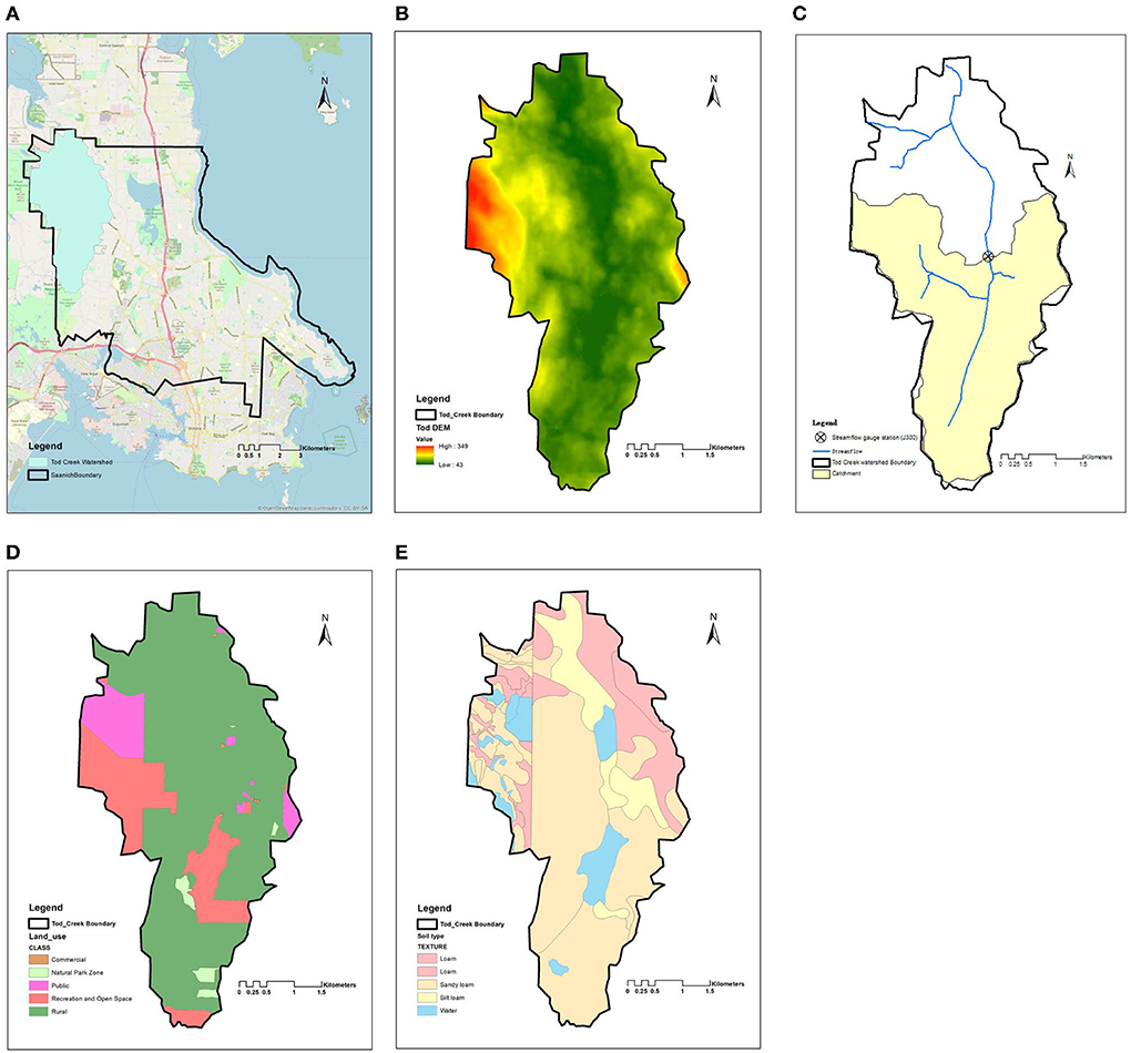
Figure 2. (A) Saanich area with Tod Creek draining to Saanich boundary in blue; (B) DEM image for the Tod Creek catchment; (C) watershed delineation for the portion of Tod Creek catchment modeled by PCSWMM (shown in yellow); (D) land use; and (E) soil type.

Meteorological data in the form of daily rainfall and daily evaporation (Supplementary Table 1) and daily mean, maximum and minimum temperatures were obtained from the Government of Canada open data website (https://climate.weather.gc.ca/historical_data/search_historic_data_e.html) for the Victoria Prospect Lake (101Q6NN) rainfall station. For the selected study area, rainfall data were only available for 1973-1986, and in this range, 1984 was deemed an average year and therefore, the period selected for model calibration. Temperature distribution curves were obtained from the nearby weather station (1018620) at the Victoria International Airport in Sydney, BC for the period of 1984. Data from 1960-90 Mean daily Evaporation (Walsh et al., 1995) are also used as input to PCSWMM, as shown in Supplementary Table 2. It should be noted that in the calibration period, the Tod Creek catchment had minimal urbanization estimated to be around 5% of the total area.

The Tod Creek watershed shown delineated in Figure 2B is 17.47 km²; however, the “Tod Creek below Prospect Lake” (08HA054) flow gauge station is used to delineate the catchment used in this research. The resulting catchment area draining to the gauge (henceforth referred to as J300 shown in Figure 2C) that is shown in Figure 2C in yellow is delineated using ArcGIS to be 10.38 km². This flow gauge has 9 years of flow discharge records (1982–1990) (08HA054). Note that the period of overlap with available rainfall data from the Victoria Prospect Lake rainfall station is only 1982–1986.

PCSWMM's LID model equations for bioretention cells

Bioretention cells are modeled by solving a set of simple flow continuity equations through three layers. As shown in Figure 3, only vertical water movement occurs within and between layers in bioretention cells. By considering the water balance of each individual layer, the rate of water transfer between the layers over time, expressed in mm/h, is determined. An inflow hydrograph to the LID unit is transformed into a combination of runoff, infiltration, subsurface storage, and subsurface drainage into the nearby native soil by numerically solving the continuity equation (Equation 1) at each runoff time step (Rossman and Huber, 2016).

FIGURE 3

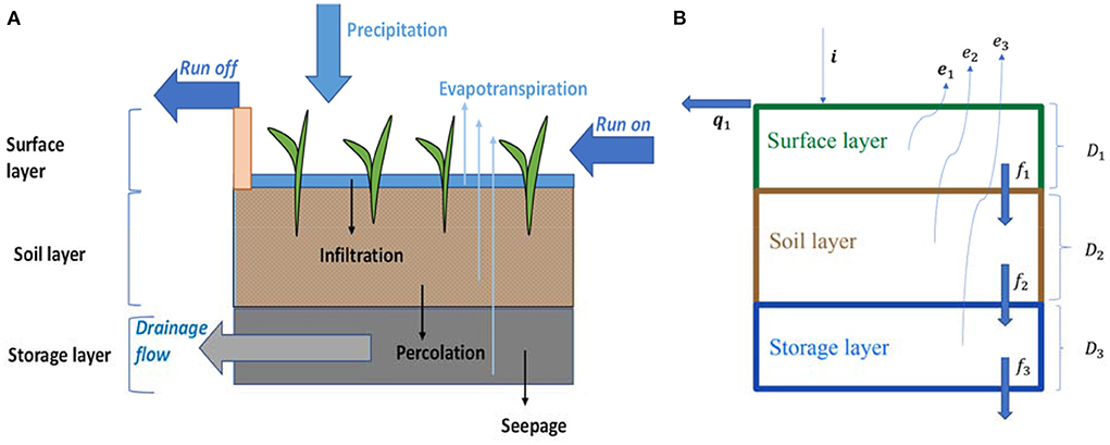
Figure 3. Typical bioretention cell: (A) representation in PCSWMM; (B) important variables and parameters (in Equations below and in the Appendix).

PCSWMM conceptualizes a subcatchment as a rectangular surface that has a uniform slope S and a width W that drains to a single outlet channel. Water balance is modeled using continuity such that:

$\begin{array}{llll}\frac{\partial d}{\partial t}& =& i-e-f-q& (1)\end{array}$

$\begin{array}{llll}q& =& {\alpha }_i{(d-d_S)}^{5/3}=\frac{1.0W{S}^{1/2}}{An}{(d-d_S)}^{5/3}& (2)\end{array}$

where i is the rate of rainfall plus snowmelt (mm/hr); e is the evaporation rate (mm/hr); f is the infiltration rate (mm/hr); q is the runoff rate (mm/hr) and d (mm) is the head of ponded on the surface (t is time in hr). The runoff rate is computed using Equation 2 where Wis the width for the rectangular area; d_S is the depth of the depression storage depth (and therefore, d−d_S is the net height of water leading to surface runoff); S is the uniform slope for catchment; n is Manning's coefficient; A is the surface area of the sub-catchment and α_i is defined in Equations 3a and 3b. The equations specific to the surface layer, soil layer and storage layer are given in the Appendix in Supplementary material.

PCSWMM divides the sub-catchment into three subareas (pervious subarea, impervious subarea, and zero-impervious subarea) and solves for the depth of each subarea separately. At the end of each time step, the runoff from each subarea is combined to determine the overall sub-catchment runoff. The difference between PCSWMM in calculating pervious area runoff and impervious area runoff is related to the difference in area and Manning's coefficient n based on land use. With regard to the pervious subarea, the coefficient α_i for the pervious subarea is:

$\begin{array}{ll}{\alpha }_1=\frac{1.0W{S}^{1/2}}{A_1{n}_P}& (\mathrm{3a})\end{array}$

where A₁ is the pervious subareas and n_P is the user designed pervious Manning's n. For impervious areas,

$\begin{array}{ll}{\alpha }_2=\frac{1.0W{S}^{1/2}}{(A_2+A_3)n_I}& (\mathrm{3b})\end{array}$

where A₂+A₃is the sum of impervious area and zero-impervious area and n_I is the user designed impervious Manning's n.

Surface runoff and flux constraints

It is assumed that any ponded surface water in excess of the maximum freeboard (or depression storage) height D₁ becomes immediate overflow,

$\begin{array}{ll}{q}_1=max\left[(d_1-D_1)/\Delta t,0\right]& (4)\end{array}$

where D₁ is the berm height for surface ponding (mm), and d₁ is the depth of water stored on the surface (mm). To ensure that at any given time step (Δt), the moisture levels in the soil and storage layers are not negative, nor exceeding the capacity of the individual bioretention cell layers, constraints are added to the bioretention cell layers to limit flux rates. Input values such as (D₂ and D₃) for these limits are to be provided by the user and the following equations are used in PCSWMM (variables are described in the Appendix, now in Supplementary material). Regarding the soil layer, the amount of the drainable water already present in the soil layer and the net amount of water added to it over the time step limits the soil percolation rate f₂. Here D₂ is the thickness of the soil layer (mm); θ₂ is the soil layer moisture content (volume of water/total volume of soil); θ_FC is the soil's field capacity moisture content.

$\begin{array}{ll}{f}_2=min\left[f_2,({\theta }_2-{\theta }_{FC})D_2/\Delta t+f_1-e_2\right]& (5)\end{array}$

Regarding the storage layer, the amount of unused volume in the storage layer and the net amount of water (D₃−d₃) taken from storage layer (D₃ is the depth of the storage layer and d₃ is the depth of water in the storage layer) over the time step both serve to limit the soil percolation rate. In the Equation (6), ϕ₃ is the void fraction of the storage layer (void volume/total volume).

$\begin{array}{ll}{f}_2=min\left[f_2,(D_3-d_3){\varphi }_3/\Delta t+f_3+q_3+e_3\right]& (6)\end{array}$

The volume evacuated by drainage and soil evaporation over the time step, together with the amount of accessible empty pore space, limits the soil water infiltration rate f₁.

$\begin{array}{ll}{f}_1=min\left[f_1,({\varphi }_2-{\theta }_2)D_2/\Delta t+f_2+e_2\right]& (7)\end{array}$

Clogging factor

Clogging can decrease a bioretention cell's hydraulic conductivity K with time. A clogging factor (CF) is defined in the model as the amount of layer void volume that experiences complete clogging in the layer, and it is assumed that the conductivity is lost linearly with the amount of clogged void volume. Then K at a particular time t can be determined as follows:

$\begin{array}{ll}{K}_{3S}(t)=K_{3S}(0)\left(1-\frac{Q(t)D_3{\varphi }_3}{CF}\right)& (8)\end{array}$

where K_3S(0) is the initial saturated hydraulic conductivity of the soil; CF is the clogging factor for the entire bioretention cell; Q(t) is the cumulative inflow volume per unit area of the LID at time t:

$\begin{array}{ll}\begin{array}{l}Q(t)={\displaystyle {\int }_0^t(i(\tau )+q_0(\tau ))d\tau }\hfill \end{array}& (9)\end{array}$

where i(τ)+q₀(τ) is the rainfall plus captured runoff inflow to the LID accumulated up to time t and τ represents time in the integrand.

Clogging only applies to simulations lasting several months or longer because it is a long-term process. PCSWMM assumes that clogging, or the decline in infiltration rates for bioretention cells, happens at a constant rate proportional to the quantity of void volumes that the LID unit treats over time. The number of years (T_clog) it takes to fractionally drop infiltration rate to a degree F_clog can be used to calculate the clogging factor. The CF is computed using the following formula:

$\begin{array}{ll}CF=\frac{I_a(1+R_{LID})T_{clog}}{{\varphi }_3{D}_3{F}_{clog}}& (10)\end{array}$

where I_a is the annual volume of rainfall in inches; R_LID is the unit's capture ratio; T_clog is the number of years; and F_clog is the degree of decrease for an infiltration rate.

PCSWMM applied to the Tod Creek catchment

Tod Creek below Prospect Lake streamflow station (08HA054) was used as an outfall to delineate the lumped catchment (referred to as catchment A) shown in Figure 4A. Figure 4B shows the three sub-catchments (indicated as B1, B2, and B3) also delineated by ArcGIS for the purposes of spatial scaling exploration. Catchment A is 10.38 km², B1 is 4.86 km², B2 is 2.51 km² and B3 is 3.01 km². The land use information shown in Figure 2D is used to determine parameters, such as impervious and pervious percentages, D_store imperviousness and perviousness, and zero-imperviousness percentage. We selected the Green-Ampt method for infiltration, and the soil information shown in Figure 2E provided the suction head, conductivity and initial deficit by weight of area.

FIGURE 4

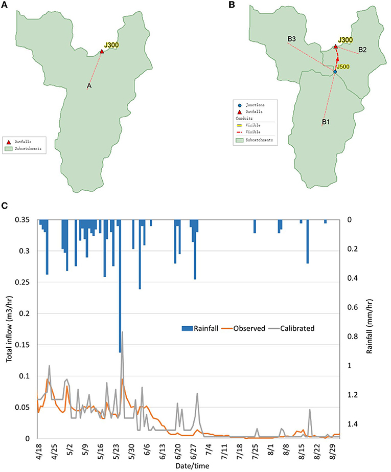
Figure 4. (A) Tod Creek draining to J300 showing catchment A; (B) Proposed sub-catchments B1, B2 and B3; and (C) Hyetograph and calibrated and observed flow curves for modeling flow at J300.

In order to identify the values of soil related parameters and other fixed features that do not change in time or space (such as overall catchment area and soil type for example), PCSWMM was calibrated using the Nash–Sutcliffe efficiency coefficient (NSE) and the coefficient of determination (R²). The daily rainfall data from the Victoria Prospect Lake (101Q6NN) rainfall station close to J300 for the April to October 1984 period was used with the 08HA054 flow data to calibrate the model applied to the lumped catchment A. The land use data obtained was released in 2004, and after considering land use changes over the past 20 years in the region, we assigned a uniform percent imperviousness of 5% for the calibration period in 1984. The size of the baseflow flowing into J300 is set according to observed data at the flow gauge. It is worth noting that in January, February, March, November, and December, the baseflow is not 0, and the values of the baseflow before and after calibration are shown in Supplementary Table 3. In addition, the temperature data in 1984 fell below 0°C prior to April and hence, the calibration period was taken as April 15^th to September 29^th, which is outside the snow period. Calibration focused on matching peaks in the hydrograph (shown in Figure 4C) as closely as possible as well as overall volumes. The calibration was conducted at a daily time step given the rainfall hyetograph shown in Figure 4C.

PCSWMM's internal Sensitivity-based Radio Tuning Calibration (SRTC) tool allows the user to select initial values for control parameters, as well as specify uncertainty levels. This tool was used to calibrate various parameters, particularly those related to soil type. Parameters affected by soil type are suction head (calibrated to 3.976 mm), hydraulic conductivity (calibrated to 0.872 mm/hr) and initial deficit fraction (calibrated to 0.298). In addition, we also calibrated the monthly distribution of the baseflow, and the calibrated and observed hydrographs are shown in Figure 4C. The final NSE value was 0.69 [considered “good” according to Moriasi et al. (2007)]. We use these calibrated soil parameters and the baseflow pattern for subsequent modeling analysis. It is worth noting here that since the time interval of our rainfall data is 24 h, extreme values will be poorly modeled in comparison to minute or hourly data (which were not available for the study region). The main point of the calibration was to capture the monthly distribution of J300 baseflow as well as soil related and land use parameters. The final calibration parameters are given in Supplementary Table 4.

Minimal urbanization scenarios for 50-year return period rainfall and timeseries rainfall

Intensity-Duration-Frequency (IDF) curve data for the 50 year design storm is obtained from Environment Canada (https://climatedata.ca/resource/idf-curves-and-climate-change/) for the Victoria International Airport Meteorological station (1018620). The rainfall distribution for the 50 year design storm is the Chicago distribution type and is shown in Figure 5A. The authors applied the calibrated model with the 50-year return period rainfall storm and the response is also shown in Figure 5A. The bioretention cell saturation level is set to 75% before the storm, and the catchment area's impervious ratio remains at 5%.

FIGURE 5

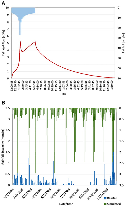
Figure 5. (A) Hydrograph of calibrated model using 1984 land use case (5% urbanization) for the 50-year return period rainfall event (rainfall shown on the upper horizontal axis); and (B) continuous hydrological times series used in temporal scaling and model verification analysis.

Figure 5B shows a continuous time series rainfall data from 1986 that is used in the temporal scaling investigation as well as in the model verification portion of this research. When comparing the 1986 rainfall data to the 1981–2010 Climate Normal, the 1986 rainfall is a relatively wet year being 21% wetter than usual overall. The temperature was average according to the 1981–2010 Climatic Normal. Also shown in Figure 5B is a simulated rainfall data set created using the real rainfall data of 1986. This was done to test the effects of dynamic parameters that change bi-monthly. The reason for creating the simulated rainfall series is because the real rainfall data series of 1986 had periods of little-to-no rain, making it impossible to see the flow response in these periods given changing parameters. Thus, for those months where rainfall was absent, the rainfall from wet sub-periods within 1986 were simply replicated for the dry sub-periods as shown.

Scenarios investigating spatial scaling impacts

This part explores the impact of the percentage of LID (to the total area) in the catchment as well as the impact of spatial heterogeneity and discretization. Considering future urban planning for the area, we speculate a future impervious area to be 40% in the not to distant future, as shown in Table 1.

TABLE 1

Table 1. The scenarios setting for spatial scaling impacts analysis.

Sensitivity to temporal scaling: Static and dynamic parameter changes

The model was applied using the real continuous rainfall series of 1986 (shown in Figure 5B) but only for lumped catchment A, for an LID area of 5% of the catchment and using calibrated values that remain static for the entire time period. For continuous simulations, the initial saturation level is set to 25%. To model the impacts of what should be dynamically changing parameters affecting each layer, the Authors chose to model bi-monthly periods in 1986 where certain parameters are altered for each of those periods. In addition, because 1986 has various dry periods in the mid to late summer that are not useful for analyses, the authors created a simulated rainfall event by repeating the rainfall in the first period for three more periods, and repeating the November rainfall up to July-Aug. This is the simulated rainfall shown in Figure 5B. Table 2 below illustrates the dynamic parameter changes for each layer.

TABLE 2

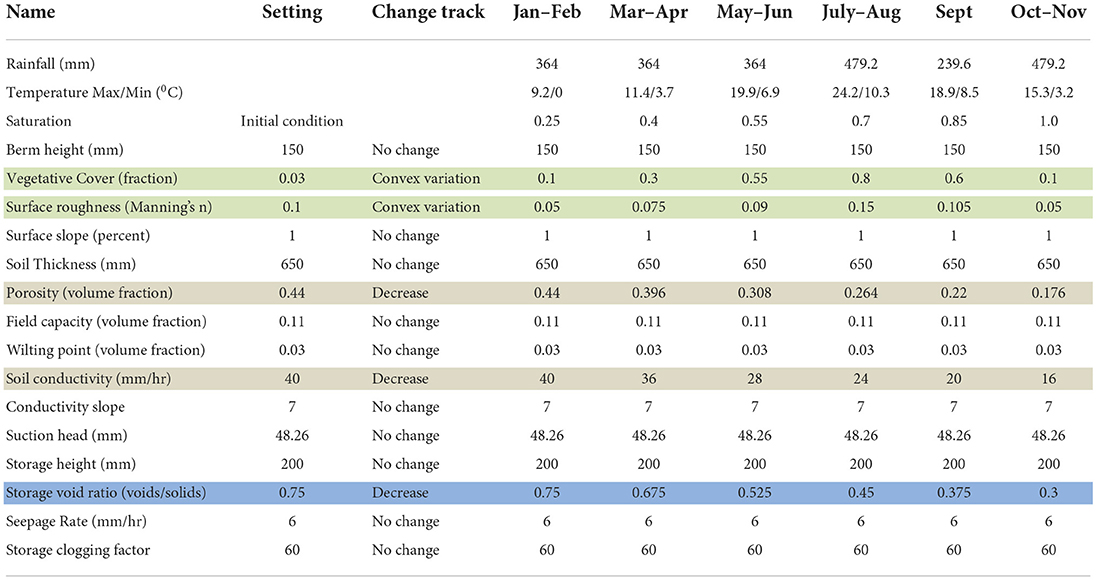
Table 2. LID parameter changes in dynamic LID parameter analysis with surface layer parameters shown shaded in green, soil layer in light brown, and storage layer dynamic parameter changes in light gray.

For all scenarios noted in Section Scenarios investigating spatial scaling impacts and Section Sensitivity to model concepts: Defining a range of LID parameters, LID performance is assessed using the conventional formula shown in Equation 11a. The Authors propose an additional equation for calculating LID performance and shown in Equation 11b.

$\begin{array}{ll}P=\frac{S{O}_{NoLID}-S{O}_{LID}}{S{O}_{NoLID}}\times 100\%& (\mathrm{11a})\end{array}$

where P is the performance metric describing the percent reduction (or increase) associated with the computed output (either peak flowrate or total volume); SO_{No LID} is the computed output after urbanization with no LID implemented; S_LID is the computed output after urbanization in the various scenarios. The following alternative equation for performance is proposed and also used in this work:

$\begin{array}{ll}{P}_{LID}=\frac{S{O}_{NoLID}-S{O}_{LID}}{S{O}_{NoLID}-S{O}_{Pre-Urban}}\times 100\%& (\mathrm{11b})\end{array}$

where SO_Pre−Urban is the computed output before any urbanization. This performance metric helps to shed light on the ability of the LID to return the catchment to pre-urbanization levels.

Sensitivity to model concepts: Defining a range of LID parameters

The SA in this work uses parameter ranges and user assigned uncertainty to determine model sensitivity to parameter changes. The uncertainty ranges shown in Table 3 for each parameter, were devised based on the following expressions given by PCSWMM using the SRTC tools:

$\begin{array}{llll}{R}_{Low}& =& R_{Current}\times \left(\frac{1}{1+U/100}\right)& (\mathrm{12a})\end{array}$

$\begin{array}{llll}{R}_{High}& =& R_{Current}\times \left(1+\frac{U}{100}\right)& (\mathrm{12b})\end{array}$

where R_Low is the lower bound for parameter's uncertainty range; R_High is the upper bound for the parameter's uncertainty range; R_Currentis the current parameter's setting; and U is the uncertainty percentage assigned by the user (we selected 100%). Table 3 describes the parameter settings corresponding to the default bioretention cell values and the uncertainty ranges determined with Equation 12. The variations in modeling results (i.e., peak flowrate and total volume for the 50 year rainfall event and total volume for the real continuous rainfall series of 1986) are assessed for a specific percentage change in each input change. This process tests the sensitivity of the model to uncertain inputs. For the 50 year rainfall event modeling, we set to initial saturation level to 75% and for the real, continuous rainfall data series of 1986, the initial saturation level is set to 25%. Because bioretention cells are mainly divided into three layers, the basic settings of each layer are derived from Low Impact Development Stormwater Management (2022). The SA settings are given in Table 3.

TABLE 3

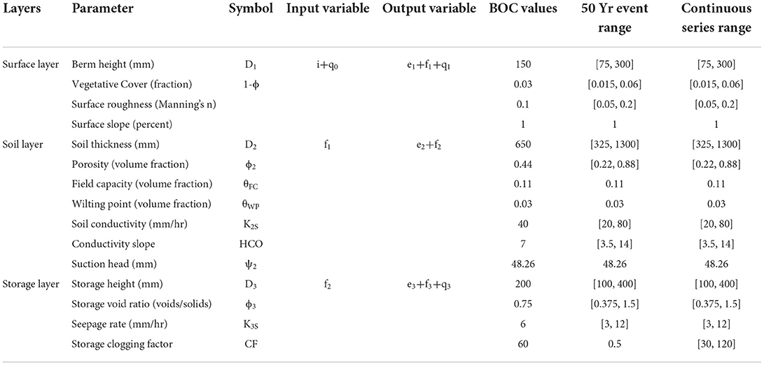
Table 3. LID initial assignment parameter table, and sensitivity analysis range for event and continuous rainfall.

Metrics for LID performance and SA affected by spatial scale

PCSWMM computes what is referred to as the “average normalized sensitivity” and given in Equation 13. This sensitivity is computed by dividing the difference between the largest and smallest objective output (the objective function is either peak flowrate or total volume) by the objective function value associated with the BOC's parameter value.

$\begin{array}{ll}{N}_i=\pm \frac{|Max{O}_i-Min{O}_i|}{O_{BOC}}& (13)\end{array}$

where i is the LID parameter; MaxO_i is the largest objective function value computed for the uncertainty range assigned to that parameter (Table 3); MinO_i is the smallest objective function value over the uncertainty range; O_BOC is the BOC's objective function value for that range; and N_i is the average normalized sensitivity value provided by PCSWMM. In this work, we run simulations using the information in Table 3 to assign the uncertainty range for each parameter and record the PCSWMM output for the suite of N_i values for all parameters. These are then ranked to understand relative dominance of parameters in the simulations.

To explore model sensitivity to scaling and parameter uncertainty, a spatial dynamic sensitivity analysis (SDSA) is proposed in which the following metric is plotted versus LID implementation area (which is a measure of scaling in this work):

$\begin{array}{ll}\begin{array}{l}SDS{A}_i^j=\pm \frac{N_i^j{(R_{BOC})}_i^j}{{(R_{High}-R_{LOW})}_i^j}\hfill \end{array}& (14)\end{array}$

where i is the LID parameter; j is the LID implementation area scenario; $N_i^j$ is the average normalized value for parameter i (given by Equation 13) for the LID implementation area scenario j; ${(R_{BOC})}_i^j$is i^th parameter value for the BOC case shown in Table 3 and scenario j; and ${(R_{High})}_i^j$ and ${(R_{Low})}_i^j$ are defined in Equation 12 for parameter i, scenario j, and $SDS{A}_i^j$ is the metric that is plotted versus LID implementation area. Sensitivity is normally defined as a change in output for a given change in input $(\frac{\Delta y}{\Delta x})$. Equation 13, which provides N_i for each parameter is effectively $\frac{\Delta y}{y_0}$, which is likened to the performance metrics shown in Equation 11. The metric given in Equation 14 is proposed because it combines the conventional definition of sensitivity with PCSWMM's average normalized sensitivity. Plotting $SDS{A}_i^j$ vs. LID implementation area for each scenario j, provides a visual tool by which to assess the dynamics in parameters with spatial scale.

Results and discussion

Impact of spatial scaling

As shown in Table 1, AS0 is the scenario that uses the lumped catchment with 40% imperviousness and no LID implemented – this represents the BOC in this part of the analysis. The results of scenarios AS1 to AS7 as reductions in volume and peak flowrate computed using Equation 11a are shown in Figure 6. Also shown are the various water balance variables for each layer for the first four scenarios. The figure only shows LID area percentages up to 15% as there was no impact beyond 10% because implementing 10% of the total area as an LID brought the system back to pre-developed response. Hence only values up to 15% are shown. The reason that only 10% of LID area is required to bring the response back to pre-developed levels is for the simple reason that the bioretention cell is modeled as a single reservoir within the catchment. The LID area of 10% effectively captures all the water that is provided by the 50 year rainfall event. A 10% area amounts to 1 km² for catchment A, which for all intents and purposes, is a very large bioretention cell that is not often seen in practice.

FIGURE 6

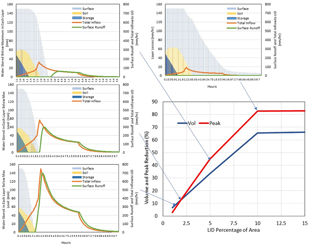
Figure 6. The basis comparison results for different scenarios in AS0–AS7. The horizontal axis in the figure at bottom right represents the implementation percentage of LID in the overall area, and the vertical axis represents the percent reduction. The smaller panels show the hydrograph components for scenarios AS1, AS2, AS3, and AS4.

The graphs also show the contributing amount provided by each layer. The total inflow to the bioretention cell is the red line and the response, or surface runoff from the cell is shown as the green line in the panels depicting the contribution to volume and peak reductions. As the amount of LID area increases, the volume reduction is a linear phenomenon whereas the change in peak rise more quickly with the change in LID percentage. As well, the contribution by the storage layers is relatively constant for increasing LID, the contribution by the soil layer increases somewhat, but it is the surface layer that contributes to the bulk of the response. This is consistent with the model's representation of the bioretention cell in which the surface provides the initial and immediate water “treatment” and it takes time for the water to reach the lower depths. The storage layer impact is seen later in the hydrographs. The soil layer functions as a buffer between the two other layers, contains the vegetation roots, and provides additional water quality treatment.

Figure 7 illustrates the impact to peak flow and volume (computed using Equation 11a) for the individual sub-catchments (scenarios B1,2,3 for each of S1 to S7 compared to S0). It is important to note that while the soil type had some variation, the greatest difference in the three sub-catchments is their physical characteristics, i.e., area, elevation change and shape. Hence, Figure 7 performance metrics is computed as a percent reduction in flow contributing to J300 per area of the sub-catchment (that is, Equation 11a divided by the sub-catchment's area). Hence, this analysis illustrates the impact of the “width” of the catchment, its slope and any routing experienced by the flow (and thus, the outlet of the sub-catchment's distance from J300). The differences between each sub-catchment are given in the Table 4.

FIGURE 7

Figure 7. Reductions normalized by subcatchment areas for peak flow and total volume.

TABLE 4

Table 4. Physical properties of each sub-catchment.

PCSWMM models a catchment as a rectangle with a width W, which is effectively the length of the water flow path length from the most upstream point to the outlet. Where the bioretention cell is located in the sub-catchment is in fact irrelevant, and thus the only topology and spatial heterogeneity considered in the model are the characteristics shown in Table 4. B1 is the headwater catchment and it is also the largest. B2 is the smallest sub-catchment with B3 being just slightly larger than B2. The smallest sub-catchment B2 contributes the most to peak flow reduction (comparatively), with the largest sub-catchment B1, the headwater catchment, providing the least reduction per area. This trend is also true when LID area is 5% or more. This trend is reversed however, for lower LID areas less than 5%. These changes in relative reductions for varying LID area arises because of the elevation across the rectangle that represents the sub-catchment in PCSWMM. B3 has the highest slope for the shorter flow path length than the other catchments. This suggests that implementing LIDs in areas of rapid flowrate generation may contribute to a greater calculated reductions in overall volume than in flatter, larger sub-catchments such as that in B1. The changes in soil type are likely only marginal contributions to the differences observed.

Obviously, LID area is one of the largest influencing factors in the LID response. Figure 8 is an illustration of how even small increments in area impact flow peaks and volumes. It illustrates the impact of increasing the LID implementation area in smaller increments (starting from 2.5%) than shown in the previous graph. The J300 observation volume reductions increase linearly with the area, which makes sense as storage volume grows linearly with area because the depth is fixed. The impact to peak flow, however, increases in a somewhat undulating fashion suggesting a relative tradeoff between the different parameters as the bioretention cell area increases. The results show that an LID's ability to reduce peak flow varies at different LID implementation scales. When the LID area is small, the surface layer, soil layer, and storage layer of the LID are filled quickly with stormwater generated from the upstream impervious surfaces. At the surface, Manning's n can influence the response since the LID is much rougher than the impervious areas. By increasing the net LID area, one reduces the imperviousness and changes the overall roughness, thereby reducing peak flow. This apparent reduction in peak flow; however, decreases as the area increases leading to a somewhat convex shape. As the area of LID increases, the soil layer and storage layer begin to play a more prominent role, and the surface runoff generated gradually changes with increasing scale, hence causing an undulating pattern in the peak flow curves of Figure 8. When LID area is over 10%, there is negligible surface runoff generated because of the bioretention cell, and the runoff through J300 comes only from the pervious area. Similarly, research using the SWMM5 model to retrofit existing gray infrastructure in Italy showed that there was a threshold value of area (in percent of total catchment area) retrofitted with LIDs. Increasing the LID area above this threshold led to only marginal gains in hydrological benefits (D'Ambrosio et al., 2022).

FIGURE 8

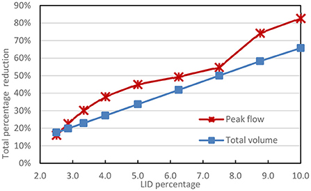
Figure 8. Sensitivity analysis for LID area changing with respect to J300 flowrates and volumes. BOC is 5% with percentage increments from 2.5 to 10% LID area. Simulations are conducted using the 50 year event on lumped catchment A.

Impact of temporal scaling

Figure 9 shows runoff coefficients for catchment A, scenario 3 (5% of the area is covered with a bioretention cells) using the simulated 1986 rainfall for the parameters in Table 2. The changes by layer are also shown with the same colors depicted in Table 2 indicating the different layers. The surface layer is dominated by vegetation in the summer period and a high roughness. Relative to the BOC case (the black lines) using static parameters in this simulation, the influence of vegetation is to effectively increase runoff (as the runoff coefficient is just slightly higher in the summer months). This seems counter-intuitive and this is because of the manner in which PCSWMM uses vegetation in the model's concepts (Lisenbee et al., 2021). In PCSWMM, vegetation is simply a mechanism that reduces potential storage volume in the surface. However, the effect is minimal demonstrating that the vegetation in bioretention cells is not a significant factor in bioretention cell function according to the model.

FIGURE 9

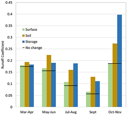
Figure 9. Runoff coefficient for each period in which there is a change in surface, soil or storage parameters. The black line indicates the static parameter runoff coefficient for the sub-period.

The soil layer changes are resulting from a progressive but quite drastic decrease in hydraulic conductivity, and porosity over the year. The soil layer's contribution to raising the runoff coefficient increases throughout the year as progressively higher amounts of water go to saturating the soil quickly and generating runoff under the very wet simulation that receives rainfall in every bi-monthly sub-period. The runoff coefficient is highest when everything is completely saturated in the final sub-period of Oct-Nov.

The storage layer is impacted in the dynamic simulation by a reduction in voids available to store water. In the continuous simulation after a long, wet period, storage is the biggest influence on water volumes when the soil is saturated and the void ratio has diminished due to continual clogging. To further explore the impacts of each layer's dynamics on water volume, Figure 10 illustrates the deviation from the static case in either water balance terms (left column) or impact on total volume that is contributed by each of the layers (right column). Noting that this is a simulation with 5% coverage of bioretention cell area, there should be significant reductions in flow overall as observed in the earlier graphs.

FIGURE 10

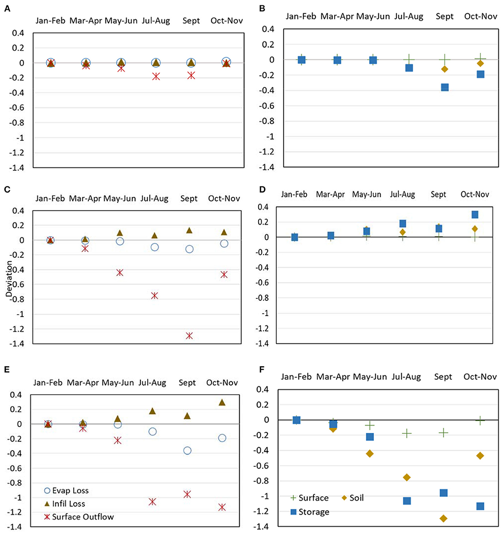
Figure 10. Results of dynamic changes of selected parameters over time. Left column illustrates influence on water balance and outflow from (A) surface layer; (C) soil layer; and (E) storage layer for the time period. Right column illustrates influence of different parameters relevant to the different layers on: (B) evaporation loss; (D) infiltration loss; and (F) surface runoff.

Different than the event simulations, the surface layer contributes very little to surface runoff or evaporation (Figures 10A,B,F). The Hargreaves method of estimating evaporation in PCSWMM was used to calculate the contribution to evaporation (considered to encompass both evaporation and transpiration processes by the model) for the water balance. However, the vegetation seems to have little impact on the water balance components over time. Only the storage layer is affected by evaporation (Figure 10B). This layer is the deepest layer and as Figure 3B shows, it contributes to the bulk of evaporation by simple virtue of the fact that that is where the water supply for evaporation is stored. Regardless of the impact of the soil layer and the surface layer to hinder or promote evaporation, the model considers this a loss from storage in the transmission of water from the cell (which is restricted to the vertical direction). Figures 10C,D show the influence of soil layer and infiltration mechanisms in overall water balance. The soil layer seems to directly contribute to surface runoff but overall, infiltration is not an influencing mechanism in the dynamics. Figures 10E,F show that the storage layer is the dominant layer in continuous simulations. Total volumes are of interest in continuous simulations and the storage layer contributes greatly to the resulting surface runoff, suggesting that for continuous modeling, bioretention cells designed with this model, could simply be comprised of a single layer – the storage layer.

Verifying model concepts

In this section, Equation 11b is used to test the model's sensitivity to given parameter uncertainties (shown in Table 3) in terms of performance metrics. The performance metric corresponding to each parameter in the event simulations is computed using peak flow and volume output; but only volume output is computed with Equation 11b when running continuous simulations. All parameters are static in the continuous simulations.

Sensitivity analysis using a single rainfall event

In this analysis, catchment A with a 5% bioretention cell coverage under a 50 year rain event is simulated to determine the sensitivity of the bioretention cell's performance to each of the parameter uncertainty ranges shown in Table 3. Figure 11 involves radar charts showing how parameter influences vary relative to each other overall (Figures 11A,B, for peak and volume, respectively), surface layer parameters only are shown in Figures 11C,D, soil layer parameters in Figures 11E,F, and storage layer parameters in Figures 11G,H, for peak and volumes, respectively.

FIGURE 11

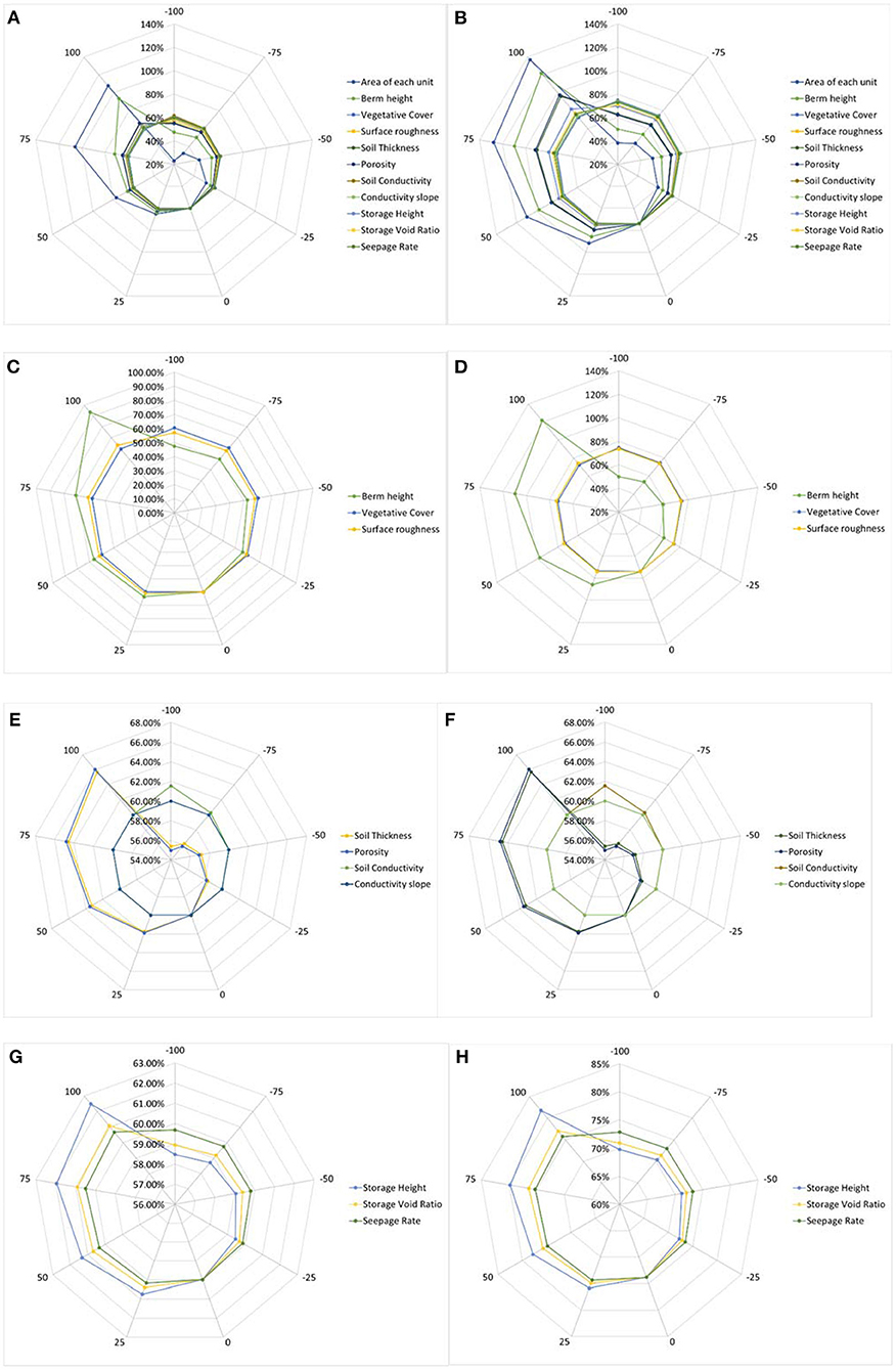
Figure 11. Influence of bioretention cell parameters in the 50 year rainfall event, 5% LID coverage in catchment A on mitigating: (A) peak flow and (B) volume; influence of surface layer parameter on mitigating (C) peak flow and (D) volume; influence of soil layer contributions for mitigating (E) peak flow and (F) volume; and influence of storage layer on mitigating (G) peak and (H) volume.

The radar charts show the relative influence between parameters in these simulations. Figures 11A,B, not surprisingly, show that the area and the berm height in the surface layer affect the peak runoff in event modeling as well as the volume. Other parameters have a larger impact on volume mitigating performance than they do on mitigating peak flow. This is consistent with bioretention cell design and within the model. Figures 11C,D show the influence of vegetative cover and surface roughness in the surface layer parameters. They display only a 50% impact for a 100% change in the parameter values, rendering these parameters somewhat insensitive. The model is highly affected by changes in berm height particularly for larger increases. Figures 11E,F show that all soil layer parameters are not very impactful to peak or volume, although, the model is slightly more sensitive to soil thickness and porosity than the other two parameters. Figures 11G,H show that peak flows resulting from flood events are relatively insensitive to storage layer parameters while the volume is somewhat affected by the storage height. Thus, for flood events, the surface layer parameters are the most impactful. In a flood event, the surface layer will accumulate and the berm height determines the water storage capacity of the surface layer. Surface runoff is automatically generated when this height is exceeded. Besides, raising the vegetative cover increases the total volume and peak flow, and lowering the vegetative cover will lower the total volume and peak flow. The increase in vegetative cover will reduce the internal water storage available in the soil layer, so that only a small portion of the water is retained in the voids of the soil layer, thus, increasing overland flow. The change of surface roughness has almost no effect on the total volume, but the increase of the Manning coefficient will reduce the overflow rate, so the effect of increasing this parameter is to reduce the peak flow.

Regarding the soil layer parameters, the performance of the bioretention cells is somewhat sensitive to soil thickness, and porosity but not sensitive to field capacity and conductivity slope. The soil's field capacity determines the minimum soil moisture content below which percolation will not occur. However, during this rainfall event, the soil moisture content of the upper surface layer was always greater than that of the soil layer, so percolation always occurred. Changing this value will have no effect on the flow observed at J300.

Similarly, increasing the porosity of the soil layer can reduce, as well as delay the peak flow timing and reduce the total volume. Conversely, reducing the porosity will increase the peak flow, quicken the runoff peak's time, and increase the total volume. If the porosity is reduced to 0, this will mean that the current bioretention cells are only functioning as a ponded layer. Thus, the bioretention cells will become a small pond that slows the peak time but does not fully perform the intended function of a bioretention cell. Decreasing the percentage of soil conductivity will advance peak flow timing and increase peak flow size. For the current LID setting, the soil conductivity is set to 40 mm/hr, and if this value continues to decrease, it will cause rainfall to enter the storage layer from the ponding layer at a slower rate. The accumulated water in the surface layer will become overland flow. The suction head is derived from the soil conductivity, so we did not analyze the influence of the suction head.

Storage heights can also influence response to rainfall events. Increasing the vertical height and storage void ratio of the storage layer will allow more water to be stored in the bioretention cells, thus reducing total volume and peak flow. Besides, it is observed that increasing the seepage rate will increase the infiltration loss of the original soil, thereby reducing the total volume and peak flow. The clogging factor is only intended to function in continuous rainfall events over extended periods of time.

To illustrate the relative dominance of the parameters in terms of model sensitivity, the Authors used Equation 13 (N_i) to create Figure 12. Dominance is measured relative to a specific objective function, i.e., the total volume of peak flow, from pervious and impervious areas as well as the total volume computed at J300. The results show that in the AS3 scenario, the LID area implemented is the dominant factor affecting the total volume and peak flow. After area, Figure 12 shows that there is really only one factor (out of 11 tested) that dominates the LIDs ability to reduce peak flow (relative to the other parameters): berm height, which is a surface layer parameter. Total volume reductions are dominated by berm height, porosity, and soil thickness, with the last two being soil layer parameters. This is consistent with how bioretention cells are intended to function for short-term floods. Figure 13 shows the SDSA plot of Equation 14 for the parameters shown in Figure 12 (and for the same event simulation) as a function of the area of LID implemented. This helps to illustrate scaling related effects on model sensitivity. Figure 13 shows that the SDSA metric values for peak flow (Figures 13A,B) and volume output (Figure 13C).

FIGURE 12

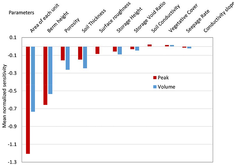
Figure 12. Ranking parameters based on Equation 13 for bioretention cell response to the 50-yr rainfall event on AS3 (entire catchment with 5% LID coverage).

FIGURE 13

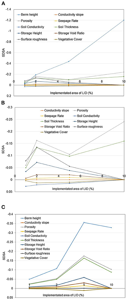
Figure 13. SDSA values vs. LID implementation scale for scenarios AS1 to AS4 for (A) for peak flow; (B) for peak flow but excluding berm height; and (C) for total volume.

In Figure 13, the results show that flood event reduction is most sensitive to berm height for both peak flow and total volume within the sensitivity range used (Table 3) at all scales. It is worth noting that N_i of Equation 13 used in Figure 12, is only meaningful within each LID area implementation scenario making it challenging to infer trends across LID implementation scales. But this is possible when using SDSA plotted in Figure 13 because this sensitivity metric combines the model's performance with the change in output given the change in parameter input for a specific LID area. This facilitates visualizing the relative role of the various parameters to performance over LID size.

Figures 13A,B show that the parameters' influence on performance fluctuates with the LID area, especially between 1 and 2%. This observation shows that when LID is implemented in small areas, changing the Manning coefficient (surface roughness) is relatively more effective than changing the berm height (in the uncertainty range assigned). As the LID implementation area increases, the overall LID water storage capacity tends to increase and the parameters affecting the LID's ability to reduce peak flow are mostly influenced by berm height. Increasing this value can reduce the formation of surface runoff, which is more efficient in reducing the peak flow than other LID parameters. Figure 13B eliminates the berm height curve to better illustrate the relative roles for all the other parameters across scales. The figure shows that the soil layer's porosity and hydraulic conductivity as well as surface roughness shift relative to each other when LID area is between 1 to 5%. At the smallest scales, the surface roughness actually has a greater influence on performance than the other parameters; but with just a little more area and scaling up, porosity, a soil layer parameter, dominates the performance. In terms of mitigating peak flows in flood events, the results show that the parameter designs should focus on berm height when scaling up to larger LID areas.

For influences on total volume reduction objectives (Figure 13C), the results show that no matter how the area changes, berm height is always the most influential parameter for flood events. Unlike Figure 13B, there is no change in relative positioning of parameter influences across LID area (i.e., the lines do not cross each other as they do in Figure 13B). However, the slopes of the trends in Figure 13 change depending on the change in LID area. Figure 13C shows that when the initial LID area is small, and regardless of the uncertainty in LID parameters, the LID will store all water in its surface layer in a relatively short period of time, and given the initial LID saturation of 75%, the storage layer is relatively insignificant across scales. The soil layer's porosity and thickness are the two most important parameters outside of berm height in this figure, but the role that porosity and thickness play in the physical representation of the bioretention cell results in modeling the soil layer as simply a reservoir with a net depth. There is no real influence from soil hydraulics nor is there a meaningful role for soil in that layer – it is just another reservoir. As the area increases, each layer's storage capacity (i.e., reservoir size) increases correspondingly; the surface runoff formed by the LID gradually decreases, the peak flow decreases and so does the total volume of runoff. Figure 13 shows that physically-based parameters play a significant role in performance for smaller (less than 5%) LID implementation areas, suggesting that PCSWMMs model concepts for bioretention cells lose their physicality as LID area increases. This is because the increase in LID area amplifies the water storage capacity of the LID such that it can be modeled as a simple tank, and other more physically-based parameters related to soil type or vegetation have marginal influences on the physics behind the LID's performance. The horizontal axes in Figure 13 all stop at 10% because LID areas in excess of 10% are unnecessary as runoff is no longer generated in the catchment.

Sensitivity analysis using a continuous time series

The above findings have shown that LIDs perform well when dealing with a single, large rainfall event that could potentially lead to flooding. However, bioretention cells should be designed to be functional over long-term, continuous rainfall events. The 11-month rainfall data observed in 1986 (shown in Figure 5B as the blue hyetograph) was used to conduct a similar analysis to Section Sensitivity analysis using a single rainfall event but for a long-term simulation that only considers impact on total volume. Equation 11b is used with scenario AS3 to create Figure 14. Figure 14A shows all the parameters, while Figures 14B–D show the sensitivity of volume predictions to surface parameters, soil parameters, and storage parameters, respectively. As seen previously, for continuous simulations, the storage layer is the most important layer in affecting response. But more importantly, the clogging factor that was discussed in Section Clogging factor is enormously influential in continuous simulations. The volume capacity of the storage layer is directly affected by the clogging factor, which describes the rate at which the bioretention cell clogs over time. Figure 15 ranks the values of average normalized sensitivity (from Equation 13) for this simulation. It confirms that clogging factor is second after storage depth in terms of importance in mitigating total volume in continuous simulations. It is worth noting that clogging factor was set to 0.5 during the short-term rainfall events simulations (Table 3), indicating that the bioretention cells would clog within a short period of time. The clogging factor for the continuous simulation (as shown in Tables 2, 3) was set to 60, which indicates that the bioretention cell will ultimately lose its ability to infiltrate water to the native soil in about 2 years. Examining the observed rainfall at the end of 1985 (the year previous to the 1986 rainfall data), December was dry, and the latter half of November was also dry. As a result, we set the initial saturation to 25%. In terms of total volume, increasing LID implementation area will also effectively mitigate the impact of urbanization as it did for large, short-term rainfall events. However, in terms of temporal scaling, the impact to total volume mitigation in short-term rainfall events was dominated by parameters in the surface layer and some soil layer parameters. Storage layer parameters were not a factor. Conversely, for long-term rainfall events, the storage layer is much more significant than that of the soil and surface layers in PCSWMM. Clogging factor, which is a storage layer parameter, along with parameters related to native soil, play a more significant role in representing the physics behind performance over longer time series. Therefore, evaluating the performance of LIDs should not be limited to short-term, flood events but should be assessed under long-term rainfall events.

FIGURE 14

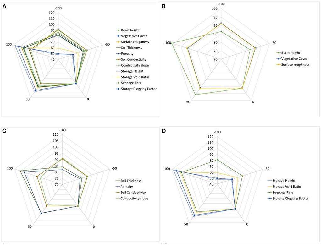
Figure 14. The influence on bioretention performance (computed using Equation 11b) in AS3 and continuous timeseries rainfall from (A) all parameters; (B) surface layer parameters; (C) soil layer parameters; and (D) storage layer parameters.

FIGURE 15

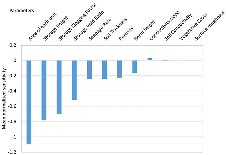
Figure 15. Ranked average normalized sensitivity (computed using Equation 13) for 1986 continuous times series rainfall in AS3.

Table 5 shows the effect of clogging on predicted flow at J300 in the AS3 scenario. When analyzing time series, if the influence of the clogging factor is not considered (effectively set to 0), a final total volume obtained is 1,302,000 m3. If the clogging factor is set to 60, the total water volume computed at J300 is nearly double that: 2,076,000 m3. The shows that when we consider long-term rainfall events, setting a “reasonable” value of clogging factor is essential; however, there is no guidance on what this value is, other than it depends on a maintenance cycle, which can be difficult to do where bioretention cells are concerned. The attention to clogging has often been ignored by previous studies (Ahiablame and Shakya, 2016; Gülbaz and Kazezyilmaz-Alhan, 2017a; Bond et al., 2021) and is likely why the performance ability of LIDs has been overestimated in previous research (Lee et al., 2015; Conley et al., 2020). Similarly, when performing event-based rainfall analysis, one should also consider clogging because a small clogging factor can simulate surface sediments being washed into the bioretention cell system during high intensity rainfall, resulting in rapid infiltration loss in bioretention cells.

TABLE 5

Table 5. Influence of clogging factor (CF).

With the dynamic changes of these parameters, the mitigating effect of the bioretention cells on urbanization gradually decreases. When bioretention cells respond to long-term rainfall events, they gradually lose their function over time due to the addition of the clogging factor parameter, which has little supporting research to guide the process of guessing a value. This factor essentially converts the LID from a permeable area to an impermeable area by PCSWMM. Figure 15 shows that the clogging factor had the third highest influence on outcomes, which was related to its influence on infiltration. The LID acts as a reservoir that captures and stores rainfall on the surface and partially replenishes the groundwater through infiltration to reduce the total volume. The clogging factor has a significant influence on this process. Regarding total volume, the analysis showed that LID area is also a dominant parameter in continuous rainfall modeling. While increasing the LID area can significantly reduce the total volume of runoff over the year, it is the height of the storage layer that determines how much water can be retained within the bioretention cells. This layer has a significant impact on response to continuous rainfall modeling and as Figure 15 shows, clogging factor is parameter that governs the mechanisms in this layer.

The performance of bioretention cells varies not only with temporal scales but also varies with spatial scales, which is related to the size of application spatially. Naturally, area is a dominant factor for mitigating both event and continuous rainfall in PCSWMM. But this fact, coupled with the reservoir-like system of layers that only moves water vertically, actually works toward increasing the dominance of area over other parameters as LIDs are scaled up spatially. Whenever area affects modeling results, spatial heterogeneity must be considered in the design at the scale of application, and therefore, when scaling up.

Conclusions

This paper examined the response of the bioretention cell model within PCSWMM over different spatial scales, temporal scales and the influence of how parameters that are naturally dynamic are held constant by the modeled over time. A 50-year rainfall event and two continuous rainfall series were used on a 10 km² semi-urban catchment to model the effects on peak runoff and volume by the model. A variety of analyses was conducted to verify the model's concepts for accurately representing bioretention cells over short- and long-term time scales as well as different spatial scales.

In terms of spatial scaling, the location of the LID in the catchment is not considered because PCSWMM models the catchment as a simple rectangle with a uniform slope, width and area where the LID is assumed to receive all the runoff generated by the impervious area. In reality, locating an LID is highly correlated with the LID's performance expectations but this cannot be accounted for by the model. Therefore, the spatial autocorrelation and the spatial positioning of LIDs in a connected system cannot be represented in PCSWMM; this brings significant challenges to selecting the best location for an LID at larger scales. The only way to consider location for a large scale is to descretize the catchment into smaller subcatchments that are different based on terrain information and land use. In terms of spatial scaling, the models surface layer was the dominant mechanism in flood event responses, while the storage layer dominated continuous modeling. When testing the impacts of parameter values correspnding to the different LID layers, we observe inter-dependency in parameters within and across the three layers. Without the appropriate observations to verify their values, the current model setup suggests that with regard to parameterization, the model is over-parameterized and could easily be duplicated with one layer or two depending, on the circumstances and the scale (both temporal and spatial) of the modeling. In addition, this work proposed a new method of inferring spatial scaling impacts that helps to visualize difference in parameter related sensitivities across scales.

PCSWMM's LID parameters are static, whether the simulation is for a single event or for a continuous time series. Simulations were developed to model how normally dynamic parameters that change (such as changes in vegetation over the seasons and changes to hydraulic conductivity and storage volume capacity) affect model response. The analysis revealed that the model is deficient in representing the vegetative component of bioretention cells over long-term simulations. In short-term simulations, the storage capacity of the surface layer dominates the LID response but the only impact of the vegetation in the surface layer model equations is through a reduction in void space in the surface layer to store incoming flood water. This relative ratio of vegetation factor and surface layer void space is not realistic for modeling the impacts of the vegetation on water quantity. The hydraulic conductivity and related parameters for the Green-Ampt method had very little impact suggesting that where soil processes might be important, a simpler, less physically-based model of infiltration would be just as adequate in producing the same model response.

For the purposes of temporal scaling, unless the mathematical concepts representing the surface and soil layer are made more representative of reality as well as made to be dynamic, the LID component for modeling bioretention cells in PCSWMM could not be sufficiently verified. This is also true when attempting to scale the model up to systems of connected bioretention cells in larger catchments.

Data availability statement

The original contributions presented in the study are included in the article/Supplementary material, further inquiries can be directed to the corresponding author.

Author contributions

Concept and objectives devised and analysis interpretation were conducted by ZZ and CV. Material preparation, data collection, and model simulations were performed by ZZ. The first draft of the manuscript was written by ZZ and CV commented and edited later versions. All authors participated in the study conception, design, reading, and approval of the final manuscript.

Funding

This research was funded by the Natural Sciences and Engineering Research Council of Canada (RGPIN-2022-04352) and the University of Victoria.

Acknowledgments

We would like to thank NSERC, University of Victoria and Dr. Rishi Gupta as well as Dr. Tara Troy of the Department of Civil Engineering at the University of Victoria. We are grateful to CHI Inc. for providing an educational license for PCSWMM 2D software free of charge.

Conflict of interest

The authors declare that the research was conducted in the absence of any commercial or financial relationships that could be construed as a potential conflict of interest.

Publisher's note

All claims expressed in this article are solely those of the authors and do not necessarily represent those of their affiliated organizations, or those of the publisher, the editors and the reviewers. Any product that may be evaluated in this article, or claim that may be made by its manufacturer, is not guaranteed or endorsed by the publisher.

Supplementary material

The Supplementary Material for this article can be found online at: https://www.frontiersin.org/articles/10.3389/frwa.2022.1058883/full#supplementary-material

References

Ahiablame, L., and Shakya, R. (2016). Modeling flood reduction effects of low impact development at a watershed scale. J. Environ. Manage. 171, 81–91. doi: 10.1016/j.jenvman.2016.01.036

PubMed Abstract | CrossRef Full Text | Google Scholar

Bai, Y., Zhao, N., Zhang, R., and Zeng, X. (2018). Storm water management of low impact development in urban areas based on SWMM. Water 11, 33. doi: 10.3390/w11010033

CrossRef Full Text | Google Scholar

Bond, J., Batchabani, E., Fuamba, M., Courchesne, D., and Trudel, G. (2021). Modeling a bioretention basin and vegetated swale with a trapezoidal cross section using SWMM LID controls. J. Water Manage. Model. 29. doi: 10.14796/JWMM.C474

CrossRef Full Text | Google Scholar

Carvalho, D. J., Costa, M. E. L., Costa, J. D., and Koide, S. (2019). “Modelling runoff in watershed without Calibration using PCSWMM,” in International Conference on Urban Drainage Modelling (Cham: Springer), 544–549. doi: 10.1007/978-3-319-99867-1_94

CrossRef Full Text | Google Scholar

Conley, G., Beck, N., Riihimaki, C. A., and Tanner, M. (2020). Quantifying clogging patterns of infiltration systems to improve urban stormwater pollution reduction estimates. Water Res. X. 7, 100049. doi: 10.1016/j.wroa.2020.100049

PubMed Abstract | CrossRef Full Text | Google Scholar

D'Ambrosio, R., Balbo, A., Longobardi, A., and Rizzo, A. (2022). Re-think urban drainage following a SuDS retrofitting approach against urban flooding: A modelling investigation for an Italian case study. Urban Forest. Urban Green. 70, 127518. doi: 10.1016/j.ufug.2022.127518

CrossRef Full Text | Google Scholar

Environmental Protection Agency (2012). Urban Runoff: Low Impact Development.

Google Scholar

Golden, H. E., and Hoghooghi, N. (2018). Green infrastructure and its catchment-scale effects: an emerging science. Wiley Interdisc. Rev. Water 5, e1254. doi: 10.1002/wat2.1254

PubMed Abstract | CrossRef Full Text | Google Scholar

Gülbaz, S., and Kazezyilmaz-Alhan, C. M. (2017a). An evaluation of hydrologic modeling performance of EPA SWMM for bioretention. Water Sci. Technol. 76, 3035–3043. doi: 10.2166/wst.2017.464

PubMed Abstract | CrossRef Full Text | Google Scholar

Gülbaz, S., and Kazezyilmaz-Alhan, C. M. (2017b). Experimental investigation on hydrologic performance of LID with rainfall-watershed-bioretention system. J. Hydrol. Eng. 22, 1450. doi: 10.1061/(ASCE)HE.1943-5584.0001450

CrossRef Full Text | Google Scholar

Han, Y., Yang, D., Zhang, Y., and Cao, L. (2022). Optimizing urban green space layouts for stormwater runoff treatment in residential areas: a case study in Tianjin, China. Water 14, 2719. doi: 10.3390/w14172719

CrossRef Full Text | Google Scholar

Herrera-Gomez, S. S., Quevedo-Nolasco, A., and Pérez-Urrestarazu, L. (2017). The role of green roofs in climate change mitigation. A case study in Seville (Spain). Build. Environ. 123, 575–584. doi: 10.1016/j.buildenv.2017.07.036

CrossRef Full Text | Google Scholar

Jeffers, S., Garner, B., Hidalgo, D., Daoularis, D., and Warmerdam, O. (2022). Insights into green roof modeling using SWMM LID controls for detention-based designs. J. Water Manage. Model. 30, 484. doi: 10.14796/JWMM.C484

CrossRef Full Text | Google Scholar

Jiang, Y., Yuan, Y., and Piza, H. (2015). A review of applicability and effectiveness of low impact development/green infrastructure practices in arid/semi-arid United States. Environments 2, 221–249. doi: 10.3390/environments2020221

CrossRef Full Text | Google Scholar

Kaykhosravi, S., Khan, U. T., and Jadidi, A. (2018). A comprehensive review of low impact development models for research, conceptual, preliminary and detailed design applications. Water 10, 1541. doi: 10.3390/w10111541

CrossRef Full Text | Google Scholar

Lee, J. G., Borst, M., Brown, R. A., Rossman, L., and Simon, M. A. (2015). Modeling the hydrologic processes of a permeable pavement system. J. Hydrol. Eng. 20, 04014070. doi: 10.1061/(ASCE)HE.1943-5584.0001088

CrossRef Full Text | Google Scholar

Lilburne, L., and Tarantola, S. (2009). Sensitivity analysis of spatial models. Int. J. Geograph. Inf. Sci. 23, 151–168. doi: 10.1080/13658810802094995

CrossRef Full Text | Google Scholar

Lisenbee, W. A., Hathaway, J. M., Burns, M. J., and Fletcher, T. D. (2021). Modeling bioretention stormwater systems: Current models and future research needs. Environ. Modell. Softw. 144, 105146. doi: 10.1016/j.envsoft.2021.105146

CrossRef Full Text | Google Scholar

Liu, Y., Engel, B. A., Flanagan, D. C., Gitau, M. W., McMillan, S. K., and Chaubey, I. (2017). A review on effectiveness of best management practices in improving hydrology and water quality: Needs and opportunities. Sci. Total Environ. 601, 580–593. doi: 10.1016/j.scitotenv.2017.05.212

PubMed Abstract | CrossRef Full Text | Google Scholar

Low Impact Development Stormwater Management (2022). Bioretention: TTT 2020.

Google Scholar

Martin-Mikle, C. J., de Beurs, K. M., Julian, J. P., and Mayer, P. M. (2015). Identifying priority sites for low impact development (LID) in a mixed-use watershed. Landsc. Urban Plan. 140, 29–41. doi: 10.1016/j.landurbplan.2015.04.002

CrossRef Full Text | Google Scholar

Massmann, C., Wagener, T., and Holzmann, H. (2014). A new approach to visualizing time-varying sensitivity indices for environmental model diagnostics across evaluation time-scales. Environ. Modell. Softw. 51, 190–194. doi: 10.1016/j.envsoft.2013.09.033

CrossRef Full Text | Google Scholar

Moriasi, D. N., Arnold, J. G., Vanliew, M. W., Bingner, R. L., Harmel, R. D., and Veith, T. L. (2007). “Model evaluation guidelines for systematic quantification of accuracy in watershed simulations,” in Transactions of the ASABE, Vol. 50 (American Society of Agricultural and Biological Engineers), 885–900. Available online at: https://swat.tamu.edu/media/1312/moriasimodeleval.pdf

Google Scholar

Nika, C. E., Gusmaroli, L., Ghafourian, M., Atanasova, N., Buttiglieri, G., and Katsou, E. (2020). Nature-based solutions as enablers of circularity in water systems: A review on assessment methodologies, tools and indicators. Water Res. 183, 115988. doi: 10.1016/j.watres.2020.115988

PubMed Abstract | CrossRef Full Text | Google Scholar

Palla, A., and Gnecco, I. (2015). Hydrologic modeling of Low Impact Development systems at the urban catchment scale. J. Hydrol. 528, 361–368. doi: 10.1016/j.jhydrol.2015.06.050

CrossRef Full Text | Google Scholar

Paule-Mercado, M. A., Lee, B. Y., Memon, S. A., Umer, S. R., Salim, I., and Lee, C. H. (2017). Influence of land development on stormwater runoff from a mixed land use and land cover catchment. Sci. Total Environ. 599, 2142–2155. doi: 10.1016/j.scitotenv.2017.05.081

PubMed Abstract | CrossRef Full Text | Google Scholar

Peng, Z., Jinyan, K., Wenbin, P., Xin, Z., and Yuanbin, C. (2019). Effects of low-impact development on urban rainfall runoff under different rainfall characteristics. Polish J. Environ. Stud. 28, 85348. doi: 10.15244/pjoes/85348

PubMed Abstract | CrossRef Full Text | Google Scholar

Pennino, M. J., McDonald, R. I., and Jaffe, P. R. (2016). Watershed-scale impacts of stormwater green infrastructure on hydrology, nutrient fluxes, and combined sewer overflows in the mid-Atlantic region. Sci. Total Environ. 565, 1044–1053. doi: 10.1016/j.scitotenv.2016.05.101

PubMed Abstract | CrossRef Full Text | Google Scholar

Pfannerstill, M., Guse, B., Ruesser, D., and Fohrer, N. (2015). Process verification of a hydrological model using a temporal parameter sensitivity analysis. Hydrol. Earth Syst. Sci. 19, 4365–4376. doi: 10.5194/hess-19-4365-2015

CrossRef Full Text | Google Scholar

Piro, P., Carbone, M., Morimanno, F., and Palermo, S. A. (2019). Simple flowmeter device for LID systems: From laboratory procedure to full-scale implementation. Flow Measur. Instrum. 65, 240–249. doi: 10.1016/j.flowmeasinst.2019.01.008

CrossRef Full Text | Google Scholar

Reusser, D. E., Blume, T., Schaefli, B., and Zehe, E. (2009). Analysing the temporal dynamics of model performance for hydrological models. Hydrol. Earth Syst. Sci. 13, 999–1018. doi: 10.5194/hess-13-999-2009

CrossRef Full Text | Google Scholar

Rodríguez-Rojas, M. I., and Grindlay Moreno, A. L. (2022). A Discussion on the Application of Terminology for Urban Soil Sealing Mitigation Practices. International J. Environ. Res. Public Health. 19, 8713. doi: 10.3390/ijerph19148713

PubMed Abstract | CrossRef Full Text | Google Scholar

Rossman, L. A., and Huber, W. C. (2016). Storm Water Management Model Reference Manual Volume III – Water Quality. Cincinnati: U.S. Environmental Protection Agency.

Google Scholar

Sakshi, S., and Singh, A. (2016). Modeling LID using SWMM5 and MIDS credit calculator: credit valley conservation's elm drive case study. J. Water Manage. Model. doi: 10.14796/JWMM.C403

CrossRef Full Text | Google Scholar

Saltelli, A., Tarantola, S., Campolongo, F., and Ratto, M. (2004). “Sensitivity analysis in practice: a guide to assessing scientific models,” in Probability and Statistics Series, eds. (Chichester, England: Analyzing Uncertainty in Civil Engineering).

Google Scholar

Seo, M., Jaber, F., Srinivasan, R., and Jeong, J. (2017). Evaluating the impact of low impact development (LID) practices on water quantity and quality under different development designs using SWAT. Water 9, 193. doi: 10.3390/w9030193

CrossRef Full Text | Google Scholar

Shaneyfelt, K. M., Johnson, J. P., and Hunt, W. F. (2021). Hydrologic modeling of distributed stormwater control measure retrofit and examination of impact of subcatchment discretization in PCSWMM. J. Sustain. Water Built Environ. 7, 04021008. doi: 10.1061/JSWBAY.0000938

CrossRef Full Text | Google Scholar

Sieber, A., and Uhlenbrook, S. (2005). Sensitivity analyses of a distributed catchment model to verify the model structure. J. Hydrol. 310, 216–235. doi: 10.1016/j.jhydrol.2005.01.004

CrossRef Full Text | Google Scholar

Stovin, V., Vesuviano, G., and Kasmin, H. (2012). The hydrological performance of a green roof test bed under UK climatic conditions. J. Hydrol. 414, 148–161. doi: 10.1016/j.jhydrol.2011.10.022

CrossRef Full Text | Google Scholar

Tobio, J. A. S., Maniquiz-Redillas, M. C., and Kim, L. H. (2015). Optimization of the design of an urban runoff treatment system using stormwater management model (SWMM). Desalin. Water Treatm. 53, 3134–3141. doi: 10.1080/19443994.2014.922288

PubMed Abstract | CrossRef Full Text | Google Scholar

Wagener, T., McIntyre, N., Lees, M. J., Wheater, H. S., and Gupta, H. V. (2003). Towards reduced uncertainty in conceptual rainfall-runoff modelling: Dynamic identifiability analysis. Hydrol. Proc. 17, 455–476. doi: 10.1002/hyp.1135

CrossRef Full Text | Google Scholar

Walsh, D., Blecic, B., and Vanbruggen, W. (1995). Saanich-Victoria Water Allocation Plan. Nanaimo, BC: Ministry of Environment, Province of British Columbia.

Xie, N., Akin, M., and Shi, X. (2019). Permeable concrete pavements: A review of environmental benefits and durability. J. Cleaner Prod. 210, 1605–1621. doi: 10.1016/j.jclepro.2018.11.134

CrossRef Full Text | Google Scholar