 David Rassam1*
 J. Sreekanth
 Dirk Mallants
95% of researchers rate our articles as excellent or good
Learn more about the work of our research integrity team to safeguard the quality of each article we publish.
Find out more
ORIGINAL RESEARCH article
Front. Water , 11 January 2022
Sec. Water and Hydrocomplexity
Volume 3 - 2021 | https://doi.org/10.3389/frwa.2021.799738
This article is part of the Research Topic Uncertainty in Groundwater Modeling Across Scales View all 5 articles
Regulators require the gas industry to assess the risks of unintentional release of chemicals to the environment and implement measures to mitigate it. Industry standard models for contaminant transport in aquifers do not explicitly model processes in the unsaturated zone and groundwater models often require long run times to complete simulation of complex processes. We propose a stochastic numerical-analytical hybrid model to overcome these two shortcomings and demonstrate its application to assess the risks associated with onshore gas drilling in the Otway Basin, South Australia. The novel approach couples HYDRUS-1D to an analytical solution to model contaminant transport in the aquifer. Groundwater velocities and chemical trajectories were derived from a particle tracking analysis. The most influential parameters controlling solute delivery to the aquifer were the soil chemical degradation constant and the hydraulic conductivity of a throttle soil horizon. Only 18% of the flow paths intercepted environmental receptors within a 1-km radius from the source, 87% of which had concentrations of <1% of the source. The proposed methodology assesses the risk to environmental assets and informs regulators to implement measures that mitigate risk down to an acceptable level.
Industrial, agricultural and aviation activities require appropriate management measures and regulatory controls to avoid uncontrolled release of chemicals to the environment (Brantley et al., 2014; Cousins et al., 2016; Wu and Sun, 2016). Typically, regulatory approvals require an understanding of potential risks from developments thus enabling the appropriate mitigation measures to be put in place. Quantitative environmental impact assessments are essential tools that provide evidence of risk, and hence underpin the design of a compliance monitoring scheme (Meyer et al., 1994; Oppel et al., 2004; Torres et al., 2016). Here, we present a generic methodology for efficient screening of large areas in terms of their potential risk to surficial groundwater contamination resulting from surface handling of chemicals associated with conventional gas developments.
Conventional and unconventional gas developments across the globe have attracted considerable attention due to their potential to contaminate groundwater (Lechtenböhmer et al., 2011; Jackson et al., 2013; Brantley et al., 2014; US EPA, 2016; Mallants et al., 2018). Several studies have highlighted that contamination risks associated with drilling or hydraulic stimulation were mainly due to improper handling or leaking equipment, with accidental spills of drilling or hydraulic stimulation-related fluids from surface operations posing a much greater contamination risk than the hydraulic stimulation itself. Drilling fluids used in onshore gas well developments consist of a mixture of water and various chemicals (Beach Energy Limited, 2017). Despite stringent industry and regulatory standard procedures that ensure minimal likelihood of environmental hazards, activities associated with onshore gas developments may lead to water contamination risks (Mallants et al., 2018, 2020). A summary of factors that limit contaminant release at great depth was provided by Mallants et al. (2018), it includes: (i) fracture toughness of bounding rock layers, (ii) high fluid pressure gradients inside fractures slowing down fracture growth, and (iii) interfaces such as natural fractures and bedding interfaces promote offsetting and branching, which retards fracture growth.
In Australia, several groundwater flow and transport modelling studies have been undertaken to inform contamination risk from onshore gas development activities (e.g., Sreekanth et al., 2015, 2018; Mallants et al., 2017a). Sreekanth et al. (2018) applied 3D numerical simulation of flow and transport to investigate potential water quality changes arising from a re-injection scheme of treated produced water from coal seam gas developments. Prommer et al. (2016) undertook reactive transport modelling to investigate arsenic mobilisation associated with large scale re-injection of treated coal seam gas produced water. Typically, onshore gas developments involve many production wells distributed across vast areas with the potential of impacting groundwater and/or surface water receptors (Mallants et al., 2018). Efficient screening methods have been developed to undertake a preliminary assessment of potential contamination risks. Mallants et al. (2020) developed a generic methodology that integrated conceptual models with plausible fate and transport release pathways and simplified calculation tools for estimating the degree of natural attenuation of chemicals used in drilling and hydraulic stimulation. Such screening approaches are useful to quickly identify the source-receptor combinations that pose potential risk and therefore warrant more details analysis.
In this study, we use a novel modelling approach that uses Python code to couple HYDRUS-1D (that tracks solutes through the unsaturated zone and derive solute break through curves at the water table), to an analytical solution of the advective-dispersive equation that tracks solutes through the aquifer and derive solute break through curves at selected receptors. Groundwater velocities and solute trajectories for the latter part were obtained from a particle tracking analysis derived from a calibrated MODFLOW model for the region. This study furthers the previous work by Mallants et al. (2017a, 2020) by adding a stochastic element to the quantitative risk assessment to (i) account for predictive uncertainties in the simulation of chemical transport through the saturated and unsaturated zones, and (ii) undertake sensitivity analyses to identify the influential parameters that require improved characterisation for cases where risks are deemed unacceptable. Predictive simulation of contaminant transport is computationally demanding especially when hundreds or thousands of model runs are required to quantify predictive uncertainties. In this study, a simplified methodology was implemented that compartmentalised the transport processes into saturated and unsaturated zones and approximated solute transport by means of one-dimensional models. Though the methodology involves the integration of many models, it is more conducive to stochasticity as collective model run times are smaller than the industry standard MODFLOW-MT3D solute transport simulations.
As solutes travel through soils and aquifers, they undergo natural attenuation processes that include (1) physical attenuation (dilution and dispersion), (2) geological attenuation (adsorption), and (3) chemical/biological attenuation (degradation). These naturally occurring processes reduce the mass, toxicity, mobility, volume, and concentration of contaminants in these media without human intervention. In the current study, all these processes are modelled in the unsaturated and saturated zones.
An efficient probabilistic modelling approach was developed to assess the likelihood and consequence of potential contamination of groundwater-dependent receptors involving a contaminant source at the ground surface. To track the journey of contaminants (generically referred to as “solutes” hereafter), a 1D-hybrid model that couples a numerical implementation of flow and transport in the unsaturated zone to a 1D-analytical solution of the advective-dispersive Equation (ADE) in the saturated zone. The modelling workflow involves several steps with different modelling tools employed during each step (see Figure 1). A more detailed diagram of the workflow is provided in Figure 2. Flow in the unsaturated zone (Step 1; encircled “1” in Figure 2) involved the use of a 1D-numerical model to simulate transient vertical leaching of solutes from the surface (point of contamination) through the soil to the groundwater table. Transport through the saturated zone (Step 2) was carried out using a novel solute transport modelling approach, which involves three stages (refer to Figure 2): (2a) numerical groundwater modelling to identify flow rates along plausible flow paths throughout the aquifer, (2b) a spatial analysis to identify the lengths of the flow paths that intercepted groundwater-dependent receptors, and (2c) one-dimensional analytical modelling of advective-dispersive solute transport under steady-state flow using the outputs from Steps (2a and 2b) to identify peak concentrations at the interception points with receptors. The modelling steps involved, which are shown in Figure 2 (encircled “1,” “2a,” “2b,” “2c”), are described in detail hereafter.
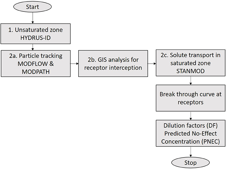
Figure 1. Workflow of the proposed methodology.
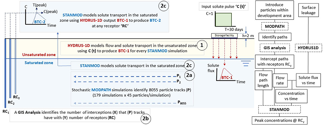
Figure 2. Conceptual diagram of proposed hybrid modelling approach.
Modelling flow and solute transport in the unsaturated zone was carried out using HYDRUS-1D (Šimunek et al., 2016). This one-dimensional numerical model couples transient water flow with reactive solute transport by solving the following governing differential equation:
where C is solute concentration in the liquid phase (M/L3, where M and L are mass and length units, respectively), S is solute concentration in the adsorbed phase (M/L3), D is the dispersion coefficient (L2/T, where T is a time unit), θ is the volumetric water content (L3/L3), v is the pore-water velocity (L/T), ρ is the soil bulk density (M/L3), μl and μs are first-order decay coefficients for degradation of the solute in the liquid and adsorbed phases, respectively (1/T), x and t represent space and time scales, respectively. We assume dispersion D is related to the water velocity v through the dispersivity λ (L) where D = λv. Previous applications of HYDRUS-1D to chemical transport associated with unconventional gas chemicals have demonstrated the versatility of the code to deal with single chemicals as well as multiple chemicals involved in parent-daughter decay reactions with each chemical having different first-order decay coefficients and adsorption parameters (Mallants et al., 2017b).
Details regarding the numerical solution scheme for Eq. 1 are available from Šimunek et al. (2016). Solution of Eq. 1 involves solving first Richard's equation for unsaturated flow with hydraulic properties for each soil horizon. In this study, the van Genuchten (1980)-Mualem (1976) water retention and unsaturated hydraulic conductivity relationships were used, which includes the following parameters: the residual (θs) and saturated (θr) water content, curve-shape parameters α and n, and the saturated hydraulic conductivity, KS.
Solution of Eq. 1 also requires initial and boundary conditions (IC and BC, respectively) for solving the water flow equation. The IC for soil pressure head for the entire flow domain was set to a slight negative pressure of −10 cm (close to saturation). The lower BC was assumed to be a constant pressure head of zero that represents the water table, whereas the upper BC was a mixed head/flux BC (pressure head = 2 m for 30 days representing a temporarily compromised liner, followed by a zero-flux boundary). For solute transport, the IC considered initial concentration equal to zero (solute-free soil profile). The solute flux BC involved contaminated water escaping a leaky storage pond for a duration of 30 days with a unit solute concentration (C = 1); see C(t) in Figure 2.
The output of the HYDRUS-1D simulation is a solute breakthrough curve (BTC). Since flow rates and other transport parameters in the unsaturated soil and saturated groundwater zones differ, these processes were decoupled and solved separately. The solute flux vs. time at the groundwater table (BTC-1 in Figure 2) defined solute delivery to the aquifer, which then became an input to the subsequent modelling stage in the saturated zone.
Modelling solute transport in the saturated zone was carried out using an explicit analytical solution for the ADE under 1-dimensional steady-state flow. The solution requires a priori knowledge of the groundwater flow rate and the length of the flow path. To this end, the modelling exercise involved three steps: (1) particle tracking analysis identified potential flow paths and the associated flow rate along each path (encircled “2a” Figure 2); (2) a GIS spatial analysis determined which of these potential paths did intercept a groundwater dependent receptor based on a site-specific receptor map; this identified the actual length of that path from source to asset (encircled “2b” Figure 2); and (3) the analytical 1-D ADE model generated a breakthrough curve “BTC-2” at relevant receptors RC (encircled “2c” Figure 2). These three steps are discussed in greater detail in the following sections.
This step involves the use of a groundwater flow model and particle tracking analysis to identify the potential flow paths and travel velocities. In this study we used the MODFLOW and MODPATH codes, respectively for flow and particle track simulation.
A spatial analysis involved the identification of particle tracks that would be intercepted by a series of receptors (water bores, surface water bodies, drains and water courses). Once such a particle track was identified, the distance between the source (i.e., gas well) and the receptor (e.g., water bore represented as a point object) was recorded to provide estimates of travel time based on average particle velocity (derived from the particle tracking analysis). For water courses and surface water bodies that are represented as line or surface features, the Euclidian distance from a gas well location to the nearest vertex of a receptor intercepting a particle track line was recorded. Pairs of travel distances and arrival times were obtained for each source-receptor combination, which is required to calculate solute concentrations at the receptor point by solving Eq. 2.
The governing differential equation for 1-dimensional, advective-dispersive solute transport with first order degradation under steady-state flow conditions in a homogenous aquifer is given by:
where ν (=J/η) is the average pore-water velocity and J is Darcy flux (L/T), η is the effective porosity (-), D is dispersion in groundwater (L2/T), and μ is first-order decay coefficient accounting for chemical degradation in groundwater (we assume degradation in liquid (μl) and adsorbed phases (μs) occurs at the same rate, hence can be represented by a single parameter (μ)). R is the retardation factor given by:
where ρb is bulk density (M/L3), Kd is liquid-solid partition coefficient (L3/M), and η is as defined previously.
The non-dimensional flux-averaged concentration (normalised with respect to inlet concentration) is given by van Genuchten et al. (2012):
where c is non-dimensional concentration as a function of non-dimensional space (X) and time (T), which are defined as:
where x is dimensional space, L is the length of the flow domain, v is the average pore water velocity (water flux divided by the water content), and t is dimensional time.
P is the Peclet number given by:
where D is the coefficient of groundwater dispersion.
The CXTFIT code implemented in the software package STANMOD (Šimunek et al., 2009a), provided the explicit analytical solution to Eq. 2. Solute transport parameters were sampled from the parameter ranges listed in Table 1. The output of solute transport modelling is a breakthrough curve (“BTC-2”) at each receptor location RC that has intercepted a particle flow path (marked “2c” in Figure 2). The peak concentration and the time at which it occurred were then recorded for each BTC.
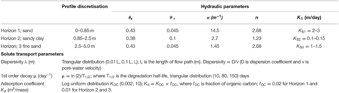
Table 1. Profile layers, hydraulic, and solute transport parameters (m is length units, metre).
As hydraulic and solute transport parameters are highly uncertain, a probabilistic modelling approach was adopted where the uncertainty associated with input parameters was accounted for and results presented as probability distributions that quantify the likelihood of given chemical concentration in the aquifer being reached or exceeded. Stochasticity implemented with a 1D approach can also be viewed as a way of representing heterogeneity in flow paths due to hydrogeological heterogeneity (Toride et al., 1995; Jacques et al., 1997; Vanderborght et al., 2006). Three-dimensional flow and (particularly) solute transport models on the other hand, are associated with long simulation times, and therefore they are not readily conducive to stochastic modelling. Hence, for reasons of efficiency, the 1D hybrid approach was preferred. It is worth noting that because horizontal and vertical transverse dispersion effects were not accounted for in the current 1D models, this means that the analysis is conservative.
As flow and transport processes in the unsaturated and saturated zones were modelled separately using two different approaches and simulation tools, the relevant models were loosely coupled to maintain a quasi-continuous flow path across the unsaturated and saturated zones and making sure fluxes at the bottom of the unsaturated zone were input to the saturated zone simulations. The stochastic modelling process for the saturated zone was carried out as follows:
1. Particle tracking involved the release of 45 particles within the vicinity of the gas well site to identify plausible flow paths within the regional MODFLOW model flow domain. The particle tracking was undertaken in a Monte Carlo analysis with 179 runs.
2. A GIS analysis identified groundwater dependent receptors (groundwater wells and water courses) that may potentially intercept these flow paths, and hence defined their lengths. The average flow rate along each path was calculated from travel times derived from MODPATH.
A Python script was developed to link the unsaturated zone model HYDRUS-1D to the 1D saturated zone solute transport model CXTFIT to predict the peak concentration at receptors that intercepted the flow paths; the script includes the following steps (steps 1–2 relate to the unsaturated zone and steps 3–4 relate to the saturated zone):
1. Select random parameter values for the unsaturated flow and transport model HYDRUS-1D for the following parameters: saturated hydraulic conductivity (KS), liquid-solid partition coefficient (Kd), dispersivity (λ), and first-order degradation coefficient (μ).
2. HYDRUS-1D was executed to define solute breakthrough at the groundwater table (see BTC-1 in Figure 2) for each parameter set. A simulation period of 100 days was sufficient to capture the entire shape of the BTC for the shallow soils of the study area.
3. A source-to-receptor flow path with its characteristic length and flow velocity was randomly selected (derived from the spatial analysis). The solute flux from the previous step was normalised by the unique flow rate of the selected path to yield an input BTC (concentration vs. time) to CXTFIT.
4. Random parameter values were selected for CXTFIT, they include the retardation factor (R), the groundwater dispersion coefficient (D), and first-order degradation coefficient (μ) for the saturated zone. Execution of CXTFIT defines solute breakthrough at receptors (see BTC-2 in Figure 2);
5. The Python code analyses BTC-2 and records the peak concentration and time at which it occurs, marked C(peak) and T(peak) in Figure 2.
6. The steps 1–5 are repeated 1,000 times.
The methodology was implemented in an area with existing conventional gas exploitation in the South East South Australian Otway Basin, near Penola (Figure 3A). New developments are underway including the drilling of several conventional gas wells to depths between 3000 and 4500 m to secure gas production for the area (Beach Energy Limited, 2019). The case study area extends 36 km in an east-western direction and 42 km in a north-southern direction with the towns of Penola in the north and Kalangadoo in the south. The region is characterised by a limestone geology and relatively flat topography with sandy soils (Jacobs, 2016). It has a Mediterranean climate with warm dry summers and cold wet winters, also known as “dry-summer subtropical” Csb based on the Köppen Climate Classification climate classification (South East NRM Board, 2010). Rainfall in the region ranges between 480 and 780 mm/y and potential evapotranspiration ranges from 890 to 1160 mm/year (BOM, 2019). Predominant land uses include dryland grazing, irrigated pasture and viticulture, softwood and hardwood forestry and native vegetation (Jacobs, 2016).
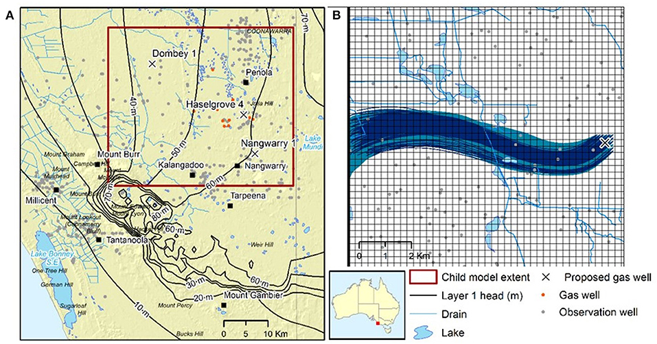
Figure 3. (A) Case study location, child model domain, water features, gas wells, and hydraulic heads in the Tertiary Limestone Aquifer; (B) particle flow paths.
Two major aquifers underlie this region, the unconfined Tertiary Limestone Aquifer (TLA) and the confined Tertiary Confined Sands Aquifer (TCSA). Regional groundwater flows from east to west following the topography (see head contours in the TLA, Figure 3A). Karstic limestone geology characterises the shallow TLA and is extensively used for irrigated agriculture, stock and domestic and other uses (Jacobs, 2016).
Depth to groundwater ranges from <5 m in the south-west plains, to more than 20 m in the north east highlands (Doble et al., 2017). As a result, large parts of the area have poor natural drainage features and have historically been waterlogged. A vast network of agricultural drains was constructed between 1949 and 1972 to artificially lower the groundwater level to facilitate agriculture. A large number of lakes and wetlands are present in this region, many of which are fed by groundwater inflows.
Petroleum and conventional gas wells have been developed in the region around Penola since 1987 with the commercialisation of the Katnook and then the Ladbroke Grove fields. Gas wells have been recently built and/or proposed for this region, including Nagwarry 1, Haselgrove 4, and Dombey 1 wells; these three well locations are cross marked in Figure 3A with only the latter considered in this study.
The 5 m soil profile (the unsaturated zone) for the Dombey 1 gas well site was represented by a three-layer model with each soil horizon having unique hydraulic properties (Table 1). Soil hydraulic properties including water retention parameters and saturated hydraulic conductivity were derived from the HYDRUS-1D soil catalogue (Carsel and Parrish, 1988).
For solute transport modelling, advection-dispersion and reaction parameters used are listed in Table 1. Reference or best estimate parameters for dispersivity λ is one tenth of the travel distance (0.1 × L), which is rule of thumb often applied if no local data on dispersivity is available. The first-order degradation constant μ is based on a chemical half-life of 80 days. This value is based on half-lives (T1/2) of several drilling chemicals such as hexahydro-1,3,5-tris(2-hydroxyethyl)-sym-triazine (T1/2 = 12.2 days), 2-amino ethanol (T1/2 = 30 days), Xanthan gum (T1/2 = 150 days), and carboxymethyl sodium cellulose salt (T1/2 = 280 days). The liquid-solid partition coefficient Kd was derived from KOC values (octanol-water partition coefficient) for the drilling chemical hexahydro-1,3,5-tris (2-hydroxyethyl)-sym-triazine (KOC = 10 and 0.002).
Parameters considered in the stochastic simulations are Ks, λ, μ, and Kd (Table 1). Dispersivity was assigned a triangular distribution with minimum, middle, and maximum values of 0.01 × L, 0.1 × L, and L, respectively. A triangular distribution was also used for the first-order degradation constant μ, i.e., derived from minimum and maximum chemical half-lives of 10 and 150 days, respectively. For KOC a log-uniform distribution was used, with KOC varying between 0.002 and 10.
A regional MODFLOW groundwater flow and MODPATH particle tracking model (Harbaugh, 2005; Pollock, 2012) was developed to identify the likely flow paths between the development area and groundwater-dependent receptors across the study area. Previous groundwater models of the study area include the Wattle Range groundwater model (Wood, 2017), and the South East regional water balance model that was developed in 2014 (Morgan et al., 2015). The former model was developed to model forestry impacts in the Gambier Limestone aquifer and does not incorporate the Tertiary Confined Aquifer. The latter is a regional water balance model that covers an area of 42,000 km2 and includes the study area at the coarse scale of 1 × 1 km grid cells. In this study, a child model was developed with a finer spatial resolution of 250 × 250 m based on the regional water balance model and covering a smaller area that encompasses the gas well-considered in this study. The child groundwater model was developed based on the hydro-stratigraphy and parameterisation of the Wattle Range groundwater model (Wood, 2017) and the Kingston calibration of the South East regional water balance model (Morgan et al., 2015; Wood and Pierce, 2015). FloPy, a python interface for MODFLOW (Bakker et al., 2016), was used to develop the model. The FloPy interface allows partial automation of the model set up and ensures transparency and reproducibility in modelling (Ince et al., 2012; Hutton et al., 2016).
The flow domain was conceptualised as a three-layer system, comprising of an unconfined aquifer (Tertiary Limestone Aquifer), an aquitard (Upper Tertiary Aquitard) and a confined aquifer (Tertiary Confined Sand Aquifer). The model run included a 49-year history matching period from May 1970 to May 2019. Six-monthly stress periods allowed groundwater extraction to vary between summer when irrigation extraction is high, and winter when extraction is very low. Each stress period comprised 10 timesteps. One-second DEM data, upscaled to the 250 m cell size, was used to accurately represent the topography enabling the modelling of surface-groundwater interactions that are important processes in this shallow groundwater environment. Base elevations for Layers 1–3 were adopted from the South-East regional groundwater model.
The South East Regional Water Balance Model was used to generate the following features of the child model:
(i) General head boundary conditions along all four sides of the child model;
(ii) Recharge rates based on the MODFLOW recharge package;
(iii) Groundwater pumping rates through use of the MODFLOW WEL package. The extraction rates were aggregated temporally to the 6-monthly stress period of the child model.
The MODFLOW drain package was used to represent the agricultural drains. A DEM based on LiDAR data flown for the region in 2011 (Wood and Way, 2011) was used to obtain the land surface and the drain locations and the base elevation was defined to be one metre below the land surface. This relative drain depth was consistent with that of the LIDAR data.
The uncertain parameters most relevant in the context of the particle tracking analysis of this study comprised horizontal and vertical hydraulic conductivity, specific yield and specific storage of the two aquifers and intervening aquitard, and the drain conductance. These properties were represented in the calibration and uncertainty analysis by using pilot points as a spatial parameterisation device. Model calibration and uncertainty analysis for the model was carried out using the recently developed PEST-IES utility (White, 2018). The method employed by PEST-IES enables starting from a prior ensemble of parameter realisations, sampled from a uniform distribution between the lower and upper bounds, to evaluate the calibration objective function and progressively derive the posterior parameter set that provides best match with observation data. In this study PEST-IES (White, 2018) was used to do the history matching of model simulated groundwater head to observations for the period between 1970 and 2019. A total of 2,694 adjustable parameters were used, and 5,761 observations of groundwater head were available within the child model area. Initial values of the parameters were specified based on values obtained from the regional groundwater model (Wood, 2017). The calibration and uncertainty analysis of the model using the PEST-IES software resulted in the generation of 500 equally likely realisations of the model parameters that can calibrate the model to the observations. A random subset of 200 realisations were then used in the particle tracking analysis using MODPATH to simulate the advective transport travel times and distances in the aquifer. A total of 179 runs successfully completed the forward particle tracking runs and thus used in the current work. The remaining 21 runs failed due to numerical and/or computational inconsistencies.
For a surface-based contamination associated with the drilling of a gas well, the particle track starts from the groundwater table and identifies potential flow paths and travel times in the surficial aquifer. It was assumed that the starting point of the particle tracks could be located anywhere within the model cell containing the gas well or any cell adjacent to it. For the Dombey 1 gas well area (Figure 3A), forty-five particles were assigned uniformly to a total of nine grid cells each 250 × 250 m2 as demonstrated in Figure 3B. Particle tracking was undertaken in this study using MODPATH 7.
The HYDRUS-1D stochastic simulations produced one thousand breakthrough curves, which describe the solute flux at the lower boundary of the flow domain (at the groundwater table). One thousand simulations were confirmed to be sufficient to capture the proposed parameter uncertainties, for example, increasing the number of simulations from 900 to 1000 resulted only in 0.39% and 0.66% changes in the mean and standard deviation of the peak solute flux, respectively. The general shape of the solute BTC at the bottom boundary (the water table) is shown in Figure 4 (the BTC shown in Figure 4 was obtained by averaging the 1,000 simulated BTCs). During the first 30 days of the simulation and while the storage facility was allowing water to seep through the liner, the solute flux continued to increase until it reached after around 20 days a constant water flux at a constant solute concentration equal to that at the inlet (unity). The average steady-state water flux was 0.28 m/day. After water infiltration ceased (t > 30 days), the soil profile continued to drain freely until an insignificant solute flux was reached at 100 days (at which the water flux was 0.002 m/day). Each of the 1,000 BTCs was approximated by 10 linear segments and explicitly used as input to CXTFIT for modelling solute transport in the aquifer. Note that the area under the BTC shown in Figure 4 represents the total solute mass delivered to the aquifer, which is referred to hereafter as the cumulative solute flux. Note that the output of the stochastic simulations can be interpreted as a representation of lateral heterogeneity in soil horizons whereby each stochastic realisation represents a unique soil profile with a different set of hydraulic parameters at a particular point.
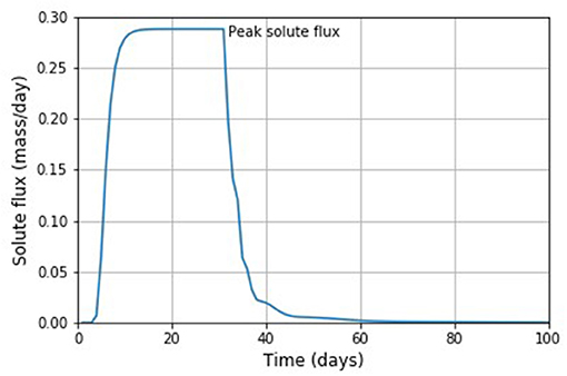
Figure 4. Average breakthrough curve (BTC) derived from 1,000 stochastic HYDRUS-1D simulations.
Figure 5A shows the distribution of the peak solute fluxes obtained from the 1000 simulations, which range from 0.17 to 0.37 with a median of 0.28 (mass units/day per unit of spatial area). Figure 5B shows the distribution of the cumulative solute flux delivered to the aquifer at the conclusion of each of the thousand 100-day simulations; values range from 4.78 to 10.67 with a median of 7.84 (mass units per unit area of spatial area). Figure 5C demonstrates that the peak and cumulative solute fluxes are almost perfectly correlated (see R2 on the figure), hence, the sensitivity analyses presented hereafter were restricted to the peak solute flux as the cumulative solute flux yielded identical trends.
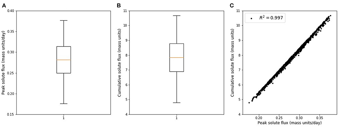
Figure 5. Box plot of peak (A), and cumulative (B) solute fluxes; scatter plot of peak vs. cumulative solute fluxes (C). Fluxes obtained from stochastic HYDRUS-1D simulations. Box plot shows median (amber line), interquartile range (box), and range of all values (whiskers).
The stochastic simulations have shown a wide range of solute fluxes varying by a factor of 2.23 (10.67/4.78). To understand which model parameters were responsible for this variation, scatterplots were developed showing if and how the peak solute flux was influenced by the six parameters that were treated as stochastic variables during the 1000 HYDRUS-1D simulations. These parameters included the saturated hydraulic conductivities of the three soil horizons (KS1, KS2, and KS3), the first-order decay constant μ (derived from the chemical half-life), the adsorption coefficient Kd, and the dispersivity λ. Figures 6A,C show that the solute flux is not sensitive to the hydraulic conductivities of the top and bottom soil horizons as evident by the random distribution of the 1,000 data points. The effect of varying the hydraulic conductivity was dominated by the middle soil layer, which acted as an impeding throttle layer controlling water and solute fluxes (Figure 6B). This was confirmed by monitoring the pressure head at the interface between horizons one and two, which indicated a perched water table due to the low permeability of the second horizon (results not shown here). There is a strong positive correlation between the solute flux and KS2: a high KS2 value means the leaking fluid will reach the groundwater table much sooner than for a small KS2 value. Faster transport also means less degradation will occur in the unsaturated zone, therefore delivers more solute mass to the groundwater. Note that the solid yellow line in Figure 6B represents a special case without solute degradation, which clearly shows the sole influence of the conductivity.
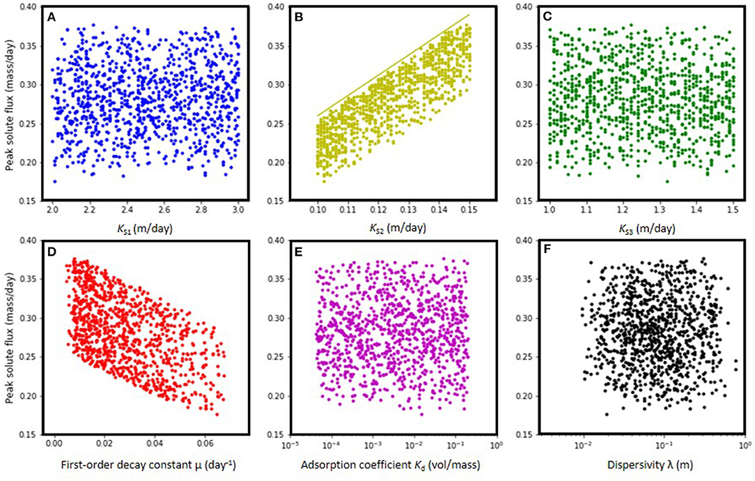
Figure 6. Cross-plots for six parameters KS1 (A), KS2 (B), KS3 (C), μ (D), Kd (E), and λ (F) used in stochastic HYDRUS-1D simulations.
Figure 6D shows the influence of the first-order degradation constant (based on half-life) on the peak solute flux. The negative correlation results from little chemical degradation occurring when the half-life value is large (or small first-order degradation constant), while conversely chemicals with a short half-life (large first-order degradation constant) will display considerable decay thus reducing concentration and hence fluxes. Note that the wide range of peak solute fluxes at any one value of KS2 (Figure 6B) can mostly be attributed to variations in the first-order degradation constant. Figure 6E shows that the peak solute flux is not sensitive to changes in the adsorption coefficient Kd; note that sorption was considered to depend on organic carbon and given the small fraction (0.02 for horizon 1 and 0.01 for horizon 2 and 3), the Kd varied between 5 × 10⁻⁴ and 0.2 L/kg, albeit small values causing only little solute retardation. Hence, the impact of the adsorption coefficient was insignificant especially when compared to the significant effects of KS2 and μ. Similarly, variation in dispersivity had a relatively insignificant effect on peak solute concentration (Figure 6F).
To test whether or not the numerical solution has converged and met the stringent stability criteria associated with solute transport, mass balance information and convergence parameters were extracted from the relevant HYDRUS-1D output files following the completion of each simulation, they are summarised in Figure 7.
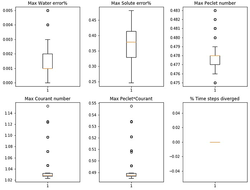
Figure 7. Run time information demonstrating convergence of stochastic HYDRUS-1D simulations.
Specifically, HYDRUS-1D reports the following mass balance information and stability criteria throughout the simulation (at user-defined time steps), note recommended stability criteria in brackets: relative error in water mass balance (<5%), relative error in solute mass balance (<5%), Peclet number (≤2), Courant number (≤1), and the product of Peclet and Courant numbers (≤2) (Šimunek et al., 2009b). Based on these criteria, the convergence of the simulation was assessed resulting in a convergence flag (True or False). The summary convergence criteria (Figure 7) show very small water and solute mass balance errors with Peclet and Courant numbers much below their threshold values. These results show that all simulations are numerically accurate.
The Monte Carlo particle tracking simulation conducted within the regional MODFLOW model provided 179 completed model runs resulting in a total of 8055 particle tracks (45 × 179 referred to as “P” number of particle tracks in Figure 2). Spatial analysis was undertaken to identify the primary risk receptors—groundwater bores and water courses that were intercepted by the particle tracks within a 10 m vicinity. The nearest receptors within a 2-km distance class were all groundwater bores, hence the groundwater bores were deemed to be the risk receptors in the solute transport analyses. The spatial analysis identified the number of particle tracks (X) that intercepted (Y) number of receptors (refer to description of X and Y in Figure 2). The particle tracks are shown in Figure 3B, which also shows the 14 bores that were intercepted within a 10 km range (see grey dots encircled in yellow; note that the total interceptions within the 12 km range was 16 bores).
Figure 8A shows the distribution of flow path lengths between the source (gas well location) and the interception point at groundwater-dependent receptors. There were 16 groundwater bores that were intercepted by the particle tracks from the Dombey 1 gas well (referred to as “RCy,” in Figure 2). Out of the 8055 tracks, 1476 tracks (referred to as “X” in Figure 2) have intercepted the 16 receptors (referred to as “Y” in Figure 2) thus resulting in an interception probability of 18.34%; the interception probability and the number of receptors (Y) for individual 2000-m distance intervals are listed at the upper x-axis of Figure 8A. This means that each receptor was intercepted multiple times with particles that travelled through tracks of varying lengths at various flow rates as a result of changing parameters in the MODPATH simulations. For example, the three bores located within 0–2000 m were intercepted n = 545 times thus resulting in an interception probability of 6.77% (545/8055); interceptions for each of the six flow path length intervals are listed in Figure 8A (n is the cumulative frequency of interception for each length interval).
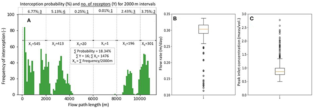
Figure 8. (A) Distribution of particle tracks that intercepted groundwater-dependent assets and probability of interception for 2000 m intervals; (B) Distribution of average groundwater flow rates along flow paths; (C) Distribution of solute inlet concentration into aquifer.
The distribution of flow rates along each of the particle tracks is shown in Figure 8B with a median flow rate of 0.3 m/day. Note that the data underpinning Figures 8A,B were stored as pairs of length and flow rate along each track. For each of the CXTFIT stochastic simulations, a random travel distance was sampled from the distribution shown in Figure 8A and used along with its paired flow rate to model solute breakthrough. A time series (similar to that shown in Figure 4) was randomly selected from the stochastic HYDRUS-1D outputs and used as the input solute flux time series; the latter was normalised by the sampled flow rate to result in an “inlet” solute BTC entering the aquifer (input into CXTFIT simulation). Figure 8C shows the distribution of the peak “inlet” concentrations in the aquifer, which is obtained by dividing solute flux data of Figure 5A by flow data of Figure 8B. Remembering that the inlet solute concentration at the source was equal to unity, one can note in Figure 8C that in some simulations, the concentration is higher than the source, this occurs when the flow rate in the aquifer is much smaller than that in the unsaturated zone thus yielding a concentration effect, conversely, if the flow rate is higher a dilution effect occurs at the source.
CXTFIT was run to solve the 1D ADE and define a BTC along each of the identified flow paths that intercepted one or more of the identified receptors; the BTC was then analysed to identify the peak solute concentration at receptor locations. Solute transport parameters were randomly sampled from the ranges listed in Table 1. Figure 9A shows the peak concentrations at receptors that have intercepted particle flow paths for particles that travelled up to 1000 m (as beyond 1000 m the dilution was large enough to reduce concentrations to negligible levels). Multiple peak concentrations are displayed at a given flow path length or travel distance (the nearest located at 166 m from the source, Figure 9A). The distribution of flow path lengths (x-axis of Figure 9A) corresponds to that identified by the spatial analysis shown in Figure 8A, with a cut-off at 1000 m. The effect of the longer flow paths on peak concentration is evident, with a consistent decline in peak concentration as the travel length increases (the dotted in Figure 9A highlights a declining maximum peak concentration as travel distance increases). The overall highest peak concentration was 9% of the input unit concentration at the source, which occurred at the receptor closest to the source. The wide range of concentrations extending more than seven orders of magnitude at any flow path length is mostly attributed to the effect of solute degradation. Figure 9B shows the probability of exceeding a given peak concentration, for instance in 83% of the stochastic simulations the peak concentration was <1% of the input unit concentration at the source. The peak concentrations for all flow path lengths reported in Figure 9 are influenced by the first-order degradation coefficient, aquifer dispersivity and flow rate. As flow rate dictates residence time, this parameter has a direct effect on solute degradation through its influence on residence time. Hence, given this interdependence, parameter sensitivity was investigated one-at-a-time whereby one parameter was varied, and the others kept constant.
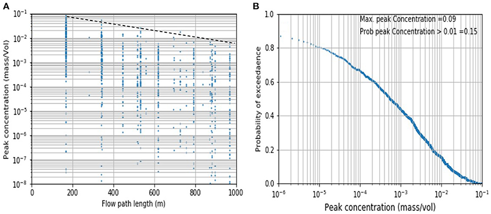
Figure 9. (A) Peak concentrations vs. flow path lengths within 1000 m range; (B) Probability of exceeding peak concentrations.
Figure 10A shows the sensitivity of peak concentrations to the first-order degradation coefficient while dispersivity was kept constant; note that the discrete lines along which the sensitivity varies having significantly different slopes correspond to the discrete flow path lengths shown in Figure 9A (two of which are labelled; L = 166 m and 341 m). Steeper slopes correspond to longer flow path lengths and hence longer residence times, with the latter leading to larger solute degradation. In order to isolate the effect of variable flow rates, the same simulations were repeated while fixing the flow rate to the median value of 0.3 m/day. The resulting peak concentrations were identical with the exception of the encircled points in Figure 10A disappearing as these points correspond to the 5th percentile of the simulated flow rates, the lower end associated with larger residence times.
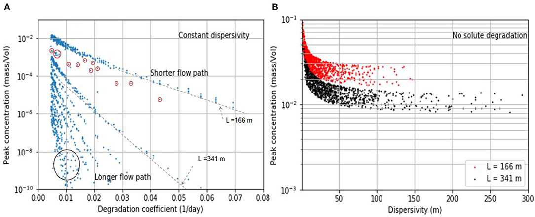
Figure 10. (A) Peak concentration sensitivity to first-order degradation constant; (B) Peak concentration sensitivity to dispersivity.
Figure 10B shows the sensitivity of peak concentrations to dispersivity for two flow path lengths with no solute degradation. Excluding degradation and considering unique flow path lengths was deemed necessary in order to filter out the dispersion effect. Figure 10B shows that a higher dispersivity leads to lower peak concentrations, with the effect diminishing for dispersivity values higher than 0.3L (note flattening trend in Figure 10B). The variations in peak concentration for a given dispersivity value is attributed to variable input concentrations and flow rates (the data represents a band not a line).
The solute transport modelling presented here resulted in identifying the most influential parameters affecting natural attenuation that solutes may undergo in the unsaturated and saturated zones. The analyses identified peak concentrations (Cpeak) at explicit receptor locations (Figure 9A) for a wide range of hydraulic and solute transport parameters resulting from a unit input concentration (Ci) at the source. The outcome of this research highlights the importance of site-specific characterisation. This includes a detailed knowledge of soil profiles within areas of potential contamination; in this work, the effect of a throttle layer on solute fluxes was highlighted, conversely, one can obviously postulate that preferential paths would have the opposite effect of accelerating the arrival of solutes to the groundwater system. Solute degradation has a profound effect on concentration, hence, the interaction between soils and specific chemicals needs to be thoroughly understood. Finally, and though obvious, the larger the distance between the contamination source and a point of environmental significance is, the higher the dilution and the lower the risk is. However, this highlights the importance of identifying groundwater flow paths and flow rates along these paths, hence a thorough understanding of the groundwater flow system is warranted.
The degree of natural attenuation is quantified by the ratio Ci/Cpeak, which reflects the dilution level of a solute, termed herein the Dilution Factor (DF). Since the input concentration used in this work was unity, then the DF is simply the reciprocal of the peak concentration. The hybrid modelling approach for computing DFs across the saturated and unsaturated zones has potential applicability in informing management or regulatory decisions. For example, it can be used to infer buffer distances for attaining safe levels of natural attenuation for potable water quality or to avoid aquatic toxicity for targetorganisms.
Natural attenuation is impacted by many factors including the length of the flow path with longer paths associated with larger dilution while longer residence times result in greater biochemical degradation and mass removal through adsorption processes. For these results to be useful in practical applications, the solute transport calculations were re-analysed to derive 50th (median) and 95th percentile DFs at each receptor location; this was done for every unique flow path length shown as a discrete vertical line in Figure 9A. Figure 11 shows that the DFs increase exponentially as a function of travel distance (straight lines on a semi-logarithmic scale). Simple analytic expressions were derived for the 50th (median) and 95th percentile DF and are shown in Figure 11. An example application using these expressions is discussed herein.
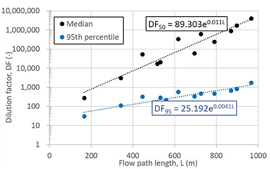
Figure 11. Median (DF50) and 95th percentile dilution factors (DF95) vs. flow path length.
A variety of chemicals are associated with developments for and production of natural gas (drilling, waste, and production chemicals such as condensates) (DEM, 2019). Such chemicals are used in different concentrations and have different toxicity levels (Tran-Dinh et al., 2019). As a chemical naturally attenuates, its concentration decreases until it reaches an acceptable value for a specific ecotoxicity endpoint (e.g., fish or daphnia); this is termed the predicted no-effect concentration (PNEC) (DoE, 2017). The minimum dilution factor required to achieve this concentration (DFmin) is the ratio of the input concentration at source to the predicted no-effect concentration (Ci/PNEC). Having identified mathematical expressions that relate DF to travel path length, one can then define the minimum flow path length (L) required to achieve the minimum dilution factor DFmin. For example, the DFmin for citric acid1 (PNEC = 15.3 mg/L for chronic endpoint for Daphnia) (DoE, 2017) is equal to 186 given a source concentration of 2853 mg/L (concentration in drilling fluid) (Beach Energy Limited, 2019). To achieve this DF value, the minimal buffers required are 67 and 488 m such that the 50th and 95th percentile peak concentrations are not exceeded, respectively.
This analysis can help regulators identify safe buffer zones around gas development areas. Similarly, it can also aid in managing concentrations at the source by defining a maximum concentration to satisfy a minimum dilution factor for a certain buffer distance. Note that the dilution and dispersion in the saturated and unsaturated zone were calculated with one-dimensional models. These models underestimate dispersion due to their 1-dimensional nature, therefore the results reported here are deemed to be conservative.
The hybrid modelling approach adopted in this study has a regional focus with the objective of simulating DFs for a broad range of plausible parameter combinations and considering the groundwater-dependent receptors across the region. While this approach is generic and can be applied for computing DFs for such applications, the model scales and parameters should be tailored to suit the individual application, source-receptor combinations and chemical species of interest.
This work examined the plausible pathways for groundwater contamination risk from surface handling of chemicals associated with conventional gas development in the southeast South Australia considering the gas well at the Dombey 1 site as an example. A hypothetical chemical leak scenario considered a compromised storage facility of fluids that led to leakage of contaminants into soil and groundwater for a duration of 30 days. A stochastic modelling methodology was adopted whereby flow and transport in the unsaturated and saturated zones were approximated by 1-dimensional models. The stochastic modelling involved, firstly, coupled flow and solute transport in the unsaturated zone using HYDRUS-1D, and secondly, 1D solute transport during steady-state groundwater flow using the analytical model CXTFIT. Groundwater flow rates and travel distances were obtained from particle tracking using a 3D MODPATH model. A spatial analysis was carried out to identify travel paths for implementing the CXTFIT model that intercepted known groundwater-dependent receptors in the area. Despite the fact that this novel approach integrates many models, it is more conducive to stochasticity as individual model run times are small. The method is applicable for flow and transport modelling problems in the context of contamination risk assessment for valuable receptors where reliable quantification of the risk is important.
The stochastic HYDRUS-1D simulations have shown that solute loads may vary by more than two-folds thus highlighting the importance of explicit vadose zone transport modelling when assessing the environmental impacts of surface spills. Sensitivity analyses of six HYDRUS-1D parameters have shown that peak solute concentration and total solute load delivered to the aquifer were mainly sensitive to the first-order degradation coefficient and the saturated hydraulic conductivity of the middle low-conductivity soil horizons that acted as a throttle layer. The other parameters tested, i.e., adsorption coefficient Kd, dispersivity λ, and saturated hydraulic conductivity of the top and bottom horizon were found to be less influential.
The stochastic simulations considered probable ranges for soil and aquifer hydraulic and chemical reaction parameters. Calculations showed a significant reduction in solute concentration at the receptor relative to its source concentration, with an overall maximum peak concentration of 9% of the source concentration. Stochastic simulations showed that 87% of the simulations had concentrations of <1% of the source concentration.
It was shown that a 1D stream tube approach was adequate for modelling solute transport along the curvilinear contaminant trajectories in the aquifer. This allowed the coupling a 1D numerical vadose-zone model to an analytical solver of the advective-dispersive equation of solute transport in the aquifer to stochastically assess contamination risks associated with gas developments. Spatial analyses of the contaminant trajectories and the actual groundwater-dependent receptors identified all paths that can potentially intercept a receptor. We presented an example were buffer distances were derived for attaining safe levels of natural attenuation for potable water quality or to avoid aquatic toxicity for target organisms.
The scope of this study was to provide a cost-effective screening analysis to evaluate groundwater contamination risks at receptor locations for a broad range of soil, aquifer and chemical characteristics of the study site and plausible scenarios of contamination events. Results provide information to regulators about residual risks when standard management and clean up procedures are accounted for.
The original contributions presented in the study are included in the article/Supplementary Material, further inquiries can be directed to the corresponding author.
DR, JS, and DM conceptualised the method. DR led the manuscript writing with contributions from DM and JS. DR completed the analytical modelling and risk assessment. JS and DG undertook the particle tracking analysis. RD development the groundwater flow model used for particle tracking analysis. TP undertook the parallel model runs on the cluster computing facility and contributed to model uncertainty analysis. All authors contributed to the article and approved the submitted version.
This research was funded by CSIRO's Gas Industry Social and Environmental Research Alliance (GISERA). GISERA is a collaboration between CSIRO, Commonwealth and State Governments and Industry established to undertake publicly reported independent research. The purpose of GISERA is for CSIRO to provide quality assured scientific research and information to communities living in gas development regions focusing on social and environmental topics including groundwater, surface water, biodiversity, land management, marine environment, human health impacts and socio-economic impacts.
The authors declare that the research was conducted in the absence of any commercial or financial relationships that could be construed as a potential conflict of interest.
All claims expressed in this article are solely those of the authors and do not necessarily represent those of their affiliated organizations, or those of the publisher, the editors and the reviewers. Any product that may be evaluated in this article, or claim that may be made by its manufacturer, is not guaranteed or endorsed by the publisher.
The Supplementary Material for this article can be found online at: https://www.frontiersin.org/articles/10.3389/frwa.2021.799738/full#supplementary-material
Supplementary Figure 1. Part of the MODFLOW-MT3D model domain, flow boundary conditions and solute sources (cells 1–50), and sinks (extraction wells).
Supplementary Figure 2. Contours of steady-state pressure head distribution and particle path lines for two extraction scenarios; a solute BTC was derived using 1D analytical solution for each path line shown.
Supplementary Figure 3. Particle flow path lengths and flow rates for two extraction scenarios (identical extraction rates but different well locations).
Supplementary Figure 4. Comparison of breakthrough curves derived with the hybrid approach (1D analytical ADE using particle tracking velocities) and MT3D.
1. ^Alternative chemical name: 1,2,3-Propanetricarboxylic acid, 2-hydroxy- (CAS # 77-92-9).
Bakker, M., Post, V., Langevin, C. D., Hughes, J. D., White, J. T., Starn, J. J., et al. (2016). Scripting MODFLOW model development using Python and FloPy. Groundwater 54, 733–739. doi: 10.1111/gwat.12413
Beach Energy Limited (2017). Haselgrove 3 Disclosure Report 7040180_02-1. Adelaide, SA: Beach Energy Ltd.
Beach Energy Limited (2019). Environmental Impact Report, Drilling, Completion and Well Production Testing in the Otway Basin, South Australia. Available online at: https://sarigbasis.pir.sa.gov.au/WebtopEw/ws/samref/sarig1/image/DDD/PGER000082019 (accessed March 20, 2021).
BOM (2019). Gridded long term mean annual rainfall for Australia. Commonwealth of Australia. Melbourne VIC: Bureau of Meteorology. Available online at: http://www.bom.gov.au/jsp/ncc/climate_averages/rainfall/index.jsp (accessed July 10, 2019.
Brantley, S. L., Yoxtheimer, D., Arjmand, S., Grieve, P., Vidic, R., Pollak, J., et al. (2014). Water resource impacts during unconventional shale gas development: the Pennsylvania experience. Int. J. Coal Geol. 126, 140–156. doi: 10.1016/j.coal.2013.12.017
Carsel, R. F., and Parrish, R. S. (1988). Developing joint probability distributions of soil water retention characteristics. Water Resour. Res. 24, 755–769. doi: 10.1029/WR024i005p00755
Cousins, I. T., Vestergren, R., Wang, Z., Scheringer, M., and McLachlan, M. S. (2016). The precautionary principle and chemicals management: the example of perfluoroalkyl acids in groundwater. Environ. Int. 94, 331–340. doi: 10.1016/j.envint.2016.04.044
DEM (2019). Assessment of Beach Energy's Proposed Onshore Otway Basin Petroleum Production and Processing Activities. Adelaide, SA: Department of Energy and Mining (DEM), South Australian Government.
Doble, R. C., Pickett, T., Crosbie, R. S., Morgan, L. K., Turnadge, C., and Davies, P. J. (2017). Emulation of recharge and evapotranspiration processes in shallow groundwater systems. J. Hydrol. 555, 894–908. doi: 10.1016/j.jhydrol.2017.10.065
DoE (2017). Environmental Risks Associated With Surface Handling of Chemicals Used in Coal Seam Gas Extraction in Australia, Project Report Appendices A, B, C, D, F, and G Prepared by the Chemicals and Biotechnology Assessments Section (CBAS) in the Department of the Environment and Energy as Part of the National Assessment of Chemicals Associated with Coal Seam Gas Extraction in Australia, Commonwealth of Australia, Canberra. Canberra, ACT: DoE.
Harbaugh, A. W. (2005). MODFLOW-2005: The U.S. Geological Survey Modular Ground-Water Model–The Ground-Water Flow Process. Book 6: Modelling Techniques, Section A. Groundwater. Reston, VA: USGS.
Hutton, C., Wagener, T., Freer, J., Han, D., Duffy, C., and Arheimer, B. (2016). Most computational hydrology is not reproducible, so is it really science? Water Resour. Res. 52, 7548–7555. doi: 10.1002/2016WR019285
Ince, D. C., Hatton, L., and Graham-Cumming, J. (2012). The case for open computer programs. Nature 482, 485–488. doi: 10.1038/nature10836
Jackson, R. B., Vengosh, A., Darrah, T. H., Warner, N. R., Down, A., Poreda, R. J., et al. (2013). Increased stray gas abundance in a subset of drinking water wells near Marcellus shale gas extraction. Proc. Natl. Acad. Sci. U.S.A. 110, 11250–11255. doi: 10.1073/pnas.1221635110
Jacobs (2016). Hydrogeological Risk Assessment—Unconventional Gas Well—South East. Brisbane, QLD: Department of State Development.
Jacques, D., Vanderborght, J., Mallants, D., Kim, D.-J., Vereecken, H., and Feyen, J. (1997). Comparison of three stream tube models predicting field-scale solute transport. Hydrol. Earth Syst. Sci. 1, 873–893. doi: 10.5194/hess-1-873-1997
Lechtenböhmer, S., Altmann, M., Capito, S., Matra, Z., Weindorf, W., and Zittel, W. (2011). Impacts of Shale Gas and Shale Oil Extraction on the Environment and on Human Health. Wuppertal Institute for Climate, Environment and Energy and Ludwig-Bölkow-Systemtechnik GmbH, Study Requested by the European Parliament's Committee on Environment, Public Health and Food Safety, IP/A/ENVI/ST/2011–07 Wuppertal: Wuppertal Institute.
Mallants, D., Apte, S., Kear, J., Turnadge, C., Janardhanan, S., Gonzalez, D., et al. (2017a). Deeper Groundwater Hazard Screening Research. Canberra, ACT: Commonwealth Scientific and Industrial Research Organisation (CSIRO).
Mallants, D., Bekele, E., Schmid, W., Miotlinski, K., Taylor, A., Gerke, K., et al. (2020). A Generic method for predicting environmental concentrations of hydraulic fracturing chemicals in soil and shallow groundwater. Water 12:941. doi: 10.3390/w12040941
Mallants, D., Jeffrey, R., Zhang, X., Wu, B., Kear, J., Chen, Z., et al. (2018). Review of plausible chemical migration pathways in Australian coal seam gas basins. Int. J. Coal Geol. 195, 280–303. doi: 10.1016/j.coal.2018.06.002
Mallants, D., Šimunek, J., and Genuchten, M. T., Jacques, D. (2017b). Simulating the fate and transport of coal seam gas chemicals in variably-saturated soils using HYDRUS. Water 9:385. doi: 10.3390/w9060385
Meyer, P. D., Valocchi, A. J., and Eheart, J. W. (1994). Monitoring network design to provide initial detection of groundwater contamination. Water Resour. Res. 30, 2647–2659. doi: 10.1029/94WR00872
Morgan, L. K., Harrington, N., Werner, A. D., Hutson, J., and Woods, J. (2015). South East Regional Water Balance Project—Phase 2, Development of a Regional Groundwater Flow Model. Goyder Institute for Water Research Technical Report Series No. 15/38. Adelaide, SA: Goyder Institute, 138.
Mualem, Y. (1976). A new model for predicting the hydraulic conductivity of unsaturated porous media. Water Resour. Res. 12, 513–522.
Oppel, J., Broll, G., Löffler, D., Meller, M., Römbke, J., and Ternes, T, (2004). Leaching behaviour of pharmaceuticals in soil-testing-systems: a part of an environmental risk assessment for groundwater protection. Sci. Total Environ. 328, 265–273. doi: 10.1016/j.scitotenv.2004.02.004
Pollock, D. (2012). User Guide for MODPATH Version 6—A Particle-Tracking Model for MODFLOW. Chapter 41 of Section A, Groundwater Book 6, Modeling Techniques and Methods 6–A41. Reston, VA: USGS.
Prommer, H., Rathi, B., Donn, M., Siade, A., Wendling, L., Martens, E., et al. (2016). Geochemical Response to Reinjection. Final Report. Canberra, ACT: CSIRO. Available online at: https://gisera.csiro.au/wp-content/uploads/2018/03/Water-1-Final-Report.pdf (accessed March 20, 2021).
Šimunek, J., Sejna, M., Saito, H., Sakai, M., and van Genuchten, M. T. (2009a). The HYDRUS-1D Software Package for Simulating the Movement of Water, Heat, and Multiple Solutes in Variably Saturated Media, Version 4.08; HYDRUS Software Series 3. Riverside, CA: Department of Environmental Sciences, University of California Riverside, 330.
Šimunek, J., van Genuchten M, T., and Šejna, M. (2016). Recent developments and applications of the HYDRUS computer software packages. Vadose Zone J. 15:25. doi: 10.2136/vzj2016.04.0033
Šimunek, J., van Genuchten, M.T., Šejna, M., and Toride, N., Leij, F.J. (2009b). Studio of Analytical Models for Solving the Convective-Dispersive Equation (STANMOD). Available online at: www.hydrus3d.com (accessed March 03, 2021).
South East NRM Board (2010). Natural Resource Management Plan, Part One: Regional Description. Adelaide, SA; South East Natural Resource Management Board, Government of South Australia.
Sreekanth, J., Cui, T., Pickett, T., Rassam, D., Gilfedder, M., and Barrett, D. (2018). Probabilistic modelling and uncertainty analysis of flux and water balance changes in a regional aquifer system due to coal seam gas development. Sci. Total Environ. 634, 1246–1258. doi: 10.1016/j.scitotenv.2018.04.123
Sreekanth, J., Moore, C., and Wolf, L. (2015). Estimation of optimal groundwater substitution volumes using a distributed parameter groundwater model and prediction uncertainty analysis. Water Resour. Manag. 29, 3663–3679. doi: 10.1007/s11269-015-1022-y
Toride, N., Leij, F. J., and van Genuchten, M. Th. (1995). The CXTFIT Code for Estimating Transport Parameters From Laboratory or Field Tracer Experiments. Research Report No. 137. Riverside, CA: Salinity Laboratory, Agricultural Research Service, US Department of Agriculture.
Torres, L., Yadav, O. P., and Khan E. (2016). A review on risk assessment techniques for hydraulic fracturing water and produced water management implemented in onshore unconventional oil and gas production. Sci Total Enviro. 539, 478–493. doi: 10.1016/j.scitotenv.2015.09.030
Tran-Dinh, N., Vergara, T. J., Schinteie, R., Mariani, C., and Midgley, D. J. (2019). Microbial Degradation of Chemical Compounds Used in Onshore Gas Production in the SE of South Australia. Canberra, ACT: CSIRO.
US EPA (2016). Hydraulic Fracturing for Oil and Gas: Impacts From the Hydraulic Fracturing Water Cycle on Drinking Water Resources in the United States, EPA/600/R-16/236Fa. Washington, DC: Office of Research and Development.
van Genuchten, M. T. (1980). A closed-form equation for predicting the hydraulic conductivity of unsaturated soils. Soil Sci. Soc. Am. J. 44, 892–898. doi: 10.2136/sssaj1980.03615995004400050002x
van Genuchten, M. T., Šimůnek, J., Leij, F. J., Toride, N., and Šejna, M. (2012). STANMOD: Model Use, Calibration, and Validation. Trans ASABE. 55, 1353–1366.
Vanderborght, J., Kasteel, R., and Vereecken, H. (2006). Stochastic continuum transport equations for field-scale solute transport: overview of theoretical and experimental results. Vadose Zone J. 5, 184–203. doi: 10.2136/vzj2005.0024
White, J. T. (2018). A model-independent iterative ensemble smoother for efficient history-matching and uncertainty quantification in very high dimensions. Environ. Model. Softw. 109, 191–201. doi: 10.1016/j.envsoft.2018.06.009
Wood, C. (2017). Lower Limestone Coast Forest Water Accounting Groundwater Model, DEWNR Technical Report 2017/14. Adelaide, SA: Government of South Australia, Department of Environment, Water and Natural Resources.
Wood, C., and Pierce, D. (2015). South East Confined Aquifer Modelling Investigations—Kingston Groundwater Management Area, DEWNR Technical Report 2015/48. Adelaide, SA: Government of South Australia, Through Department of Environment, Water and Natural Resources.
Wood, G., and Way, D. (2011). Development of the Technical Basis for a Regional Flow Management Strategy for the South East of South Australia, DFW Report 2011/21. Adelaide, SA: Government of South Australia, Through Department for Water.
Keywords: risk assessment, contaminant transport, vadose zone modelling, python, MODFLOW, MT3D, advective-dispersive transport, groundwater
Citation: Rassam D, Sreekanth J, Mallants D, Gonzalez D, Doble R and Pickett T (2022) Stochastic Assessment of Groundwater Contamination Risks From Onshore Gas Development Using Computationally Efficient Analytical and Numerical Transport Models. Front. Water 3:799738. doi: 10.3389/frwa.2021.799738
Received: 22 October 2021; Accepted: 13 December 2021;
Published: 11 January 2022.
Edited by:
Yoram Rubin, University of California, Berkeley, United StatesCopyright © 2022 Rassam, Sreekanth, Mallants, Gonzalez, Doble and Pickett. This is an open-access article distributed under the terms of the Creative Commons Attribution License (CC BY). The use, distribution or reproduction in other forums is permitted, provided the original author(s) and the copyright owner(s) are credited and that the original publication in this journal is cited, in accordance with accepted academic practice. No use, distribution or reproduction is permitted which does not comply with these terms.
*Correspondence: David Rassam, ZGF2aWQucmFzc2FtQGNzaXJvLmF1; J. Sreekanth, U3JlZWthbnRoLkphbmFyZGhhbmFuQGNzaXJvLmF1
Disclaimer: All claims expressed in this article are solely those of the authors and do not necessarily represent those of their affiliated organizations, or those of the publisher, the editors and the reviewers. Any product that may be evaluated in this article or claim that may be made by its manufacturer is not guaranteed or endorsed by the publisher.
Research integrity at Frontiers
Learn more about the work of our research integrity team to safeguard the quality of each article we publish.