 A. O. Opere
 Ruth Waswa
- Department of Earth and Atmospheric Sciences, University of Nairobi, Nairobi, Kenya
Narok County in Kenya is the home to the Maasai Mara Game Reserve, which offers important habitats for a great variety of wild animals, hence, a hub for tourist attraction, earning the county and country an extra income through revenue collection. The Mau Forest Complex in the north is a source of major rivers including the Mara River and a water catchment tower that supports other regions as well. Many rivers present in the region support several activities and livelihood to the people in the area. The study examined how the quantity of surface water resources varied under the different climate change scenarios, and the sensitivity of the region to a changing climate. Several datasets used in this study were collated from different sources and included hydro–meteorological data, Digital Elevation Model (DEM), and Coordinated Regional Downscaling Experiment (CORDEX) climate projections. The WEAP (Water Evaluation and Planning) model was applied using the rainfall–runoff (soil moisture method) approach to compute runoff generated with climate data as input. All the calculations were done on a monthly time step from the current year account to the last year of the scenario. Calibration of the model proceeded using the PEST tool within the WEAP interface. The goodness of fit was evaluated using the coefficient of determination (R2), percentage bias (PBIAS), and Nash–Sutcliffe efficiency (NSE) criterion. From the tests, it was clear that WEAP performed well in simulating stream flows. The coefficient of determination (R2) was greater than the threshold R2 > 0.5 in both periods, i.e., 0.83 and 0.97 for calibration and validation periods, respectively, for the monthly flows. A 25-year mean monthly average was chosen with two time slices (2006–2030 and 2031–2055), which were compared against the baseline (1981–2000). There will be a general decrease in water quantity in the region in both scenarios: −30% by 2030 and −23.45% by 2055. In comparison, RCP4.5 and Scenario3 (+2.5°C, +10% P) were higher than RCP8.5 and Scenario 2 respectively. There was also a clear indication that the region was highly sensitive to a perturbation in climate from the synthetic scenarios. A change in either rainfall or temperature (or both) could lead to an impact on the amount of surface water yields.
Introduction
Water is a crucial natural resource and necessary for the support of life on earth. Retrogression of the environment and climate change has posed challenges in the management and allocation of available water resources (Wang et al., 2005; Leal Filho, 2015; Okyereh et al., 2019). However, the freshwaters of the world are under increasing pressure, and many still lack access to adequate water to meet their basic needs (Cap-Net, 2006).
Population growth increases economic activities, causes a change in standards of living, and eventually results in the depletion of limited freshwater resources. A report by the World Bank in 2005 estimated a larger population of people to be living under stressful conditions of absolute water scarcity and is expected to worsen by the year 2025. Climate and demographic changes are such factors that can effectuate the exhaustion of water resources and also lead to high demands of energy (Asaf et al., 2007; Kadner et al., 2008; Aloysius et al., 2015; Khadra, 2019). This, in turn, presents tough decisions especially to policymakers and water managers, and the only option to curb the shortages is to factor in the balance between supply and demand (Conway, 2009).
The African continent has an area of about 30 million square kilometers. It has several valuable resources such as natural forests, minerals, wildlife, and diversity in biological existence (Kotchecheeva and Singh, 2000).
Climate change impacts can be greatly felt by the communities around the African continent and the ecosystem, depending on the geographical positioning of these countries, population, and their capacity to adapt and mitigate the effects of changes in climate (Urama and Ozor, 2010). According to Leal Filho (2015), Africa is the most vulnerable continent to climate and climate variability. The rate of warming patterns is alarming, subjecting the continent to high variability of rainfall in space and time. Some parts of the continent are experiencing extensive drought conditions, with others severely affected by heavy rains and floods resulting in loss of livelihoods to people in these places (Nelson, 2004; Luo et al., 2005; Trenberth et al., 2005; Verdin et al., 2005).
The changing patterns of climate, which include the variable trends in precipitation and temperatures are inimical on the socioeconomic sector of Kenya. Illegal logging, poor farming practices, and encroachment into forest lands have hastened the degradation of these lands, and as such, the forest cover in Kenya has fallen from 12% in the 1960s to 2% at the present state. This has greatly affected the main water towers, which are the major sources of water for consumption in both rural and urban settings (NCCRS, 2010).
Narok County in Kenya is among the crucial counties in the country for the achievement of the economic pillar of Kenya's Vision 2030. It supports several activities including livestock and crop farming, and an ecosystem to the Maasai Mara Game Reserve, which offers important habitats for a great variety of wild animals, hence, a hub for tourist attraction, earning the county and country extra income through revenue collection. The Mau Forest Complex in the north is a source of major rivers including the Mara River and a water catchment tower that supports other regions as well. Many rivers present in the region support several activities and livelihood to the people in the area. The main objective of this study was to assess the impacts of climate change on surface water resources in Narok County using the WEAP modeling tool. The study examined how the quantity of surface water resources varied under the different climate change scenarios and the sensitivity of the region to a changing climate. Based on the coefficient of determination (R2) and other statistics used in this study, the results showed that the WEAP model was able to simulate the stream flow patterns fairly well.
Characteristics of the Study Area
The County of Narok in Kenya is one of the 47 counties in Kenya and is located south of the equator between latitude 0°50′S and 1°50′S and longitude 35°28′E and 36°25′E, located in the Rift Valley region of Kenya (see Figure 1 below). The area spans from near the equator to the southern border of Kenya–Tanzania with an area of 17,944.1 km2. The main administrative town is Narok town, which is also the center of all economic activities. Kenya National Bureau of Statistics (KNBS, 2019) census report estimates a population of 1,149,379 for the region.
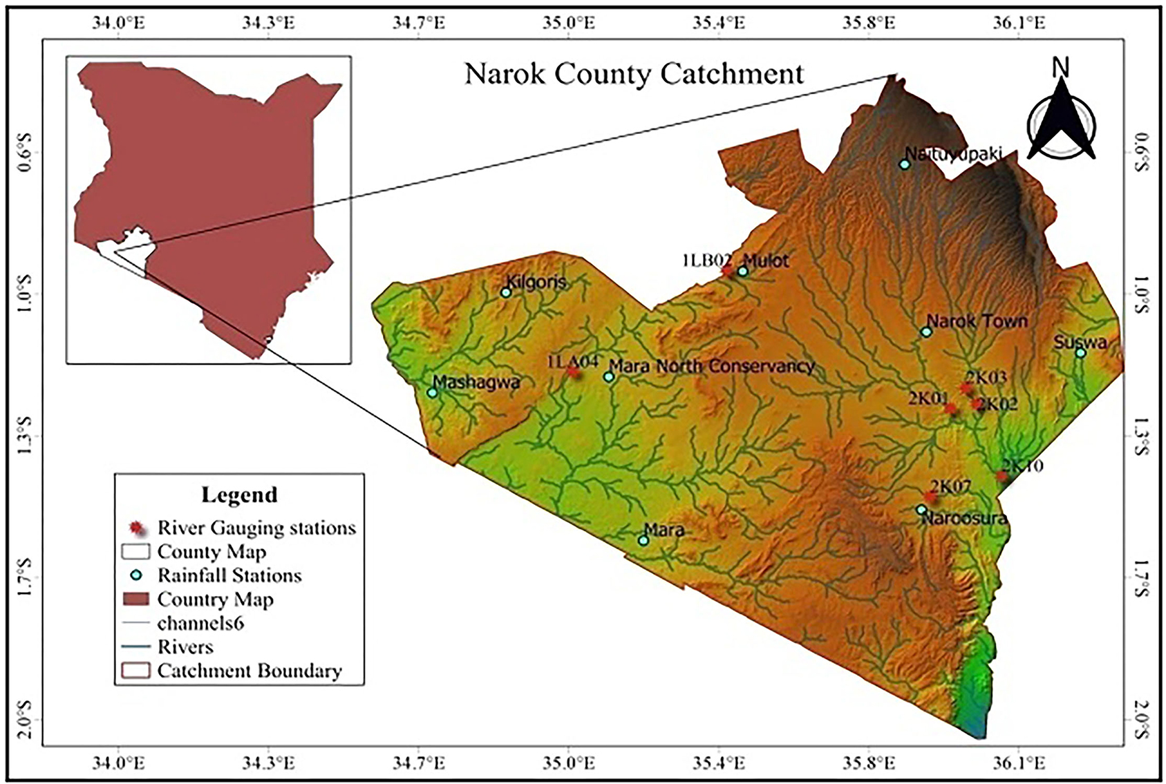
Figure 1. Location of Narok County catchment with RGSs.
Temperature
Temperature ranges from about 22°C in the Southeastern part of Kalema in February–March to 13.3°C in the Northern parts of Kisiriri during July. However, the region records an average temperature of about 18°C. Generally, the coolest month is July, while February–April and October–December are the warmest months in almost all stations in the study area.
Rainfall
The region has two main wet seasons; March–May and September–November, though some stations in this region exhibit a trimodal rainfall pattern within June–August. The mean monthly rainfall ranges from about 12 mm in July to about 191 mm in April. Rainfall totals vary from 650 to 1,300 mm annually.
Hydrology
Three main rivers drain the region; Mara, Ewaso Ng'iro, and Migori rivers. Ewaso Ng'iro river has its headwaters high in the Mau rising to the north of Olokurto and flows southeastward to the edge of Nguruman into the Rift Valley. This river is fed by several tributaries such as Narok and Siyabei rivers which also have their headwaters from the Mau region. Mara River has its source near that of Ewaso Ng'iro in the Mau and flows southeastward in the Siria escarpment to form the “Mara Triangle,” then south toward Tanzania, and then westwards into Lake Victoria near Musoma. Migori River rises near Abossi and drains the Transmara plateau, and flows south then west to join river Kuja near the Tanzania border before flowing into Lake Victoria.
However, Sondu River and Ewaso Kedong are the two peripheral rivers in the region that are important to the ecosystem. The Mau region in the north mainly drains into lakes Nakuru, Naivasha, and Elementaita. All the permanent rivers in the area derive their headwaters from the Mau region.
Materials and Methods
There were several categories of data that were used in this study, which were collated from different sources which included; hydro-meteorological data, digital elevation model (DEM) data, and CORDEX climate projections. Hydrological data was obtained from the Water Management Authority (WMA), meteorological data from the Kenya Meteorological Department (KMD) which was substituted with Climate Hazard Group Infrared Precipitation with Stations (CHIRPS) and Fifth Assessment Report (ERA5) datasets. CHIRPS datasets were obtained from the IGAD Climate Prediction and Application Center (ICPAC) data repository while the ERA5 dataset was obtained from the Climate Explorer webpage (http://climexp.knmi.nl/) (Accessed on February 5, 2020). Topographical (DEM) data were downloaded from the United States Geological Survey (USGS) webpage (http://srtm.csi.cgiar.org/) (Accessed on February 5, 2020) while the CORDEX outputs were obtained from the WCRP CORDEX domain (https://esgf-data.dkrz.de) (Accessed on March 10, 2020).
The other datasets used in this study were obtained from several downscaling groups such as the United States Regional Climate Model Version 3 (RegCM3); Canadian Regional Climate Model (CRCM); United Kingdom Met Office Hadley Center's Regional Climate Model Version 3 (HadRM3) and IPCC; and were in the native model format grid and projection. The sixth phase of the Coupled Model Intercomparison Project (CMIP6) data is reported either on the native grid of the model or regridded to one or more target grids with data variables generally provided near the center of each grid cell (rather than at the boundaries). For CMIP6, there is a requirement to record both the native grid of the model and the grid of its output (archived in the CMIP6 repository) as a “nominal resolution.” The “nominal resolution” enables users to identify which models are relatively high resolution and have data that might be challenging to download and store locally. These datasets had to be converted and placed into identical horizontal and vertical estimates using bilinear interpolation before any analysis was performed.
Water Evaluation and Planning Model Setup and Modeling Procedure
WEAP is a water demand and supply accounting model (water balance accounting), which provides capabilities for comparing water supplies and demands as well as for forecasting demands.
Unlike most other hydrological models, the WEAP model allows the flexibility of assessing the future water shortages by the integration of demographic and other socioeconomic indicators with a changing climate to come up with the overall impact on water availability. However, the current study has only addressed the impact of a changing climate on water availability.
Application of a WEAP model can support water management potential conflicts arising from competing demands of complex water resource systems that require a holistic approach to address the various components of water management (WEAP, 2015). Using the area of study, the model was set up in the schematic view and the catchment setup included the infiltration channels to the catchment, rivers, and gauges on these rivers. The current account, key assumptions, time steps, and scenarios were also defined. Climate data was loaded onto the catchment including the catchment area and the latitude. Gauged stream flow was also loaded under the supply and resources module. An initial run of the model was done at a selected gauging station on Ewaso Ng'iro River (RGS2K01), to establish if the parameters were correctly loaded, and establish the suitability of the model and prepare it for calibration and validation, in order to improve on the model simulations and reduce any uncertainties. To perform calibration and validation of the model, Ewaso Ng'iro (RGS2K01) was chosen and monthly time steps chosen with a three-step procedure as follows;
(i) Sensitivity analysis
(ii) Parameter calibration
(iii) Model validation
Model Sensitivity Analysis
This was done manually using monthly observed discharge data for the period 1985–1990 from Ewaso Ng'iro RGS (2K01). The model was used to calculate the observed function between the observed and simulated values. Parameters were ranked according to the degree of sensitivity (Van Liew and Veith, 2010; Rwigi, 2014).
Model Calibration and Validation
To appropriately simulate historical observations, the calibration process of parameters was done. Monthly observed stream flow data from 1985 to 1987 at RGS2K01 were used for calibration and 1988 to 1990 used for validation. The PEST tool within the WEAP interface was used in combination with a manual approach. To aid the process of calibration, the PEST tool was used to modify some parameters, while others were manually adjusted. A comparison between the observed and simulated stream flows was used as a criterion to evaluate the model performance based on the following statistics, i.e., coefficient of determination (R2), Nash–Sutcliffe efficiency (NSE), and percentage bias (PBIAS). This study adopted all the three evaluation statistics to assess the performance of the WEAP model before being applied in hydrological modeling (Nash and Sutcliffe, 1970; Rwigi, 2014; Moriasi et al., 2015).
Model Simulations
There are five methods within WEAP to model catchment processes (Azadani, 2012; Seiber and Purkey, 2015): rainfall–runoff (simplified coefficient and soil moisture methods), irrigation demands only method, and plant growth methods that are highly dependent on the purpose of analysis and data availability. This study used the rainfall–runoff (soil moisture method) to compute runoff with climate data as input. All the calculations were done on a monthly time step from the current year account to the last year of the scenario.
The rainfall–runoff or soil moisture method simulates catchment runoff with two soil layers. The upper soil layer simulates runoff, shallow interflow, soil moisture changes, and evapotranspiration. The base flow and soil moisture are simulated in the lower layer. This method is also one dimensional and uses two control volumes (buckets) for a catchment unit. The catchment is classified into sections that represent the soil types and land uses, for j and N sub-catchments, assuming that the climate in that catchment is constant. The mass water balance equation is given by;
where Rdj (mm) is the land cover fraction, Z1, j is the relative storage and is a fraction of effective root zone, Pe is the effective precipitation, which includes snowmelt from snow parks within each watershed, mc is the melt coefficient, PET is the Penman–Monteith crop potential evapotranspiration, kc,j is a fraction for each land cover, ks,j is the root zone saturated conductivity (mm/time), and fj is the portioning fraction (horizontally and vertically) based on the soil type, land cover, and topography. Figure 2 presents the concept of the soil moisture method and the equations involved.
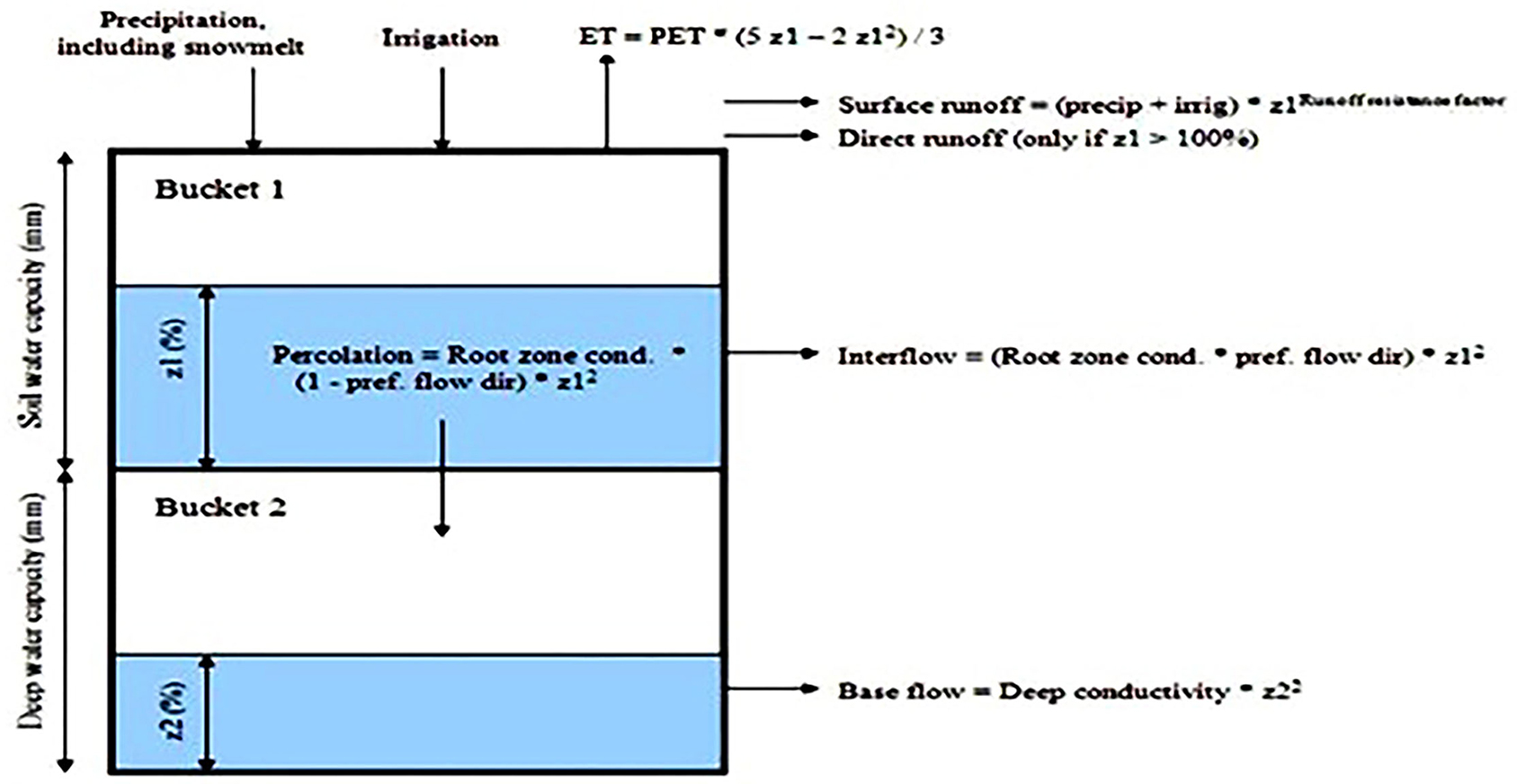
Figure 2. Representation of the soil moisture method and equations (Seiber and Purkey, 2015).
Creation of Synthetic Scenarios
Scenarios mimic the future situations of systems like how well they will respond to various conditions, such as climate change, and thus can be used to assess the impact of climate change and develop climate adaption strategies (Jusoh, 2007; Azadani, 2012). A synthetic scenario approach assists in estimating the amount and extent of climate change by altering a climatic variable to identify the critical threshold, which facilitates the analysis of the sensitivity of a system to climate change (Islam et al., 2005). Synthetic scenarios are created by altering the existing climate conditions (reference year period/current account) and applied to generate future climate scenarios. Typically, they are based on the changes in annual means in both temperature and precipitation from simple adjustment, e.g., ΔT = ± 1°C, ± 2°C, ± 4°C, and ΔP = 0, ± 10%, ± 20%.
Synthetic scenarios were created to investigate how sensitive the hydrological system is to climate change (Oti, 2019). Four scenarios were created to evaluate and compare the potential impacts of climate change in the county, for the period 2021–2055. These included a base (reference) scenario of no change and three hypothetical scenarios of a + 2.5°C temperature increase combined with no change or a change of ± 10% in precipitation applied to historical data from 1981 to 2000, to develop climate change scenarios for further analysis.
Most global circulation models depict an increase in the annual mean temperature projection by (0.8–1.5°C) by 2030, 1.0–2.8°C by 2050, (1.6–2.7°C) by 2060s, and 3°C by 2100, while rainfall will vary from 2–11% by 2060 and 12% by 2100, indicating possible increase (Butterfield, 2009; KNAP, 2016; USAID, 2018; Gebrechorkos et al., 2019; Sagero, 2019).
In this regard, three hypothetical scenarios of a 2.5°C temperature increase combined with a change of ± 10% in precipitation was applied to historical data from 1981 to 2000, to develop climate change scenarios for further analysis as summarized in Table 1 below. A baseline (reference) scenario of no change was also included.
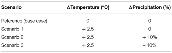
Table 1. Synthetic climate change scenarios.
Impact Assessment
This was done at the county level by analyzing projected stream flows using rainfall and temperature as input data, under two scenarios, RCP4.5 and RCP8.5. The impacts of climate change on stream flows were assessed by comparing the water available (quantity) during the baseline period and future projections, including the scenarios of increased/reduced rainfall and temperature, done at two levels as follows;
(i) Impact of climate change on the quantity of water (water yields) using the GCM scenarios following the RCP4.5 and RCP8.5 pathways.
(ii) Impact of climate change by the use of synthetic scenarios.
Results
Sensitivity analysis was carried out to establish the most appropriate and sensitive parameters for calibration. Table 2 presents the results of sensitivity analysis.
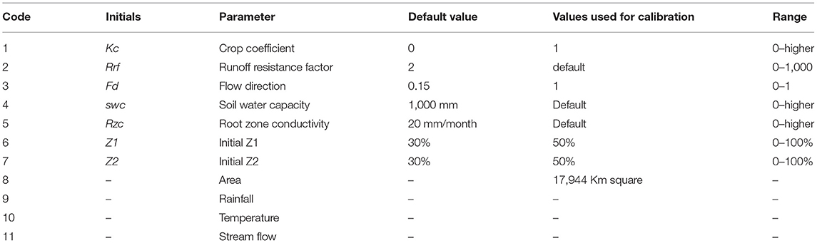
Table 2. Calibration parameters adopted for modeling the stream flow.
The model parameters were ranked according to their sensitivity, starting from the most sensitive parameter to the least, which were also responsible for the stream flow generation in the catchment. Other than the catchment area and mandatory climate parameters, the most sensitive parameter was crop coefficient (Kc) with rank 1, followed by the runoff resistance factor (Rrf) with rank 2, and so on, while the least were Z1 and Z2 as shown in Table 2.
Model Calibration and Validation
This process proceeded by using the PEST tool within the WEAP interface. A time series of observed monthly stream flow and WEAP simulated outputs for both calibration and validation periods, i.e., (1985–1987 and 1988–1990), together with their regression outputs, are shown in Figures 3A,B, 4A,B. The results indicated a strong positive correlation between observed and simulated discharge for Ewaso Ng'iro at RGS 2K01. The value of R2 was 0.83 for the calibration period and R2 = 0.97 for the validation period.
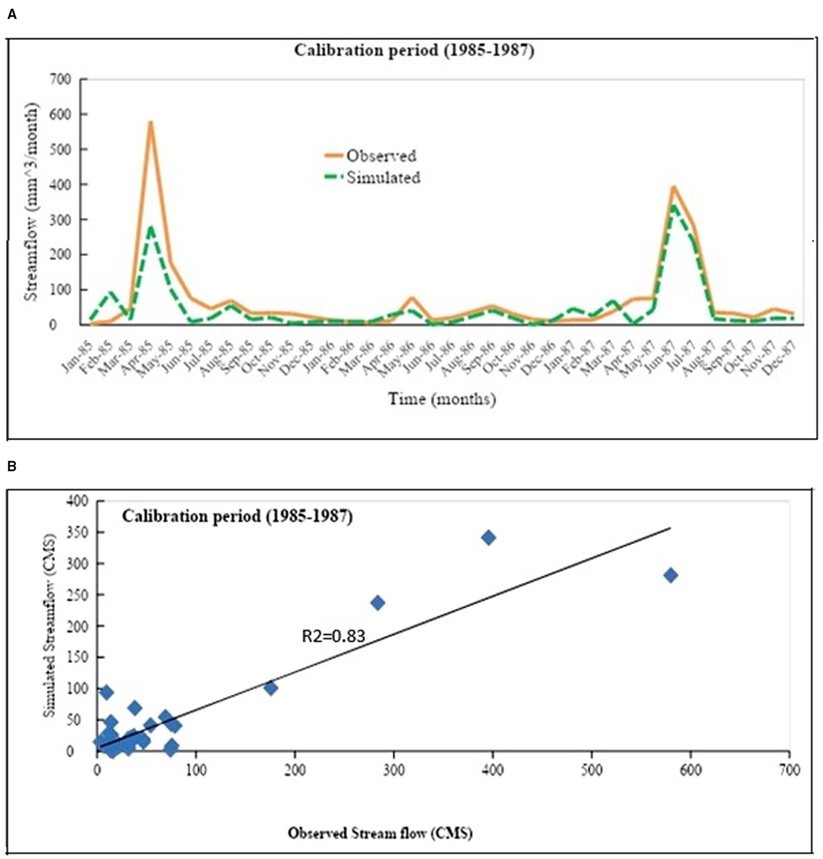
Figure 3. (A) Observed and simulated stream flow during the calibration period at Ewaso Ng'iro (RGS2K01). (B) Regression line during the calibration period at Ewaso Ng'iro (RGS2K01).
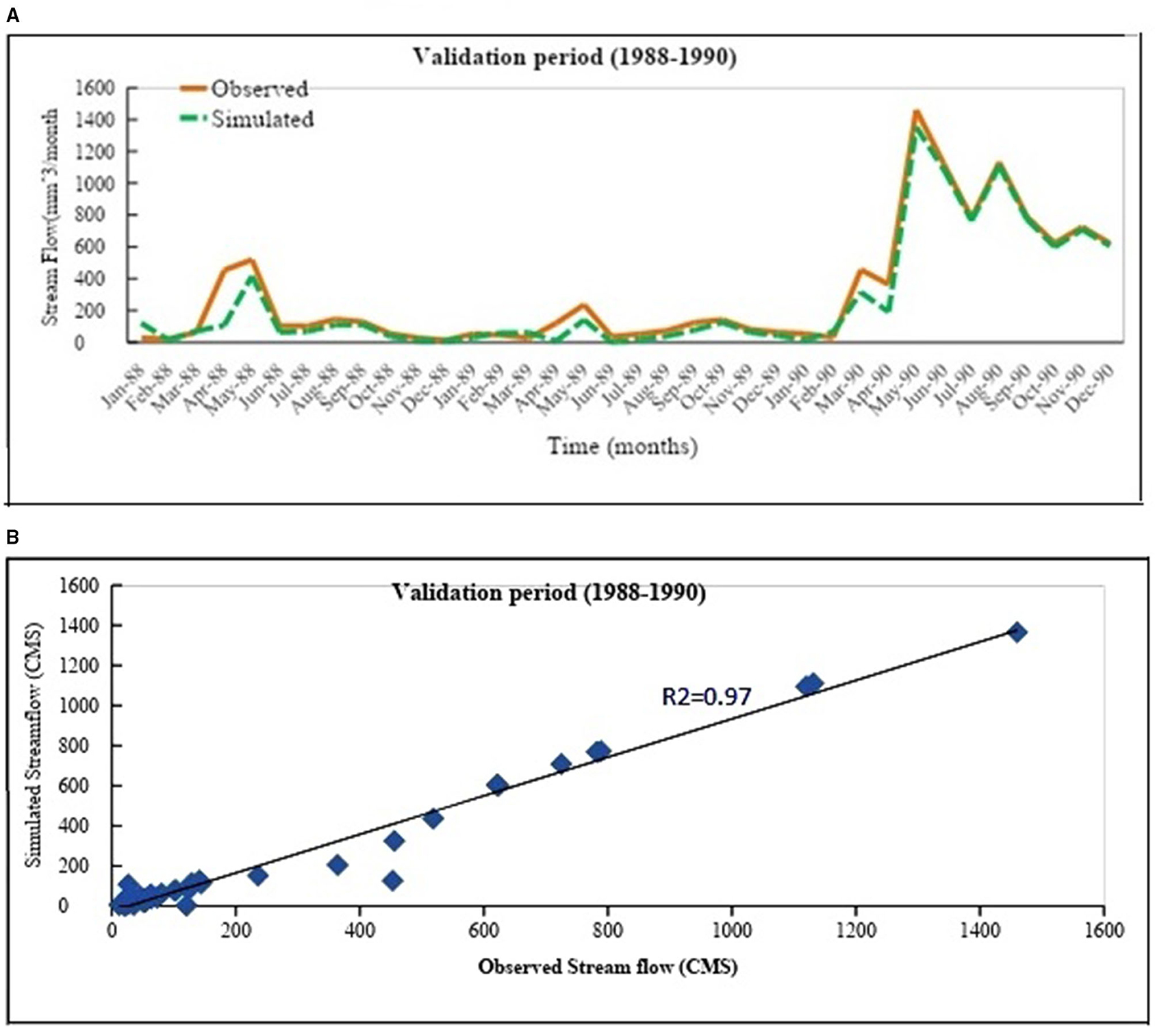
Figure 4. (A) Observed and simulated stream flow during the validation period. (B) Regression line during the validation period at Ewaso Ng'iro (RGS2K01).
The stream flow patterns were well-captured by the model in the calibration and validation periods. However, the model slightly overestimated the flows in the year 1987 in the calibration period and underestimated the peak flows in April in 1985 and 1988 in both periods. The disparity in this observation could have been due to possible water management processes used to address “what if situations;” besides the short period of data used for calibration.
The coefficient of determination (R2) was greater than the threshold R2 >0.5 in both periods, i.e., 0.83 and 0.97 for calibration and validation periods, respectively, for the monthly flows as shown in Figures 3A,B, 4A,B.
The percentage bias (PBIAS) showed the best performance in simulating the stream flows (Table 3). The calibrated and simulated values fell within the acceptable range (± 10% ≤ PBIAS ≤ ± 25%) as suggested by Rwigi (2014) and Moriasi et al. (2015). During the calibration period, the PBIAS value was 22.3% while the validation period had a 12.7% PBIAS.
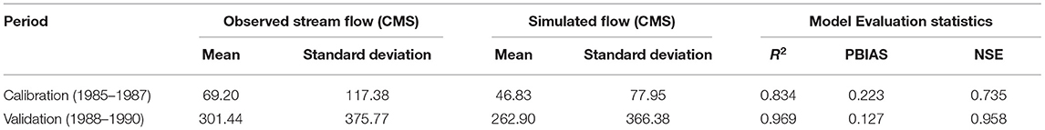
Table 3. Statistics of observed and simulated stream flows for the calibration and validation periods.
The values of NSE in simulating the stream flows were 0.74 during the calibration period and 0.96 during the validation period. These again were within the acceptable range (0.75 < NSE ≤ 1.0) according to Rwigi (2014) and Moriasi et al. (2015).
On the basis of the PBIAS, NSE, and R2 results; it was clear that the model performed well in simulating stream flows.
Stream Flow Projections Under Climate Change Scenarios
WEAP model was used to project stream flows at Ewaso Ng'iro (RGS2K01) under RCP4.5 and RCP8.5 scenarios. A 25-year mean monthly average was chosen with two time slices (2006–2030 and 2031–2055), which were compared against the baseline (1981–2000). An additional time slice (2021–2030) was chosen to represent the projections from the current time to the year 2030. Figure 5A shows the monthly stream flow projections under RCP4.5 against the baseline. There is a likelihood of increased water yields from the months of November–March and also July, in all the time slice periods, except for December for the period 2031–2055. Months currently experiencing low water yields (November, December, January, February, March, and July) will experience higher yields mostly by the year 2030, while those with higher yields will experience a fluctuation by 2055 (April–October) except July. This will be in response to a projected positive increase in rainfall from the baseline period (1981–1990) to the year 2030 and then a slight decrease after the period to the year 2055 under RCP4.5 (Waswa, 2020). The lowest monthly stream flow projected is 102.4 CMS by the year 2030 and 84.9 CMS by the year 2055.
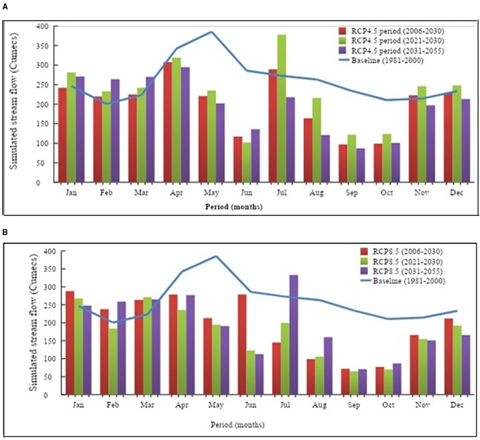
Figure 5. (A) Simulated and baseline mean monthly stream flows for RCP4.5 for Ewaso Ng'iro at RGS2K01. (B) Simulated and baseline mean monthly stream flows for RCP8.5 for Ewaso Ng'iro at RGS2K01.
Figure 5B shows water yields under RCP8.5. However, the model projections under RCP8.5 indicate that by the year 2030, all the months except January and March are projected to remain dry. January–March and July are projected to have increased yields by 2055, which reflects a kind of seasonal shift in the monthly flows before and after 2030. The period 2031–2055 will record the highest amount of discharge in July (306.3 CMS) with a low of 67.9 CMS in September. By 2030, the month of March will have the highest discharge (271 CMS) with the lowest projected to be in September (65 CMS).
From the results, the period 2021–2030 will have a slight increase in water yields in both scenarios, with RCP4.5 recording a higher yield than RCP8.5. January, February, and March are projected to have increased water yields in both periods.
Figure 6 below is a comparison of stream flow projections under scenarios RCP4.5 and RCP8.5. The monthly flow in RCP4.5 is projected to have higher yields than in RCP8.5. The months November–April and July will have higher water yields under RCP4.5.
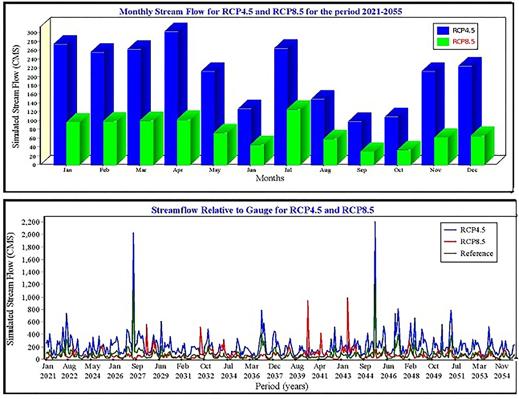
Figure 6. Comparison of monthly and annual stream flow projection under RCP4.5 and RCP8.5.
Projected Stream Flow Patterns Under Synthetic Scenarios
In this case, rainfall and temperature were altered, according to need, in order to simulate stream flow. Four scenarios were created (normal temperature and precipitation, increased temperature alone, increase in temperature and precipitation, and an increase in temperature and reduced rainfall). These scenarios were useful in quantifying water yields and availability for the period 2021–2055. Two time slices were applied: 2021–2030 and 2031–2055 against the baseline 1981–2000.
A change in either precipitation or temperature affects surface runoff directly. Regarding the changes in the climate parameters used in each scenario, four different simulations were obtained with respect to the amount of water yields. Figure 7 shows projected monthly surface runoff for the period 2021–2030 and 2031–2055. The reference scenario is the current account, with normal rainfall and temperature.
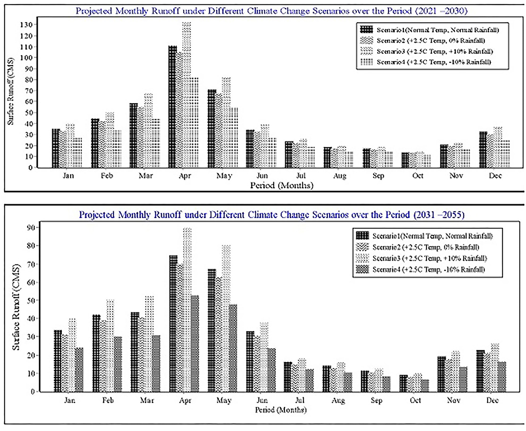
Figure 7. Projected monthly synthetic scenarios over the period 2021–2055.
Figure 8 presents the projection of annual simulated flows from the four scenarios for the two periods (2021–2030 and 2031–2055).
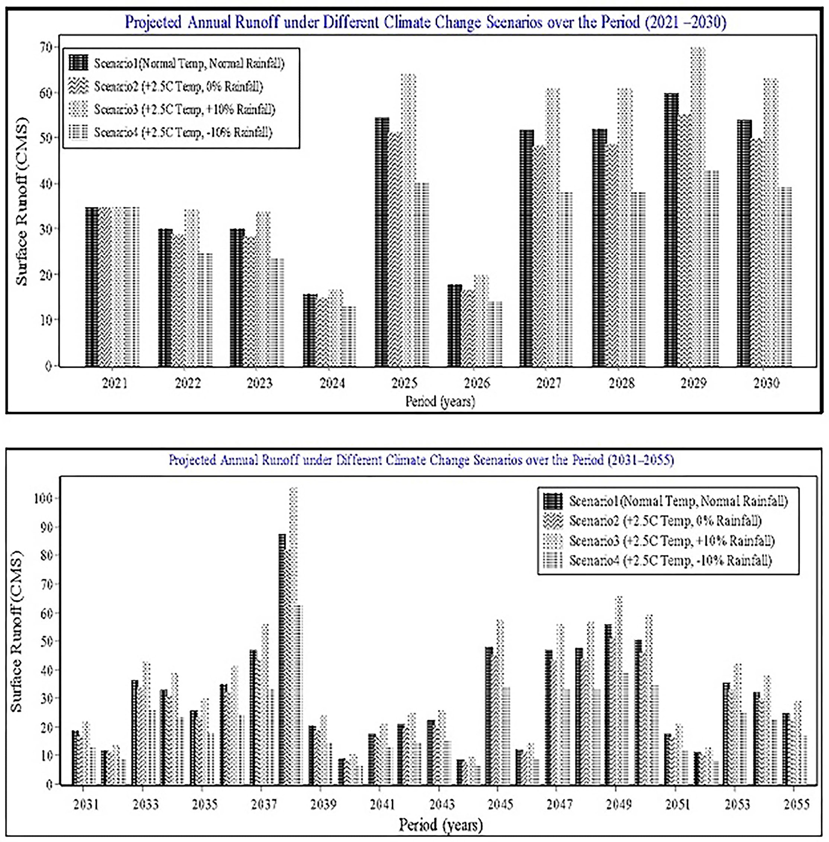
Figure 8. Projected monthly synthetic scenarios over the period 2021–2055.
Discussion
The results show that there is a likelihood of increased water yields from the month of November–March and also July, in all the time slice periods, except for December for the period 2031–2055. Months currently experiencing low water yields (November, December, January, February, March, and July) will experience higher yields mostly by the year 2030, while those with higher yields will experience a fluctuation by 2055 (April–October) except July. Figures 5A,B shows water yields under RCP4.5 and RCP8.5 respectively. By the year 2030, all the months except January and March are projected to remain dry. January–March and July are projected to have increased yields by 2055. The period 2031–2055 will record the highest amount of discharge in July (306.3 CMS) with a low of 67.9 CMS in September. By 2030, the month of March will have the highest discharge (271 CMS) with the lowest projected to be in September (65 CMS). A similar study in the Sondu catchment (Rwigi et al., 2016) noted that there will be increases in monthly rainfall ranging between 9 and 489% over the baseline between September and May, and fall between June and August by between 14 and 24% of the baseline (1991–1990). This is expected to translate into low and high water yields, respectively.
High temperature is most likely to have an impact on water yields due to high rates of evaporation. An increase in temperature and a decrease in rainfall amount could be the reason behind the decrease in water yields in the region in both scenarios. According to the study on the Kenya Water Towers (Mwangi et al., 2020), the projected changes in maximum and minimum temperatures for the three scenarios (RCP2.6, RCP4.5, and RCP8.5) for three future time slices of 2030s, 2050s, and 2070s have shown that almost all areas of the Kenya Water Towers will experience a warming trend. The expected warming extent is greatest during MAM and JJAS seasons, and least during the short rains (OND). The short rains (OND) are projected to increase over most parts of the domain (Mau Forest Complex, Mt. Elgon, and Cherangany Hills) under all the three scenarios (Mwangi et al., 2020). In contrast, the long rains (MAM and JJAS) are projected to decrease over most of the region. The projected annual rainfall shows a tendency to increase over the western and southeastern part of the region and decrease over northeast.
On annual timescale, the year 2027 and 2045 will record the highest annual rainfall totals compared with other years in the RCP4.5 scenario. In the year 2055, RCP8.5 will continue recording below-average rainfall compared with the RCP4.5 and reference period.
Discharge slowly increases from November to April with April recording the highest amount of discharge in both periods, while October had the lowest.
The model projections show a likely increase in discharge toward the year 2030; with a peak value recorded in the year 2029 and a low flow record in the year 2024, indicating variability in the flow patterns with a cycle of a period of 6 years, with alternating 6 dry years and 6 wet years to the end of 2055. Just like the monthly projections, a slight increase in temperature (2.5°C) could result in a reduced amount of water yields, a 2.5°C increase in temperature with a 10% increase in precipitation will lead to an increase in water yields in all years, while the worst-case scenario, where a combination of temperature increases with a 10% decrease in precipitation would significantly lead to a total reduction of water yields.
Conclusions
The study showed that under different climate scenarios, there was an impact on the monthly and annual distribution of water yields. In general, there was a decrease in runoff in all months under all scenarios compared with the baseline period; however, the magnitude of change in the water yields was different from 1 month to another, in all climate scenarios. The future climate projections over the region were provided by two climate change scenarios, RCP4.5 and RCP8.5, with a multimodel ensemble mean having the best skill in projecting the future climate. The result of the stream flow projections has shown that under scenarios RCP4.5 and RCP8.5, the monthly flow in RCP4.5 is projected to have lower yields than in RCP8.5.The months of November–April and July have higher yields of water under RCP4.5, in comparison with the reference account, the annual flow in RCP4.5.
On an annual basis, the year 2027 and 2045 will record the highest annual rainfall totals compared with other years in the RCP4.5 scenario. To the year 2055, RCP8.5 will continue recording below-average rainfall compared with the RCP4.5 and reference period.
Data Availability Statement
Publicly available datasets were analyzed in this study. This data can be found here: http://climexp.knmi.nl/; http://srtm.csi.cgiar.org.
Author Contributions
The authors confirm sole responsibility for the following: study conception and design, data collection, analysis and interpretation of results, and manuscript preparation. All authors contributed to the article and approved the submitted version.
Funding
This work was supported by the University of Nairobi, Kenya, through a scholarship program.
Conflict of Interest
The authors declare that the research was conducted in the absence of any commercial or financial relationships that could be construed as a potential conflict of interest.
Publisher's Note
All claims expressed in this article are solely those of the authors and do not necessarily represent those of their affiliated organizations, or those of the publisher, the editors and the reviewers. Any product that may be evaluated in this article, or claim that may be made by its manufacturer, is not guaranteed or endorsed by the publisher.
Acknowledgments
The authors would like to sincerely thank Mr. Jully Ouma, who designed and provided the necessary scripts for the extraction and plots of CORDEX model outputs. Special thanks to the Kenya Meteorological Services (KMS) and Water Resource Authority (WRA) for the provision of hydro-climatic datasets.
References
Aloysius, N. R., Sheffield, J., and Saiers, J. E. (2015). Evaluation of historical and future simulations of precipitation and temperature in Central Africa from CMIP5 climate models: climate change in Central Africa. J. Geophys. Res. Atmospheres 121, 130–152. doi: 10.1002/2015JD023656
Asaf, L., Negaoker, N., Tal, A., Laronne, J., and Al Khateeb, N. (2007). “Transboundary stream restoration in Israel and the Palestinian Authority,” in Integrated water resources management and security in the Middle East (New York, NY: Springer), 285–295.doi: 10.1007/978-1-4020-5986-5_13
Azadani, N. (2012). Modeling the impact of climate change on water resources case study: Arkansas River Basin in Colorado (Msc. thesis). Masters Abstr. Int. 51.
Butterfield, R. (2009). DFID Economic Impacts of Climate Change in Kenya, Rwanda and Burundi. ICPAC Kenya and SEI. 1–45.
Cap-Net, G. W. A. (2006). Why Gender Matters: A tutorial for water managers. Delft: Multimedia CD and Booklet. CAP-NET International Network for Capacity Building in Integrated Water Resources Management.
Conway, G. (2009). “The science of climate change in Africa: Impacts and adaptation,” in Grantham Institute for Climate Change Discussion Paper No 1 (London).
Gebrechorkos, S. H., Bernhofer, C., and Hülsmann, S. (2019). Impacts of projected change in climate on water balance in basins of East Africa. Sci. Total Environ. 682, 160–170. doi: 10.1016/j.scitotenv.2019.05.053
Islam, M. S., Aramaki, T., and Hanaki, K. (2005). Development and application of an integrated water balance model to study the sensitivity of the Tokyo metropolitan area water availability scenario to climatic changes. Water Resour. Manag. 19, 423–445. doi: 10.1007/s11269-005-3277-1
Jusoh, A. B. M. (2007). Impact of Climate Change on Water Resources Availability in the Komati River Basin Using WEAP21 Model. Delft: Unesco-IHE.
Kadner, S., Post, J., and Leipprand, A. (2008). “Understanding consequences of climate change for water resources and water-related sectors in Europe,” in The Adaptiveness of IWRM, Analysing European IWRM Research, eds J. G. Timmerman, C. Pahl-Wostl, and J. Möltgen (London: IWA Publishing), 89–112.
Khadra, A. (2019). “Climate change and fecal peril: possible impacts and emerging trends,” in Handbook of Research on Global Environmental Changes and Human Health (Hershey, PA: IGI Global), 432–458. doi: 10.4018/978-1-5225-7775-1.ch022
KNBS (2019). Kenya Population and Housing Census Volume I: Population by County and Sub-County. Nairobi: Government of the Republic of Kenya.
Kotchecheeva, L., and Singh, A. (2000). An Assesment of Risks and Threats to Human Health Associated Whith the Degradation of Ecosystems. Narobi: UNEP.
Leal Filho, W. (2015). Handbook of Climate Change Adaptation. New York, NY: Springer. doi: 10.1007/978-3-642-38670-1
Luo, M. S., Behera, S., Shingu, S., and Yamagata, T. (2005). Seasonal climate predictability in a coupled OAGCM using a different approach for ensemble forecasts. J. Clim. 18, 4474–4497. doi: 10.1175/JCLI3526.1
Moriasi, D. N., Gitau, M. W., Pai, N., and Daggupati, P. (2015). Hydrologic and water quality models: performance measures and evaluation criteria. Trans. ASABE 58, 1763–1785. doi: 10.13031/trans.58.10715
Mwangi, K. K., Musili, A. M., Otieno, V. A., Endris, H. S., Sabiiti, G., Hassan, M. A., et al. (2020). Vulnerability of Kenya's water towers to future climate change: an assessment to inform decision making in watershed management. Am. J. Clim. Change 9, 317–353. doi: 10.4236/ajcc.2020.93020
Nash, J. E., and Sutcliffe, J. V. (1970). River flow forecasting through conceptual models part I—A discussion of principles. J. Hydrol. 10, 282–290. doi: 10.1016/0022-1694(70)90255-6
Nelson, A. (2004). African Population Database. Sioux Falls: UNEP GRID. Available online at: http://www.na.unep.net/unepdownload/form.php (accessed April 1, 2020).
Okyereh, S. A., Ofosu, E. A., and Kabobah, A. T. (2019). Modelling the impact of Bui dam operations on downstream competing water uses. Water Energy Nexus 2, 1–9. doi: 10.1016/j.wen.2019.03.001
Oti, J. O. (2019). Modelling the impacts of climate change on water resources in Ghana: a case study of the Densu River Basin (Master's thesis). PAUWES, Tlemcen, Algeria.
Rwigi, S. K. (2014). Analysis of potential impacts of climate change and deforestation on surface water yields from the Mau Forest complex catchments in Kenya (Ph.D thesis). University of Nairobi, Nairobi, Kenya.
Rwigi, S. K., Muthama, N. J., Opere, A. O., Opijah, F. J., and Gichuki, F. N. (2016). Simulated impacts of climate change on surface water yields over the Sondu Basin in Kenya. Int. J. Innov. Educ. Res. 4, 161–173. doi: 10.31686/ijier.vol4.iss8.584
Sagero, P. O. (2019). Assessment of past and future climate change as projected by regional climate models and likely impacts over Kenya (PhD thesis). School of Pure and Applied Science, Kenyatta University, Nairobi, Kenya.
Seiber, J., and Purkey, D. (2015). WEAP–Water Evaluation and Planning System User Guide for WEAP 2015. Somerville: Stockholm Environment Institute.
Urama, K. C., and Ozor, N. (2010). Impacts of climate change on water resources in Africa: the role of adaptation. Afr. Technol. Policy Stud. Netw. 29, 1–29.
Van Liew, M. W., and Veith, T. L. (2010). Guidelines for Using the Sensitivity Analysis and Auto-calibration Tools for Multi-gage or Multi-step Calibration in SWAT. Extension Fact Sheets for ArcSWAT Program [Fact Sheet].
Verdin, J., Funk, C., Senay, G., and Choularton, R. (2005). Climate science and famine early warning. Philos. Trans. R. Soc. Lond. B Biol. Sci. 360, 2155–2168. doi: 10.1098/rstb.2005.1754
Wang, B., Ding, Q., Fu, X., Kang, I.-S., Jin, K., Shukla, J., et al. (2005). Fundamental challenge in simulation and prediction of summer monsoon rainfall. Geophys. Res. Lett. 32:L15711. doi: 10.1029/2005GL022734
Waswa, R. N. (2020). Assessment of the impacts of climate change on surface water resources in the Rift Valley region, Kenya: a case study of Narok County (MSc dissertation). University of Nairobi, Nairobi, Kenya.
Keywords: water yields, climate change, climate change scenarios, synthetic scenarios, projections, CHIRPS datasets, ERA5 datasets
Citation: Opere AO, Waswa R and Mutua FM (2022) Assessing the Impacts of Climate Change on Surface Water Resources Using WEAP Model in Narok County, Kenya. Front. Water 3:789340. doi: 10.3389/frwa.2021.789340
Received: 04 October 2021; Accepted: 17 November 2021;
Published: 03 January 2022.
Edited by:
Congsheng Fu, Nanjing Institute of Geography and Limnology (CAS), ChinaReviewed by:
Surendar Natarajan, SSN College of Engineering, IndiaZulhafizal Othman, MARA University of Technology, Malaysia
Copyright © 2022 Opere, Waswa and Mutua. This is an open-access article distributed under the terms of the Creative Commons Attribution License (CC BY). The use, distribution or reproduction in other forums is permitted, provided the original author(s) and the copyright owner(s) are credited and that the original publication in this journal is cited, in accordance with accepted academic practice. No use, distribution or reproduction is permitted which does not comply with these terms.
*Correspondence: A. O. Opere, YW9wZXJlQHVvbmJpLmFjLmtl