Simulation of Density and Flow Dynamics in a Lagoon Aquifer Environment and Implications for Nutrient Delivery From Land to Sea

The near coastal zone, hosting the saltwater-freshwater interface, is an important zone that nutrients from terrestrial freshwaters have to pass to reach marine environments. This zone functions as a highly reactive biogeochemical reactor, for which nutrient cycling and budget is controlled by the water circulation within and across that interface. This study addresses the seasonal variation in water circulation, salinity pattern and the temporal seawater-freshwater exchange dynamics at the saltwater-wedge. This is achieved by linking geophysical exploration and numerical modeling to hydrochemical and hydraulic head observations from a lagoon site at the west coast of Denmark. The hydrochemical data from earlier studies suggests that increased inland recharge during winter drives a saltwater-wedge regression (seaward movement) whereas low recharge during summer causes a wedge transgression. Transient variable density model simulations reproduce only the hydraulic head dynamics in response to recharge dynamics, while the salinity distribution across the saltwater wedge cannot be reproduced with accuracy. A dynamic wedge is only simulated in the shallow part of the aquifer (<5 m), while the deeper parts are rather unaffected by fluctuations in freshwater inputs. Fluctuating salinity concentrations in the lagoon cause the development of a temporary intertidal salinity cell. This leads to a reversed density pattern in the underlying aquifer and the development of a freshwater containing discharge tube, which is confined by an overlying and underlying zone of saltwater. This process can explain observed trends in the in-situ data, despite an offset in absolute concentrations. Geophysical data indicates the presence of a deeper low hydraulic conductive unit, which coincides with the stagnant parts of the simulated saltwater-wedge. Thus, exchange fluxes refreshing the deeper low permeable areas are reduced. Consequently, this study suggests a very significant seasonal water circulation within the coastal aquifer near the seawater-freshwater interface, which is governed by the hydrogeological setting and the incoming freshwater fluxes, where nutrient delivery is limited to a small corridor of the shallow part of the aquifer.

Introduction

Lagoons cover 13% worldwide and 5.3% of European coastal areas (Barnes, 1980; Kjerfve, 1994). They represent sensitive ecosystems, being habitat for a wide range of flora and fauna and are concurrently subject to human intervention (fishery, tourism, and settlement) (Haines, 2006). Lagoons are generally of very shallow water depth and characteristics can vary from “choked” lagoons, containing a narrow inlet, long residence times, and absence of tidal fluctuation with salinities ranging from brackish to hypersaline, to “leaky” lagoons defined by several inlets to the ocean, strong tidal influence, and salinities similar to the ocean. Their intermediate “restricted” lagoons, runs shore parallel, with more than one inlet, and have tidal fluctuations, and salinities close to ocean salinities (Barnes, 1980; Kjerfve, 1994; Woodroffe, 2002; Joyce et al., 2005; Coluccio et al., 2021). As part of coastal environments, lagoons are always located in lowland areas where nutrient inputs from the hinterland are often high, and thus lagoons often suffer from eutrophication (Coluccio et al., 2021). Besides riverine inputs, it has been shown that lagoons and coastal water bodies receive large amounts of nutrients through submarine groundwater discharge (SGD) (Corbett et al., 1999; Li et al., 1999; Ji et al., 2013; Rodellas et al., 2015; Duque et al., 2019). The groundwater component discharging into lagoons can vary from minor contributions (Menció et al., 2017) to contributions up to 90% (Sadat-Noori et al., 2016) with seasonal variations (Menció et al., 2017). Density-driven hydrodynamic conditions in the subsurface of lagoons can be generally expected to be quite similar to coastal systems connected with the adjacent sea, yet the reduction or absence of diurnal tides potentially make the subsurface flow, and its linked subsurface nutrient cycling, different for coastal lagoon aquifers. Coastal subterranean groundwater flow dynamics and SGD are influenced by multiple factors, varying in temporal and spatial scales and hence, creating a complex subsurface flow system (Robinson et al., 2006; Heiss and Michael, 2014; Duque et al., 2019; Meyer et al., 2019). The spatial extension of the saltwater wedge and exchange fluxes between salt and freshwater depend on diffusion and dispersion processes linked to hydrogeological and chemical settings. The establishment of convective zones in the deeper offshore saline subsurface can cause saltwater recirculation (Cooper, 1959; Kohout, 1960; Abarca, 2006; Abarca et al., 2013). Consequently, seawater or near-seabed derived nutrients are transported to greater depths. When saline seawater infiltrates and accumulates in the aquifer below the tidal affected coastal zone, an intertidal saltwater cell (ISC) may develop (Robinson et al., 2006). The ISC geometry depends on the tidal amplitude, wave setup, beach slope, density contrast and the magnitude of freshwater fluxes to the ocean (Turner and Acworth, 2004; Vandenbohede and Lebbe, 2006; Gibbes et al., 2007; Heiss and Michael, 2014). The ISC causes an inverse density vs. depth distribution and creates a freshwater discharge tube to form between the ISC and the underlying permanent (but not necessarily stationary) saltwater wedge (Michael et al., 2005; Vandenbohede and Lebbe, 2006; Robinson et al., 2007; Heiss and Michael, 2014). This directs freshwater discharge to saline surface waters (lagoons) as SGD. Due to mixing processes, the SGD is composed of a freshwater component and a recirculated saltwater component (Taniguchi et al., 2006). SGD is controlled by density driven circulation patterns, wave setup, tidal pumping (Robinson et al., 2007; Tamborski et al., 2015), subsurface small-scale heterogeneities (Taniguchi et al., 2002), seasonal changes in terrestrial hydraulic gradient and annual recharge cycling (Michael et al., 2005; Burnett et al., 2006).

Nutrient mobilization, cycling and transport within and across coastal aquifers are controlled by salinity (Tobias et al., 2001; Charette and Sholkovitz, 2002; Baldwin et al., 2006; Weston et al., 2006, 2011; Jun et al., 2013; Neubauer et al., 2019), redox conditions (electron acceptor and donor availability and fluxes) (Reddy and DeLaune, 2008; Tobias and Neubauer, 2019; Moore and Joye, 2021) and residence times (Hopkinson and Giblin, 2008; Steinmuller and Chambers, 2018; Neubauer et al., 2019). In order to understand nutrient dynamics in near coastal aquifers thoroughly, an understanding of the temporal and spatial subsurface flow dynamics are a prerequisite.

Ringkøbing Fjord in Denmark features a coastal lagoon. This lagoon is a unique study site for coastal processes because its only connection to the North Sea is managed to remove tidal diurnal cycles and maintain a relatively stable lagoon water level and salinities in the brackish range, never reaching oceanic salinity or hypersaline conditions. Hence, only winds are responsible for high-frequent water level changes in the lagoon. As previously published (Müller et al., 2018), hydraulic and isotope data were collected to quantify the temporal and spatial near-shore aquifer interactions with the lagoon. In the present paper, the shallow near-surface aquifer-lagoon interaction at Ringkøbing Fjord is further explored with geophysical exploration and numerical modeling. Hereby, the aim is to (i) develop a numerical model, which is able to incorporate all hydrological and hydrochemical boundary dynamics present in lagoon aquifers and to (ii) understand the underlying hydrological and hydrogeological mechanisms of the seasonal salinity dynamics of the near coastal zone.

Study Site And Methods

Study Site

The study site is located at the eastern shore of Ringkøbing Fjord (RKF) on the west coast of Denmark (Figures 1A,B). Site-specific details can be found in Duque et al. (2018) and Müller et al. (2018).

FIGURE 1

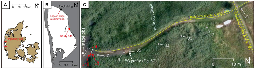
Figure 1. (A) Location of the lagoon Ringkøbing Fjord in Denmark and (B) location of field site along the coast of Ringkøbing Fjord. A station at Ringkøbing city provided bi-monthly lagoon stage and salinity observations between 1997 and 2015. (C) Overview of study site. Dots indicate piezometers in which discrete hand measurements of water levels were conducted (gray) or which were equipped with automated water level and salinity loggers (red; J8, J9, J10). Also shown is the location of the lagoon stage and salinity observation logger operating at the field site during July to December 2015.

In short, RKF is a shallow lagoon system with an average depth of 0.5 m (Kinnear et al., 2013). The lagoon is regulated by a sluice with the aim to keep the average water level at 0.25 m above sea level (masl) and the salinity between 6 and 15‰. Strong westerly winds ensure well-mixed salinity conditions in the lagoon water column. Vertical stratification can occur during wind speeds below 8 m/s when the sluice is opened to allow North Sea water to enter the lagoon (Kirkegaard et al., 2011). Skjern River contributes with an average of 50 m³/s freshwater. The surrounding of the lagoon is dominated by flat topography at elevations below 1 until 60 m from shore, where the terrain increases up to 3.5 masl (Figure 1C) followed by an again almost flat terrain. The regional geology is characterized by deep marine Paleogene clays at around 300 m depth, superimposed by an alternating sandy, silty, clayey Miocene formation (<10–20 m depth). The near surface geology at depth <20 m is composed of sandy Pleistocene glacio-fluvial sediments, which is locally intervened by silty units (Haider et al., 2015). The existence of buried paleo-channels composed of higher permeable sand modifies the deeper aquifers and can locally provide a hydraulic connection between lower and upper aquifers. The regional hydrogeological conditions around the Ringkøbing Fjord lagoon within the Pleistocene aquifer unit show an overall hydraulic head gradient perpendicular to shore, where hydraulic heads vary between 3 and 5 masl. Consequently, major groundwater contributions are expected to originate from east. A few observations from deeper wells indicate a vertical upward gradient and thus an exchange flux from deeper to shallower aquifers may take place locally (Kirkegaard et al., 2011). The field site containing 14 piezometers (J1–J14) was established by Müller et al. (2018) (Figure 1C) and only screen the upper shallow Pleistocene aquifer. Müller et al. (2018) showed that SGD varies seasonally and that a refreshing of the aquifer starts in October, where recharge is high leading to the observed regression of the saltwater wedge. The opposite occurs during summer, where recharge and consequently freshwater flows into the aquifer are reduced, leading to a saline wedge movement further onshore.

Data Collection

In the following data collection is presented, which serves, as input for the geological and hydrological model boundary.

Regional Borehole Data

Borehole data at seven locations (Supplementary Figure S1) was extracted from the Danish borehole database Jupiter (www.geus.dk).

ERT

The local near-surface geological structure was explored recording two electrical resistivity tomography (ERT) profiles with a Syscal Pro 96 switch unit (Iris Instruments) at the 30th September 2014. Profile A was measured perpendicular to the shoreline along a previous established piezometer transect (Figure 1C). Hereby a Wenner electrode configuration with 1 m spacing reaching a penetration depth of about 18 m was used. Profile B was recorded parallel to shore with a Wenner electrode configuration (5 m spacing) yielding a penetration depth of ~80 m (Figure 1C).The inversion software Res2dinv (Geometrics) was used to process the data.

Slug Test

Slug tests using the falling head method were conducted for each piezometer at the field site. Results were analyzed with the Hvorslev solution (Hvorslev, 1951). Three tests were conducted for most of the piezometers and mean values and their associated standard deviation (SD) are reported in the Supplementary Table S1.

Lagoon Stage and Salinity

Lagoon stage and salinity were measured from August 2014 until December 2015 using conductivity-temperature-depth (CTD) loggers (Diver®, Van Essen Instruments B.V., Delft, The Netherlands) (Figures 1B,C). Hydraulic head in all piezometer were measured on a seasonal basis between October 2014 and July 2015 (Müller et al., 2018). The piezometers J8, J9, and J10 were additionally equipped with CTD loggers to monitor hydraulic head and electrical conductivity (EC) in the period November 2014 until December 2015 (Figure 1C). The measured raw pressure heads were barometrically corrected, using measurements from a baro-Diver (Diver®, Van Essen Instruments B.V., Delft, The Netherlands) installed at the outside of the pipe at piezometer J11. EC values measured in μS/cm were recalculated to Total Dissolved Solids (TDS) using the empirical equation from Holzbecher (1998) (presented in Supplementary Material S 1.1).

Historical daily lagoon stage data were provided by the Danish coastal authority and were available from January 1997 until July 2015 from a station at Ringkøbing harbor north of the study site (from January 1999 stage was recorded every 15 min). Bi-monthly salinities were available from January 1997 until 2014 (Figure 2). Between 2014 and 2015 bi-monthly salinity measurements were provided by the Danish Nature Agency (Figure 3) also from north of Ringkøbing harbor (Figure 1B). Field site salinity data was available from 22nd July 2015 until 31st December 2015. Monthly summarized values are presented in Figure 2. Lagoon stages are relatively constant; however, minimum levels occurred between April and July, while high stages (approaching 0.2 m) occurred during November and February. The salinity variation was offset in time compared to the stage variation, with lowest salinities occurring from January to March and highest salinities occurring between June and October. This offset can be explained by high and low freshwater inputs from Skjern River in winter to spring time and summer to early fall, respectively. Lagoon water salinity varies from 7 to 15 g/L throughout the year (Figure 2).

FIGURE 2

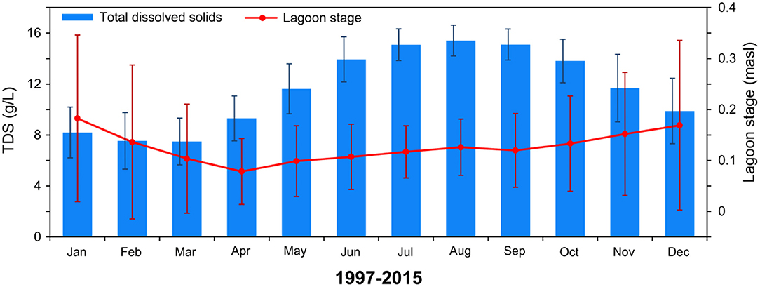
Figure 2. Monthly arithmetic mean and standard deviation (whiskers) of lagoon stage (line) relative to Danish Normal Null ref. elev. and salinity (columns) given as Total Dissolved Solids (TDS) of the Ringkøbing Fjord station (Figure 1B) between 1997 and 2015. Data provided by the Danish Nature Agency.

FIGURE 3

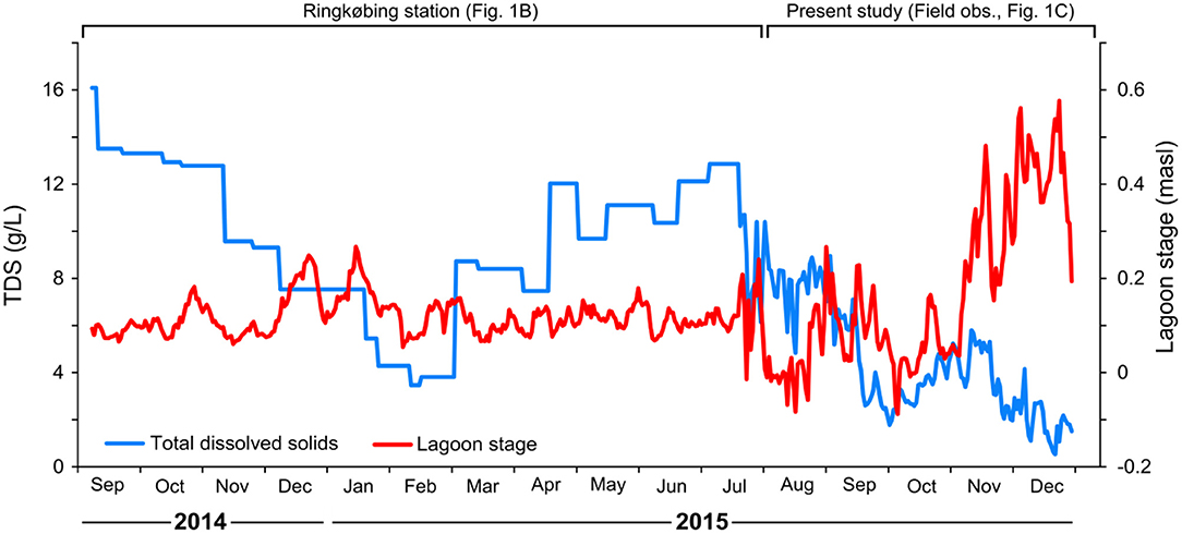
Figure 3. Lagoon stage (red line) and salinity (blue line; Total Dissolved Solids, TDS) between September 2014 and December 2015 compiled by data from the station at Ringkøbing city (Figure 1B) upsampled from bi-monthly to daily values, and from the logger operated at the field site (from 22 July 2015 forwards).

Numerical Model, Conceptualization, and Simulation Strategy

A 2D transient density-dependent groundwater flow and salt transport model was constructed to simulate groundwater and transport dynamics perpendicular to the shore along the ERT transect A using the FEM groundwater model Feflow (Diersch, 2014). The model domain extends 200 m in length with a varying thickness of 23–25 m. The top follows the topography and the bottom of the domain is kept horizontal. A triangulated mesh with 3,944 nodes and 7,368 elements is used, refined in the upper 2 m to better represent a capping peat layer present on site. To avoid numerical dispersion, Peclet numbers of 0.8 and 3 are defined for the finer and coarse grid parts, respectively (Figure 4).

FIGURE 4

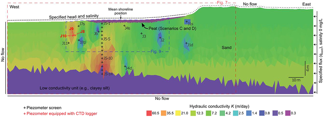
Figure 4. Model domain showing the boundary conditions and the interpolated spatial distribution of hydraulic conductivity K. q_east is represented by a sinusoidal water flux (sections Boundary Conditions, Fresh Groundwater Fluxes (q_east), Supplementary Table S2) with a solute concentration of 0 mg/L representing freshwater. Piezometer screen positions are indicated (crosses); the piezometers J8, J9 and J10 were equipped with conductivity-temperature-depth (CTD) loggers. Cropped extents of the model domain are shown in Figure 7 (indicated by red dashed line) and Figure 9 (blue dashed line).

The parametrization of hydrogeological parameters are based on the ERT and slug test results (sections Parameterization Based on Slug Test and Conceptual Hydrogeological Model). The major part of the aquifer is a heterogeneous sand layer sandwiched between a homogeneous capping peat layer with a thickness of 0.5 m, extending ~60 m perpendicular to the shore, and a homogeneous low permeable dipping layer at the bottom (section Conceptual Hydrogeological Model, Figure 6). The K distribution in the heterogeneous sand layer was interpolated via Kriging to the mesh using the slug test results (section Parameterization Based on Slug Test). The K of the surficial peat layer is set to 0.3 m/d based on literature values (Chason and Siegel, 1986). The low permeability unit at the bottom lacks direct measurements and therefore K is set to 0.5 m/d (the lowest measured at J1d and J7d). In a pre-calibration step where the warm-up period prior to the initialization period is used only, the anisotropy (K_v/K_h) was found by trial and error to a value of 0.1 for peat, sand, and the lower-K layer at the bottom (section Simulation Strategy and Scenarios).

Boundary Conditions

Semi-confined conditions are assumed at the top of the aquifer as a 0.5 m thick capping peat unit exists at the surface along the major part of the transect where most of the piezometers showed artesian conditions (Müller et al., 2018).

No flow conditions are specified at the bottom and the western boundary; in accordance with the low resistivities measured in the deeper part of the ERT profile (section Conceptual Hydrogeological Model). Transient boundary conditions are specified at the eastern boundary (q_east) where freshwater fluxes vary seasonally [section Fresh Groundwater Fluxes (q_east)]. The boundary conditions of the nodes influenced by stage fluctuation are switched between (transient) specified head (equal to lagoon stage) in case of flooding and otherwise specified flux (no flow). At this boundary a cross-boundary flux was derived, which serves as analog to seepage discharge. Onshore parts outside the tidal affected zone are defined as no flow boundary during the entire simulation period.

Simulation Strategy and Scenarios

The simulation strategy is outlined in Figure 5. To begin with, the model was run to a steady-state solution for hydraulic head, using non-variant lagoon stage and q_east boundary conditions and fresh groundwater across the whole model domain. To reach a more realistic initial head and salinity distribution under transient conditions, a “warm-up” period was applied. During the warm-up period, sinusoidal q_east, lagoon stage and salinity fluctuations (Figure 5), was set for 20 “average” years, based on long-term observations shown in Figure 2. Specifically, for the warm-up period, lagoon stage varied sinusoidal between 0.10 and −0.12 masl with an amplitude of 0.11, TDS varied sinusoidal between 3.1 and 15.2 g/L with an amplitude of 6.05 g/L, and q_east varied sinusoidal between 0.001 and 0.041 m/d with an amplitude of 0.02 m/d.

FIGURE 5

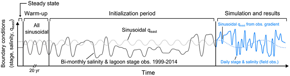
Figure 5. Illustration (not real data) of the transient boundaries of salinity and lagoon stage, indicated with just one line (gray) for simplicity, along with q_east applied during model runs. The model was run to stationarity. Then, a 20 year warm-up period with sinosoidal salinity, lagoon and q_east preceded a 15 year initialization period, which applied actual bi-monthly observations from the Ringkøbing station (Figure 1B). Lastly, the period September 2014–December 2015 used the compiled time series of Figure 3 along with a sinusoidal q_east determined by observed terrestrial-to-lagoon head gradient at the field site; results (model output) are shown for this period only. For each scenario, the model was run to stationarity and then continuously for the whole period of 36.5 years with transient boundary conditions.

The warm-up period was followed by a 16 year “initialization period” from 1999 to 2014, which consisted of observed bi-weekly (downscaled to daily) observed values of salinity and daily lagoon stage (Figure 3). Even though salinity measurements were already available from 1997, it was decided to discard data between 1997 and 1999 and start the implementation of observational data at the time when daily lagoon stage observation was available in 1999. The sinusoidal function for q_east as applied during the warm-up period was continued during the initialization periods.

In order to a find appropriate values for anisotropy (0.1), storage (0.1), longitudinal (0.5 m), and transverse dispersivity (0.05 m) a trial-and-error calibration of these parameters was conducted using boundary conditions of the combined warm-up and initialization periods (Figure 5). This calibration used R² as objective function in a comparison of simulated and hydraulic head observations (2014-2015).

Scenario A applies the above parameters and boundary conditions up to September 2014, and then applies the boundary conditions for lagoon stage and salinity between September 2014 and December 2015 (Figure 3). Scenario A in this way can be considered a “base case” relative to other Scenarios B–D, which tested sensitivity of q_east (Scenario B), presence of confining peat (Scenario C, Figure 4) and combined peat presence and dispersivity (Scenario D).

Scenarios B–D are described below and summarized in Table 1.

• Scenario B: Incoming freshwater flux q_east was adjusted to be within a range suggested by hydraulic head conditions at the field site [section Fresh Groundwater Fluxes (q_east), Supplementary Table S3]. A sinusoidal input function with a mean of 0.09 m/d and amplitude of 0.085 m/d is applied (Figure 5).

• Scenario C: A locally confining capping peat unit above sandy sediments was observed in the field and thus implemented to the domain (Figure 4) with a lower K of 0.5 m/d. Consequently, the base case storage coefficient for unconfined conditions became too high for semi-confined conditions, and therefore was lowered to 0.001.

• Scenario D: Effects of mixing dynamics (still in presence of confining peat) were investigated by increasing longitudinal and transverse dispersivity to 25 and 2.5 m, respectively.

TABLE 1

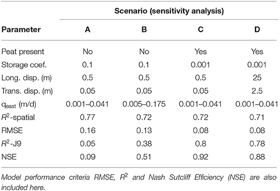
Table 1. Scenarios with respect to parameters to be calibrated against hydraulic head observation at piezometer J9 and input variables.

All scenarios were compared to daily-observed head and salinity data collected in piezometer J9 between November 2014 and July 2015. Piezometer J9 was chosen for simplicity because the neighboring piezometers J8 and J10 are placed within 1 m distance from J9. Thus, the model resolution is not sufficient to distinguish between these three piezometers. Model performance was evaluated using the coefficient of determination (R²) and Root Mean Square Error (RMSE) as well as the Nash-Sutcliffe Efficiency (NSE) to quantify temporal dynamic performance (Table 1). Average hydraulic heads from each scenario were additionally compared to average observed hydraulic heads at each piezometer location (R²-spatial). However, as the performance was similar and no extra temporal information can be gained, focus was given to the performance on transient data in the following.

Results

In the following the slug test results, ERT-measurements and incoming freshwater flux deviation are shown and interpreted in order to understand the implementation of hydrogeological boundary conditions in the model domain.

Parameterization Based on Slug Test

The average K on site (based on slug tests in the sand aquifer) is 17.54 m/d, with variations between 0.04 m/d at J6 and 67.8 at J5-12. For the majority of the piezometers, the standard deviation (SD) is low compared to the average hydraulic conductivity, while at J5-12 a high SD of 12.1 m/d is found (slug test results are listed in Supplementary Table S2). For J2, J6, and J11 only one replicate was obtained due to slow recovery. The overall range of K is typical for sand, while its slight decrease with depth may be indicative for the depositional environment where older sediments have been compacted over time at the lagoon shore. Two lenses with higher K-values (average 30.5 m/d) were found in the deeper parts at the shoreline and around the locations of J8-J10 and J5. Likewise, K-values <5 m/d were measured in onshore piezometers J1D, J2, J6, J4D-12. As K is not subject to calibration in the present study, average values based on three replicates were used as input for the kriging interpolation of the K-field in the model domain.

Fresh Groundwater Fluxes (q_east)

A range of fresh groundwater fluxes discharging into the transect area from east (q_east) were estimate based on (i) local hydraulic head gradient between the outermost piezometer of the piezometer transect J1d and the lagoon stage or ii) the regional hydraulic head gradients between inland wells (Supplementary Table S2) and the lagoon. Based on average hydraulic heads and average K-values of 17.5 m/d from the piezometer transect a Darcian flux range was delineated (Supplementary Table S2). Haider et al. (2015) defined the catchment boundary located at 5,500 m inland, eastwards from the field site. Only non-synchronous hydraulic head observations from regional wells within the catchment and with a screening depth in the upper aquifer (0–10 m below surface) were available. Therefore, an average hydraulic head among all regional wells was used. As their distance to the lagoon varies, a minimum and maximum distance was used to compute a gradient range. Darcian flux estimates based on local hydraulic head gradients (between the lagoon and well J1d) were between 0.004 and 0.15 m/d. Darcy fluxes based on regional boreholes yielded a lower range between 0.004 and 0.05 m/d (Supplementary Table S2). This approach is a crude approach to incorporate potential variations of the incoming fluxes from east. It reduces the aquifer between the lagoon until 5,500 m inland to a single K. This approach however, can add an uncertainty value to the local gradient observed, by incorporating regional hydraulic head trends.

Conceptual Hydrogeological Model

A fluvial-glacial sandy unit is found in the upper 10–15 m below surface (mbs) in the profiles of regional boreholes (Supplementary Figure S1B). Below, a clay unit with a thickness of ~7 m is observed. Another fluvial-glacial sand unit is mapped between 12 and 40 mbs as indicated by the three deepest boreholes. Finally, Miocene clay with incidents of sandy units are found in several boreholes at varying depths (Supplementary Figure S1B).

Resistivities <10 Ωm were measured 7 m offshore (western end) of profile A, down to a depth of 4 m (Figure 6A). This is followed by a plume-shaped zone with resistivities in the range 50–150 Ωm. The most off-shore part of the plume could be a result of intrusive lagoon water, while the remaining part could be a mixture of freshwater and saltwater. Higher resistivities above 250 Ωm were measured at depths between 2 and 7 m. Within the lower 10 m of the profile, resistivity decreased from 100 to 5 Ωm. Borehole data (Supplementary Figure S1), slug test results (Supplementary Table S1) and elevated resistivity consistently indicate sandy sediments between at 1 and 10 m depth. At depths larger than 10 m, low resistivity units appear in the ERT measurements, which may correspond to the clay units found in the Jupiter wells. According to the slug test results close to the shore (J5), the K-values were relatively high at depth >10 m, while at similar depth in J4, K was much lower. An enriched isotopic value of δ¹⁸O measured by Müller et al. (43) at this depth and relative high electrical conductivities (EC) at 10–13 m depth indicated saltwater intrusion, as isotopic enrichment and high EC were associated with intruding lagoon water (Müller et al., 2018). Therefore, it is argued that the low resistivities at depths >10 m were a result of saltwater and not low-permeable layers. In piezometers with screens deeper than 13 m depth, freshwater was found. Above 10 m, resistivity values in the range from 40 to 150 Ωm suggest sand saturated with lagoon water. Consequently, resistivity values of 30 Ωm beneath at depth below 10 m are attributed to clay containing freshwater (Figure 6A).

FIGURE 6

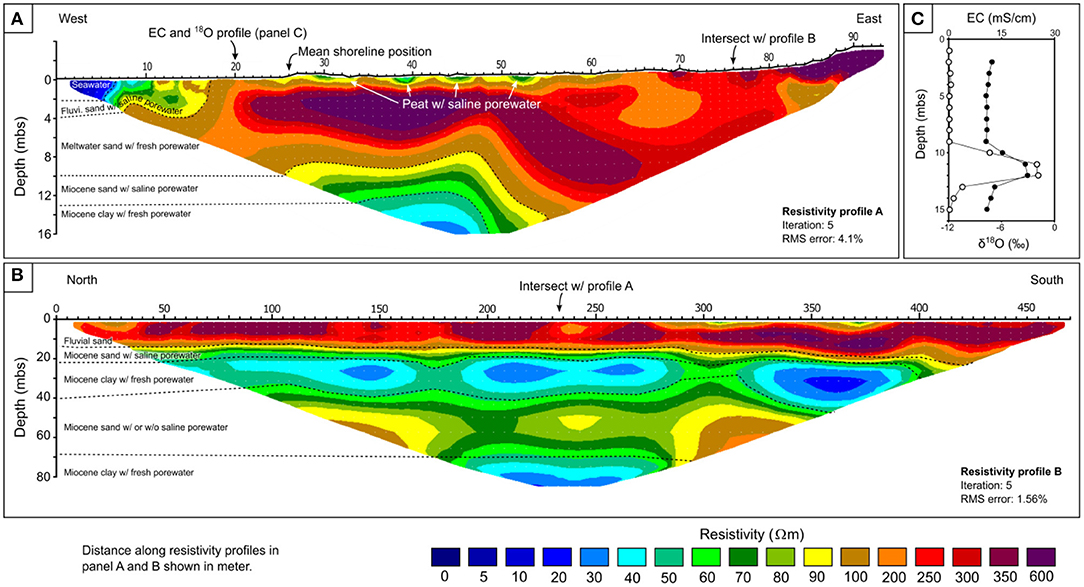
Figure 6. Electrical resistivity tomography profiles (A) perpendicular and (B) parallel to the shoreline (Figure 1C). (C) The δ¹⁸O and electrical conductivity (EC) profiles at piezometer J5 from Müller et al. (2018).

In the upper 0–2 m of the onshore part of profile A low resistivity values of 50–90 Ωm were measured reflecting peat material. Resistivity for peat depends on the conductance of peat pore water and the organic matrix. Resistivity within a peat layer typically increases with depth as mineral soil content increases (Comas et al., 2004). Values may be below 50 Ωm (Chambers et al., 2014), but lower ionic concentrations of peat pore water may result in resistivities >50 Ωm (Comas et al., 2004). Therefore, the low resistivity values in this upper layer are likely caused by the presence of peat. However, increased ionic concentration caused by temporarily propagation of the lagoon stage may also lead to lower resistivity.

Resistivity profile B (Figure 6B) reached a depth of 80 m and its interpretation was based on findings from profile A. In the upper 10–15 m an undulating structure with values above 150 Ωm appeared, representing fresh meltwater sand. At depths of 15–22 m a transition zone with values between 50 and 150 Ωm were recorded, which could correspond to the Miocene sand unit containing intruded saltwater. Below, a zone of resistivities <40 Ωm to a depth of ~40 m were observed. Although airborne geophysical data from the area indicated a clear salt-water wedge across all layers (Kirkegaard et al., 2011), this zone is believed to contain Miocene clay containing freshwater because regional borehole data (Supplementary Figure S1) indicate clay units at those depths. Between 40 and 60 m depths, the resistivity increased again to 50–150 Ωm. This coincides with Miocene sand observations in the regional boreholes (Supplementary Figure S1). Yet, from the ERT profile A, as well as from airborne geophysical data (Kirkegaard et al., 2011), saltwater may be present in these resistivity ranges and depths. The low resistivity at the bottom of the profile represents a Miocene clay freshwater unit, an interpretation that is supported by airborne geophysics (Kirkegaard et al., 2011). Depth information of the lowest Miocene freshwater unit in both ERT profiles A and B, indicate that clay unit to dip from west to east.

Model Results and Sensitivity Analysis

Figure 7 shows the simulation results of the scenario runs A–D investigating the effect of different parameters.

FIGURE 7

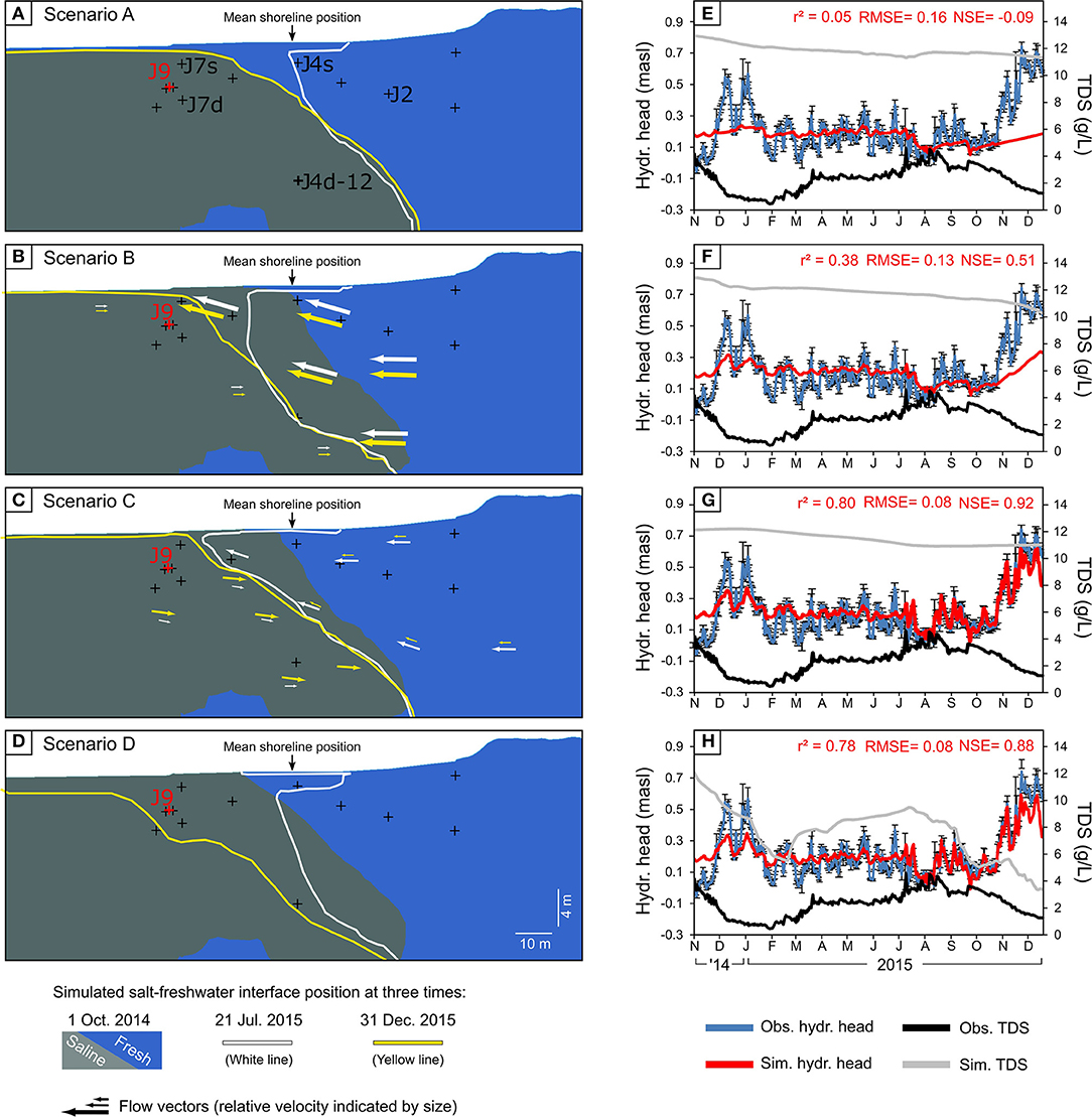
Figure 7. Simulation results of Scenarios A–D. (A–D) Temporal movement of the salt-freshwater interface, defined at TDS 5 g/L, in October 2014 (gray-blue shading), July 2015 (white line), and October 2015 (yellow). Selected flow vectors indicate direction and relative flow magnitudes in July 2015 (white arrows) and December 2015 (yellow). See Figure 4 for shown extent of model domain. (E–H) Simulated and observed hydraulic head and TDS at piezometer screen J9, including summary statistics. Whiskers indicated daily standard deviation calculated from hourly recorded head values.

Seasonal Variation of Saltwater Intrusion (Scenario A)

Scenario A is used to test the overall performance of the model conceptualization. The Scenario A model did not contain a peat unit on top of the sand, and it used the dynamic lagoon and groundwater flow boundary conditions (Table 1). This scenario did not reproduce the temporal dynamics of hydraulic head or salinity concentration changes in piezometer J9 (R² = 0.05, RMSE = 0.16 m, and NSE = −0.09, Figure 7E; Table 1). The dynamics of simulated hydraulic heads were damped compared to the observed heads. The high hydraulic heads in the beginning and the increasing hydraulic heads at the end of the simulation period were not reproduced by the model. Furthermore, simulated salinities were too high and exhibit too little seasonal dynamics, e.g., the observed decrease in salinity in winter and increasing salinity in summer was not reproduced by the model. The saltwater wedge movement, caused by the dynamic changes in the lagoon stage and salinity, was limited to the upper third of the aquifer (Figure 7A). The decreasing inflow from east during the summer periods caused the wedge to move ~20 m toward shore in the upper 7 m of the aquifer. To test the sensitivity and improve model performance, the model parameters and boundary conditions were adjusted in the remaining scenarios.

Effect of Freshwater Inflow (Scenario B)

The only change from Scenario A to B was the magnitude of the dynamic freshwater groundwater boundary, where the input flux q_east was allowed to vary between 0.005 and 0.175 m/d (Table 1). This represents an increase by a factor of 4–5 compared to the Scenario A. Increasing groundwater inflow improved the hydraulic head simulation compared to Scenario A, as R² increased to 0.3, while the RMSE only decreases slightly to 0.13 m. An improvement in simulating hydraulic head dynamics is reflected in an increase in NSE to 0.50. Nevertheless, simulated salinities were still much higher than those observed with an overall decreasing tendency (Figure 7F). Between October 2014 and July 2015 the simulated saltwater wedge retreated by 12 m across the whole thickness of the aquifer. While in the upper part of the aquifer, the wedge continues to retreat by another 16 m until December 2015 (Figure 7B).

Effect of Peat Layer and Lower Storage (Scenario C)

The q_east flux was reset to the values from Scenario A. A peat unit was added to the top and the storage parameter of the sand unit was reduced by a factor of 100 (to 0.001), now better reflecting a confined system. More hydraulic head dynamics now appeared in the simulation results (Figure 7G), which is especially visible from the period starting in July 2015, where lagoon observations were made directly at the field site. This improves the simulation markedly, which is best expressed by the very high NSE of 0.94, as well as the low RMSE of 0.08 m. Nevertheless, simulated salinities were still too high and did not follow the observed dynamics. Freshwater inflow displaced the saltwater wedge in the upper 5 m by ~25 m offshore between October 2014 and July 2015. The toe of the wedge remained at the same location as in October (Figure 7C). Müller et al. (2018) observed a freshwater lens thickness at J4 of at least 12 m in February 2015, while a thickness of ~6 m was simulated.

Dispersion Effects (Scenario D)

For Scenario D, the peat unit and the low storage parameter of the confined layers were maintained while dispersivities were increased (α_L = 25 m, α_T = 2.5 m). Model performance did not improve further as R² decreased slightly, while RMSE and NSE remained high (Figure 7H). However, the character of the saltwater wedge movement changed distinctively (Figure 7D). Between October and July the saltwater-freshwater interface in the upper very shallow part (upper 1.5 m) transgressed further into the aquifer, while at larger depth the wedge regressed toward shore with a constant toe location. Between July 2015 and December 2015 the boundary flux q_eas increased, causing the interface to move ~40 m in offshore direction. This formed a shallow freshwater lens in the upper part of the aquifer beneath the lagoon bed. Increasing dispersion parameters takes into account geological heterogeneity not represented at the presented model scale, which is expressed in an increase of the saltwater affected areas within the model domain. Therefore, simulated salinities decreased, yielding differences of 2 g/L toward the end of the simulation period between the simulation and the observation at J9 (Figure 7H).

Discussion

Scenario Results

By facilitating measured stage and salinity values and a dynamic freshwater inflow component based on well observations, the model was able to produce density dependent flow and salinity dynamics of the near coastal aquifer at Ringkøbing Fjord, where a dynamic saltwater wedge in the shallow parts of the aquifer is present.

For the current model study, with the aim to reproduce observed saltwater wedge dynamics and to indicate the spatial and temporal extent of the saltwater wedge dynamics at Ringkøbing fjord.

Evaluation criteria for model performance during different scenario runs (parameter testing) were primarily based on quantitative performance criteria (RMSE, R², NSE), while qualitative performance was secondary. In the following discussion, the approximate extension of the saltwater wedge can be seen at a threshold value of 5 g/L (Figures 8, 9). Because lagoon salinity never reaches values below 5 g/L, this threshold is a good indicator for the presence of a strong fraction of seawater. Values below 5 g/L indicate a mixture between fresh and saline water.

FIGURE 8

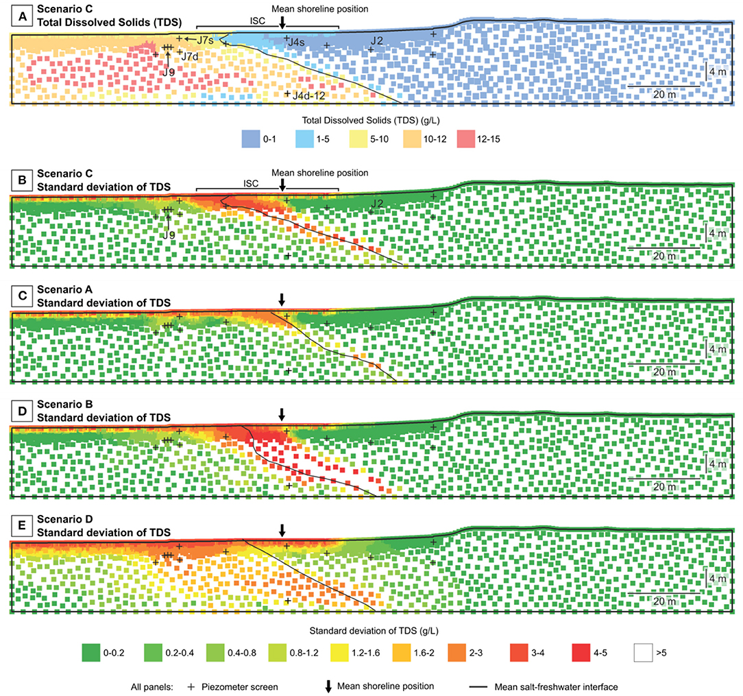
Figure 8. (A) Spatial distribution of average TDS as simulated in Scenario C. (B–E) Standard deviations over the whole simulation period for Scenarios A–D, respectively. In all panels, the black line indicates the average position of the salt-freshwater interface, defined at TDS 5 g/L. This figure shows the entire model domain of Figure 4, yet in a near-true vertical to horizontal scale (see scale bars).

FIGURE 9

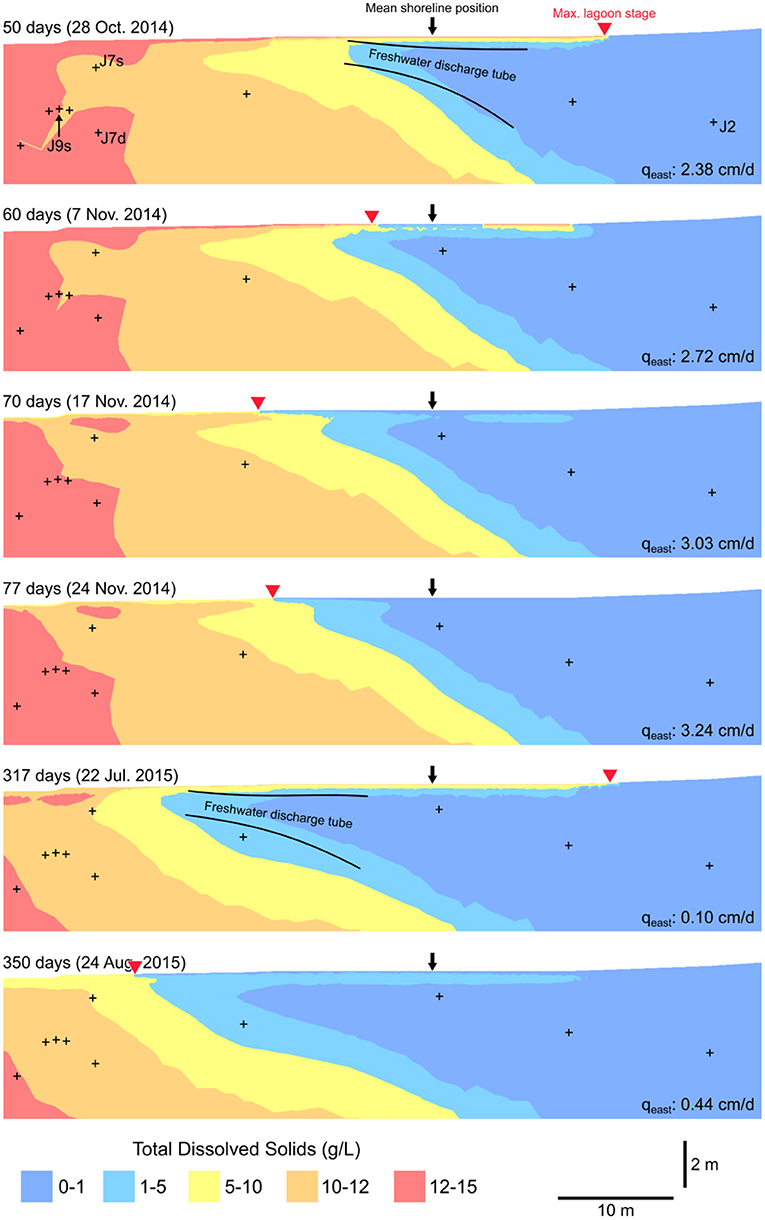
Figure 9. Simulated transient behavior of the salt-freshwater interface during a wet period (autumn) and dry period (summer) for Scenario C. The value of q_east results from the sinusoidal input function at each particular time step. A temporal freshwater (TDS < 5 g/L) discharge tube forms below the lagoon bed in response to low recharge periods (small q_east in summer periods), and diminishes during winter recharge periods in response to increased q_east.

Inland water table fluctuations are closely related to recharge dynamics in the catchment, which in reverse may modify the saltwater wedge dynamics (Kohout, 1960; Michael et al., 2005). For Ringkøbing Fjord, responses of inland water tables were expressed as changing freshwater inflows through the eastern model boundary, which generally resulted in a regression/-transgression of the saltwater wedge. However, changing the relative magnitude of the incoming freshwater improved objective model performance, while the biggest improvement of the model was achieved by adding a capping peat layer to the top of the domain (Table 1). This suggest minor importance of inland recharge dynamics compared to local geological structures. Even though, increased spatial saltwater wedge dynamics are suggested based on SD values when inland fluxes are increased, compared to the effect of local geological features (Figures 8B,D, respectively), this conclusion is biased. The higher simulated inland water fluxes in Scenario B, is rather caused by a constantly offshore displacement of the interface, that eventually forms a new equilibrated situation. Such wedge movement to a new equilibrated position further offshore is in line with the study by Müller et al. (2018) and Duque et al. (2019). In both studies, the shallow wedge is found between piezometer J6 and J7. This suggests that increasing fluxes four to five times based on local and regional derived well measurements [section Fresh Groundwater Fluxes (q_east)] is necessary to reflect a realistic saltwater wedge position, despite the missing wedge dynamics.

Nevertheless, for the best performing Scenario C the average location of the saltwater wedge may not be in line with the observations from Müller et al. (2018) nor by Duque et al. (2019). Yet the simulated saltwater wedge location in August 2015 (Figure 9, bottom panel) coincides rather well with observations made in those earlier studies during summer month. The present model simulates a narrow zone of salinities between 1 and 5 g/L at the top part of the onshore area (Figure 8). This may be appointed to an ISC (Robinson et al., 2006), due to the propagation of saline lagoon water to onshore areas induced by stage changes. The ISC in Scenario C can extend up to 30 m onshore from the shoreline. Yet, resulting density driven subsurface dynamics are limited to the shallow aquifer (Figure 8B), where high SDs are found. This affects mostly the area between J7S, J7D, and J4D-12 with variations up to 5 g/L while the area around J9 is rather unaffected by the seasonal wedge dynamic expressed in SD values around 0.4–0.8 g/L.

Reasons for the stagnant saltwater wedge at greater depth are suggested to be due to density dynamic flows counteracting freshwater flows. During times of lower freshwater inflow (July- white arrows in Figure 7C) show a larger magnitude than flow vectors pointing from lagoon to land. Yet, during periods of high recharge, the relative size of the vectors is reversed and a density induced counter flux from sea to shore is present. This may be counterintuitive, but points toward the influence of infiltrating seawater from previous summer periods having higher salinities (Figure 2), which first shows its effect in the subsurface during the consecutive autumn period, where it counteracts high freshwater flows.

The simulated salinities at the piezometer J9 are always higher than the observed. Reasons for this may be small scale density driven flows beneath the lagoon bed, which cause a more complex and dynamic salinity distribution (Duque et al., 2019), a result of e.g., fingering (Van Dam et al., 2014). Adopting the approach by Wooding et al. (1997) for current conditions at Ringkøbing Fjord [evaporation ~ 157 mm/year, maximum density difference Δρ = 0.21, detailed equations summarized in Supplementary Material S 1.3, macroscopic Rayleigh number and Boundary Rayleigh number of 7.3^*10⁵ and 8.7^*10³, respectively are derived. This leads to instable boundary conditions where fingering occur. This dynamic condition can be captured by the present model (Figure 9), but is hardly captured by a single well observation and would probably require additional piezometers, screening across the saltwater-freshwater interface.

To reduce salinities at J9, an alternative model setup was tested by increasing dispersion (Scenario D) to account for geological heterogeneity and hence more mixing in the absence of temporal dynamics in flow (Goode and Konikow, 1990). Salinities were reduced at J9, likely a consequence of a more dynamic saltwater wedge. Simulated transgression/regression dynamics were furthermore more significant between October 2014 and July 2015 (Figure 7D), reflected by the elevated SD in Scenario D (Figure 8E). However, high dispersivities do not explain the actual underlying mechanisms forming a wider wedge, but are often used to compensate the under-representation of wedge dynamics due to geological heterogeneities (Werner et al., 2013). Consequently, from Scenarios C to D it can be concluded, that at small scale, geological heterogeneity has a strong impact on the dynamic wedge distribution and may not be captured satisfactorily using an interpolated K distribution with high dispersivities.

Additional factors affecting the temporal and spatial salinity dynamics may be caused by the simplified 2D-setup of the model domain. Micro-bays or complex macro geological structures, e.g. buried valleys, existing at Ringkøbing Fjord (Kirkegaard et al., 2011; Kinnear et al., 2013) cause flow paths to have an odd angle to the shore and may alter transport dynamics significantly as shown by Meyer et al. (2018, 2019) for an area 100 km further south. Hence, a 3D simulation may be more appropriate when representing wedge dynamics (Werner et al., 2013) at Ringkøbing Fjord. Other studies (Li and Jiao, 2003) have shown a close relation between upper and lower aquifer systems in coastal areas via leakage. Additional freshwater input from a leaky lower aquifer cannot be ruled out, and would reduce the salinity concentrations in the upper aquifer.

Temporal Subsurface Density Dynamics

Scenario C describes the dynamics of the hydraulic heads best (Figure 7G) and the development of an ISC based on those scenario results is discussed above.

The subsurface density dynamics are shown in Figure 9 throughout the course of a full hydrological year (October–September). In October and July, high lagoon stages cause a flooding of the flat near shore area up to 30 m onshore, delivering and depositing high saline waters from the lagoon water onto fresh peat soils creating an intertidal salinity cell (ISC). Consequently, an inverse density pattern forms a freshwater discharge tube (Michael et al., 2005; Vandenbohede and Lebbe, 2006; Robinson et al., 2007; Heiss and Michael, 2014) where saline waters overly freshwater. This prevents groundwater from discharging into the adjacent peat covered wetland and forces the fresh groundwater to discharge around the average shoreline (see Figure 8B, values <1 g/L below peat area of >5 g/L). Based on the simulation the ISC at RKF is suggested to be maintained for 1–2 months (between July and August, Figure 9 in response to lower freshwater inflows from east (October–November 2014), but also due to stage changes (July and August 2015). This stands in contrast to other systems, where the persistence (growing and waning) of the ISC may range from 4 weeks (Abarca et al., 2013) to only 14 days (Robinson et al., 2007) strongly depending on the magnitude of the tide and the beach morphology. Continuous increase of the incoming fresh groundwater (q_east) causes a progressive dilution of the ISC, refreshing the peat as well as moving the saltwater-freshwater interface further offshore. Due to the existence of the ISC nutrient rich fresh groundwater moves its discharging area from peat/organic rich soils to the more sand containing sediment-water interface. Nevertheless, the model results suggests that the deeper parts of the near coastal aquifer are less influenced by groundwater, where the saltwater toe location remains relatively constant (Figure 9, yellow areas). Consequently, this simulation modifies the hypothesis from Müller et al. (2018), where a dynamic wedge over the full depth of the shallow aquifer is proposed. Because the summer simulation of the saltwater wedge coincides well with Müller et al. (2018) and Duque et al. (2019) summer observation, it must be concluded that most saltwater wedge dynamics appear in the shallow part of the aquifer above 6 m.

The biogeochemical dynamics of the saltwater-freshwater interface are governed by oxic-anoxic processes, altering nutrient mobilization and pathways (Moore and Joye, 2021). Hence, a temporal and spatial dynamic saltwater wedge has the potential to modify nutrient dynamics. Nutrient dynamics are further impacted by groundwater residence times as certain nutrient reactions appear on short timescales (e.g., NH₄ release, Steinmuller and Chambers, 2018) and are seasonally dependent (N-mineralization peak in autumn, Tamborski et al., 2015). Thus, the timing of nutrient export pulses to the lagoon may be further complicated by saltwater wedge dynamics.

Simulated cross-boundary fluxes (SGD analog) across the top land-surface boundary are in the same order of magnitude as observed seasonal and spatial fluctuations of SGD (published in Müller et al., 2018). Simulated SGD on 1st October 2014 is 2.9 while 3.7 cm/d was observed with seepage meters. Simulated SGD on 21st July 2015 averages to 2.5 cm/d, which is a factor 1.5 times higher than observed fluxes of 1.6 cm/d that day. SGD variation is not a unique function of recharge dynamics (q_east), as during 1st October 2014 q_east is 0.09 m/d as opposed to 0.01 m/d at 21st July 2015. Eventhough the simulated seasonal difference is less significant than for the observation, the peak SGD rates are well-matched and the spatial pattern of SGD is well-reproduced. SGD rates at Ringkøbing Fjord are among the average values of SGD rates observed in different lagoon and coastal environments across the earth (Taniguchi et al., 2002; McCoy and Corbett, 2009). Seasonal fluctuations of SGD and associated fresh or saline components can have direct environmental impact (Zhang et al., 2020) as they modify subsurface and surface water biogeochemical settings (Santos et al., 2021) and microbial communities (Ruiz-González et al., 2021). For the Ringkøbing Fjord lagoon and near surface aquifer system the magnitude of SGD is also expected to have large impacts. Estimated salinity concentrations (Supplementary Material S 1.4) of the seepage flux from October 2014 measurements of Müller et al. (2018) show that with distance from shore the lagoon water contribution increases (Figure 10) from roughly 25 to 75%. Henceforth, despite a general upward flow direction, an intruded saline lagoon water component is mixed with upwelling groundwater and discharged as SGD into the lagoon. This documents the existing complex circulations patterns beneath the lagoon as well as the potential impact for nutrient cycling in the near surface aquifer as well as the lagoon.

FIGURE 10

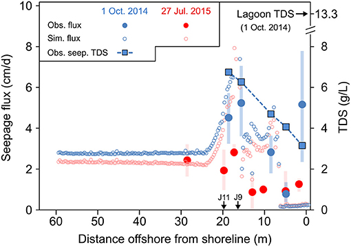
Figure 10. Left y-axis: Observed (filled dots; Müller et al., 2018) and simulated (open dots; Scenario C, this study) seepage flux on 1 October 2014 (blue) and 27 July 2015 (red) vs. distance offshore from shoreline. Shaded whiskers indicate standard deviations (color coded). Right y-axis: Observed TDS of seepage water (blue squares) and lagoon water (arrow) as measured on 1 October 2014. Location of J9 and J11 indicated on x-axis for reference.

This study therefore strongly suggests taking into account such saltwater wedge seasonality, when the biogeochemistry of near coastal areas is studied.

Conclusion

In order to understand nutrient cycling in near-coastal aquifers, groundwater flow and density dynamics need to be well-understood. This study shows variable subsurface circulation and salinity patterns in response to varying freshwater inputs and stage change induced flooding. Most prominent variations of salinity patterns occur in the shallow subsurface where an ISC is formed during flooding, while an offshore movement of the saltwater wedge occurs in response to elevated freshwater inputs during high recharge periods.

In this study the subsurface geology was explored by combining regional borehole data, ERT-measurements and slug test derived hydraulic conductivities. This was used to construct a model simulating transient flow and density dynamics in order to assess the seasonal dynamics at a saltwater-freshwater interface. An essential feature of the model was the application of dynamic boundary conditions at the lagoon bed and incoming freshwater fluxes. Thereby the stage dynamics of the system are represented with higher accuracy compared to other groundwater density driven model codes. Head observations were simulated with great accuracy, while absolute salinity concentrations are not produced with accuracy, but salinity dynamics are well-represented. Among other parameters tested for sensitivity, dispersion parameters improved the salinity concentrations substantially. It is discussed that the geological heterogeneity derived from local field site observations through Kriging still underrepresents the actual aquifer heterogeneity and the 2D representation of the model domain may not be sufficient. Earlier field investigations suggested a strong response of the saltwater wedge to changes in freshwater fluxes across the whole shallow aquifer depth. This model challenges this hypothesis and suggests that such dynamics are more likely to occur in the shallowest part of the aquifer at Ringkøbing Fjord.

The formation of an ISC, which persists for ~2 months throughout the summer and diminishes after 1 month during wetter periods will affect the timing and spatial extent of nutrient delivery into the adjacent lagoon and nutrient dynamics within the near shore aquifer. Nutrient delivery to lagoons occurs directly through SGD rates. From earlier studies SGD is shown to vary seasonally, while the simulation of the present study captures the magnitude and spatial pattern of SGD well. SGD is shown to be composed of a mixture of freshwater and recirculated lagoon water, where the latter increases with distance from shore. Hence, the diverse temporal and spatial SGD pattern is a potential strong driver in modifying the biogeochemistry lagoons and their adjacent aquifers.

Data Availability Statement

The raw data supporting the conclusions of this article will be made available by the authors, without undue reservation.

Ethics Statement

Written informed consent was obtained from the individual(s) for the publication of any potentially identifiable images or data included in this article.

Author Contributions

SM, PE, SJ, TS, and RM: conceptualization and design. SM and RM: methodology. SM: software modeling and writing-original draft preparation. SM, RM, SJ, and TS: writing-review and editing, contributed to manuscript revision, read, and approved the submitted version. PE: supervision and reviewed the first draft of the manuscript. All authors contributed to the article and approved the submitted version.

Funding

This work was supported by the Center for Hydrology (HOBE—www.hobe.dk), funded by the Villum foundation. DHI provided a free 1-year academic license for Feflow.

Conflict of Interest

The authors declare that the research was conducted in the absence of any commercial or financial relationships that could be construed as a potential conflict of interest.

Publisher's Note

All claims expressed in this article are solely those of the authors and do not necessarily represent those of their affiliated organizations, or those of the publisher, the editors and the reviewers. Any product that may be evaluated in this article, or claim that may be made by its manufacturer, is not guaranteed or endorsed by the publisher.

Acknowledgments

Sadly, our collaborator and supervisor PE passed away before the submission of the final version of the manuscript. Jola Kazmierczak, Evi Sebok, Bethany Nielsen, and Carlos Duque are thanked for their commitment during field work. SM accepts responsibility for the integrity and validity of the data collected, analyzed and simulated.

Supplementary Material

The Supplementary Material for this article can be found online at: https://www.frontiersin.org/articles/10.3389/frwa.2021.773859/full#supplementary-material

References

Abarca, E. (2006). Seawater Intrusion in complex geological environments (PhD thesis). Universitat Politecnica de Catalunya, Barcelona, Spain.

Google Scholar

Abarca, E., Karam, H., Hemond, H. F., and Harvey, C. F. (2013). Transient groundwater dynamics in a coastal aquifer: the effects of tides, the lunar cycle, and the beach profile. Water Resour Res. 49, 2473–2488. doi: 10.1002/wrcr.20075

PubMed Abstract | CrossRef Full Text | Google Scholar

Baldwin, D. S., Rees, G. N., Mitchell, A. M., Watson, G., and Williams, J. (2006). The short-term effects of salinization on anaerobic nutrient cycling and microbial community structure in sediment from a freshwater wetland. Wetlands. 26, 455–464. doi: 10.1672/0277-5212(2006)26[455:TSEOSO]2.0.CO;2

CrossRef Full Text | Google Scholar

Barnes, R. S. K. (1980). Coastal Lagoons- The Natural History of a Neglected Habitat, 1st Edn. Cambridge: Cambridge University Press, 120.

Google Scholar

Burnett, W. C., Aggarwal, P. K., Aureli, A., Bokuniewicz, H., Cable, J. E., Charette, M. A., et al. (2006). Quantifying submarine groundwater discharge in the coastal zone via multiple methods. Sci. Total Environ. 367, 498–543. doi: 10.1016/j.scitotenv.2006.05.009

PubMed Abstract | CrossRef Full Text | Google Scholar

Chambers, J. E., Wilkinson, P. B., Uhlemann, S., Sorensen, J. P. R., Roberts, C., Newell, A. J., et al. (2014). Derivation of lowland riparian wetland deposit architecture using geophysical image analysis and interface detection. Water Resour. Res. 50, 5886–5905. doi: 10.1002/2014WR015643

PubMed Abstract | CrossRef Full Text | Google Scholar

Charette, M. A., and Sholkovitz, E. R. (2002). Oxidative precipitation of groundwater-derived ferrous iron in the subterranean estuary of a coastal bay. Geophys Res Lett. 29, 85-1–85-4. doi: 10.1029/2001GL014512

CrossRef Full Text | Google Scholar

Chason, D. B., and Siegel, D. I. (1986). Hydraulic conductivity and related physical properties of peat, lost river peatland, northern Minnesota. Soil Sci. (USA). 142, 91–99. doi: 10.1097/00010694-198608000-00005

CrossRef Full Text | Google Scholar

Coluccio, K. M., Santos, I. R., Jeffrey, L. C., and Morgan, L. K. (2021). Groundwater discharge rates and uncertainties in a coastal lagoon using a radon mass balance. J. Hydrol. 598:126436. doi: 10.1016/j.jhydrol.2021.126436

CrossRef Full Text | Google Scholar

Comas, X., Slater, L., and Reeve, A. (2004). Geophysical evidence for peat basin morphology and stratigraphic controls on vegetation observed in a Northern Peatland. J. Hydrol. 295, 173–184. doi: 10.1016/j.jhydrol.2004.03.008

CrossRef Full Text | Google Scholar

Cooper, H. H. (1959). A hypothesis concerning the dynamic balance of fresh water and salt water in a coastal aquifer. J. Geophys. Res. 64, 461–467. doi: 10.1029/JZ064i004p00461

CrossRef Full Text | Google Scholar

Corbett, D. R., Chanton, J., Burnett, W., Dillon, K., Rutkowski, C., and Fourqurean, J. W. (1999). Patterns of groundwater discharge into Florida Bay. Limnol. Oceanogr. 44, 1045–1055. doi: 10.4319/lo.1999.44.4.1045

CrossRef Full Text | Google Scholar

Diersch, H.-J. G. (2014). “Discrete feature modeling of flow, mass and heat transport processes.” in: FEFLOW: Finite Element Modeling of Flow, Mass and Heat Transport in Porous and Fractured Media, eds. H.-J. G. Diersch (Berlin, Heidelberg: Springer), 711–56.

Google Scholar

Duque, C., Haider, K., Sebok, E., Sonnenborg, T. O., and Engesgaard, P. (2018). A conceptual model for groundwater discharge to a coastal brackish lagoon based on seepage measurements (Ringkøbing Fjord, Denmark). Hydrol. Process.. 32, 3352–3364. doi: 10.1002/hyp.13264

PubMed Abstract | CrossRef Full Text | Google Scholar

Duque, C., Jessen, S., Tirado-Conde, J., Karan, S., and Engesgaard, P. (2019). Application of stable isotopes of water to study coupled submarine groundwater discharge and nutrient delivery. Water. 11:1842. doi: 10.3390/w11091842

CrossRef Full Text | Google Scholar

Gibbes, B., Robinson, C., Li, L., and Lockington, D. (2007). Measurement of hydrodynamics and pore water chemistry in intertidal groundwater systems. J. Coast. Res. 50:12. Available online at: http://www.jstor.org/stable/26481708

Google Scholar

Goode, D. J., and Konikow, L. F. (1990). Apparent dispersion in transient groundwater flow. Water Resour. Res. 26, 2339–2351. doi: 10.1029/WR026i010p02339

CrossRef Full Text | Google Scholar

Haider, K., Engesgaard, P., Sonnenborg, T. O., and Kirkegaard, C. (2015). Numerical modeling of salinity distribution and submarine groundwater discharge to a coastal lagoon in Denmark based on airborne electromagnetic data. Hydrogeol. J. 23, 217–233. doi: 10.1007/s10040-014-1195-0

CrossRef Full Text | Google Scholar

Haines, P. E. (2006). Physical and chemical behavior and management of Intermittently Closed and Open Lakes and Lagoons (ICOLLs) in NSW (PhD.). Brisbane, QLD: Griffith Centre for Coastal Management, School of Environmental and Applied Sciences, Griffith University.

Google Scholar

Heiss, J. W., and Michael, H. A. (2014). Saltwater-freshwater mixing dynamics in a sandy beach aquifer over tidal, spring-neap, and seasonal cycles. Water Resour. Res. 50, 6747–6766. doi: 10.1002/2014WR015574

PubMed Abstract | CrossRef Full Text | Google Scholar

Holzbecher, E. O. (1998). Modeling Density-Driven Flow in Porous Media: Principles, Numerics Software. Berlin Heidelberg: Springer-Verlag. Available online at: https://www.springer.com/gp/book/9783540636779 (accessed September 6, 2021).

Google Scholar

Hopkinson, C. S., and Giblin, A. E. (2008). “Nitrogen dynamics of coastal salt marshes,” in: Nitrogen in the Marine Environment. (Elsevier), 991–1036. Available online at: https://linkinghub.elsevier.com/retrieve/pii/B9780123725226000220 (accessed September 6, 2021).

Google Scholar

Hvorslev, J. (1951). Time Lag and Soil Permeability in Ground-Water Observations. (Vicksburg, Mississippi: U.S.Army), 57. (Corps of Engineers). Report No.: 36. Available online at: http://luk.staff.ugm.ac.id/jurnal/freepdf/Hvorslev1951-USACEBulletin36.pdf (accessed November 16, 2021).

Google Scholar

Ji, T., Du, J., Moore, W. S., Zhang, G., Su, N., and Zhang, J. (2013). Nutrient inputs to a Lagoon through submarine groundwater discharge: the case of Laoye Lagoon, Hainan, China. J Marine Syst. 111–112, 253–262. doi: 10.1016/j.jmarsys.2012.11.007

CrossRef Full Text | Google Scholar

Joyce, C. B., Vina-Herbon, C., and Metcalfe, D. J. (2005). Biotic variation in coastal water bodies in Sussex, England: Implications for saline lagoons. Estuarine Coastal Shelf Sci. 65, 633–644. doi: 10.1016/j.ecss.2005.07.006

CrossRef Full Text | Google Scholar

Jun, M., Altor, A. E., and Craft, C. B. (2013). Effects of increased salinity and inundation on inorganic nitrogen exchange and phosphorus sorption by tidal freshwater floodplain forest soils, Georgia (USA). Estuaries Coasts. 36, 508–518. doi: 10.1007/s12237-012-9499-6

CrossRef Full Text | Google Scholar

Kinnear, J. A., Binley, A., Duque, C., and Engesgaard, P. K. (2013). Using geophysics to map areas of potential groundwater discharge into Ringkøbing Fjord, Denmark. Lead. Edge. 32, 792–796. doi: 10.1190/tle32070792.1

CrossRef Full Text | Google Scholar

Kirkegaard, C., Sonnenborg, T. O., Auken, E., and Jørgensen, F. (2011). Salinity distribution in heterogeneous coastal aquifers mapped by airborne electromagnetics. Vadose Zone J. 10, 125–135. doi: 10.2136/vzj2010.0038

CrossRef Full Text | Google Scholar

Kjerfve, B. (1994). “Chapter 1 coastal lagoons,” in: Elsevier Oceanography Series, eds. B. Kjerfve. (Elsevier), 1–8. (Coastal Lagoon Processes; vol. 60). Available online at: https://www.sciencedirect.com/science/article/pii/S0422989408700060 (accessed September 8, 2021).

Google Scholar

Kohout, F. A. (1960). Cyclic flow of salt water in the Biscayne aquifer of southeastern Florida. J. Geophys. Res. 65, 2133–2141. doi: 10.1029/JZ065i007p02133

CrossRef Full Text | Google Scholar

Li, H., and Jiao, J. J. (2003). Tide-induced seawater–groundwater circulation in a multi-layered coastal leaky aquifer system. J. Hydrol. 274, 211–224. doi: 10.1016/S002-1694(02)00413-4

CrossRef Full Text | Google Scholar

Li, L., Barry, D. A., Stagnitti, F., and Parlange, J.-Y. (1999). Submarine groundwater discharge and associated chemical input to a coastal sea. Water Resour. Res. 35, 3253–3259. doi: 10.1029/1999WR900189

PubMed Abstract | CrossRef Full Text | Google Scholar

McCoy, C. A., and Corbett, D. R. (2009). Review of submarine groundwater discharge (SGD) in coastal zones of the Southeast and Gulf Coast regions of the United States with management implications. J. Environ. Manag. 90, 644–651. doi: 10.1016/j.jenvman.2008.03.002

PubMed Abstract | CrossRef Full Text | Google Scholar

Menció, A., Casamitjana, X., Mas-Pla, J., Coll, N., Compte, J., Martinoy, M., et al. (2017). Groundwater dependence of coastal lagoons: the case of La Pletera salt marshes (NE Catalonia). J. Hydrol. 552, 793–806. doi: 10.1016/j.jhydrol.2017.07.034

CrossRef Full Text | Google Scholar

Meyer, R., Engesgaard, P., Høyer, A.-S., Jørgensen, F., Vignoli, G., and Sonnenborg, T. O. (2018). Regional flow in a complex coastal aquifer system: Combining voxel geological modelling with regularized calibration. J. Hydrol. 562, 544–563. doi: 10.1016/j.jhydrol.2018.05.020

CrossRef Full Text | Google Scholar

Meyer, R., Engesgaard, P., and Sonnenborg, T. O. (2019). Origin and dynamics of saltwater intrusion in a regional aquifer: combining 3-D saltwater modeling with geophysical and geochemical data. Water Resour. Res. 55, 1792–1813. doi: 10.1029/2018WR023624

CrossRef Full Text | Google Scholar

Michael, H. A., Mulligan, A. E., and Harvey, C. F. (2005). Seasonal oscillations in water exchange between aquifers and the coastal ocean. Nature. 436, 1145–1148. doi: 10.1038/nature03935

PubMed Abstract | CrossRef Full Text | Google Scholar

Moore, W. S., and Joye, S. B. (2021). Saltwater intrusion and submarine groundwater discharge: acceleration of biogeochemical reactions in changing coastal aquifers. Front. Earth Sci. 9:600710. doi: 10.3389/feart.2021.600710

CrossRef Full Text | Google Scholar

Müller, S., Jessen, S., Duque, C., Sebök, É., Neilson, B., and Engesgaard, P. (2018). Assessing seasonal flow dynamics at a lagoon saltwater–freshwater interface using a dual tracer approach. J. Hydrol. Region. Stud. 17, 24–35. doi: 10.1016/j.ejrh.2018.03.005

CrossRef Full Text | Google Scholar

Neubauer, S. C., Piehler, M. F., Smyth, A. R., and Franklin, R. B. (2019). Saltwater intrusion modifies microbial community structure and decreases denitrification in tidal freshwater marshes. Ecosystems. 22, 912–928. doi: 10.1007/s10021-018-0312-7

CrossRef Full Text | Google Scholar

Reddy, K. R., and DeLaune, R. D. (2008). Biogeochemistry of Wetlands, 0 Edn. CRC Press. Available online at: https://www.taylorfrancis.com/books/9780203491454 (acessed September 6, 2021).

Google Scholar

Robinson, C., Gibbes, B., and Li, L. (2006). Driving mechanisms for groundwater flow and salt transport in a subterranean estuary. Geophys. Res. Lett. 33:L03402. doi: 10.1029/2005GL025247

CrossRef Full Text | Google Scholar

Robinson, C., Li, L., and Barry, D. A. (2007). Effect of tidal forcing on a subterranean estuary. Adv. Water Resour. 30, 851–865. doi: 10.1016/j.advwatres.2006.07.006

CrossRef Full Text | Google Scholar

Rodellas, V., Garcia-Orellana, J., Masqué, P., Feldman, M., and Weinstein, Y. (2015). Submarine groundwater discharge as a major source of nutrients to the Mediterranean Sea. Proc. Natl. Acad. Sci. USA. 112, 3926–3930. doi: 10.1073/pnas.1419049112

PubMed Abstract | CrossRef Full Text | Google Scholar

Ruiz-González, C., Rodellas, V., and Garcia-Orellana, J. (2021). The microbial dimension of submarine groundwater discharge: current challenges and future directions. FEMS Microbiol. Rev. 45:fuab010. doi: 10.1093/femsre/fuab010

PubMed Abstract | CrossRef Full Text | Google Scholar

Sadat-Noori, M., Santos, I. R., Tait, D. R., McMahon, A., Kadel, S., and Maher, D. T. (2016). Intermittently closed and open lakes and/or lagoons (ICOLLs) as groundwater-dominated coastal systems: evidence from seasonal radon observations. J. Hydrol. 535, 612–624. doi: 10.1016/j.jhydrol.2016.01.080

CrossRef Full Text | Google Scholar

Santos, I. R., Chen, X., Lecher, A. L., Sawyer, A. H., Moosdorf, N., Rodellas, V., et al. (2021). Submarine groundwater discharge impacts on coastal nutrient biogeochemistry. Nat. Rev. Earth Environ. 2, 307–323. doi: 10.1038/s43017-021-00152-0

CrossRef Full Text | Google Scholar

Steinmuller, H. E., and Chambers, L. G. (2018). Can saltwater intrusion accelerate nutrient export from freshwater wetland soils? An experimental approach. Soil Sci. Soc. Am. J. 82, 283–292. doi: 10.2136/sssaj2017.05.0162

CrossRef Full Text | Google Scholar

Tamborski, J. J., Rogers, A. D., Bokuniewicz, H. J., Cochran, J. K., and Young, C. R. (2015). Identification and quantification of diffuse fresh submarine groundwater discharge via airborne thermal infrared remote sensing. Remote Sens. Environ. 171, 202–217. doi: 10.1016/j.rse.2015.10.010

CrossRef Full Text | Google Scholar

Taniguchi, M., Burnett, W. C., Cable, J. E., and Turner, J. V. (2002). Investigation of submarine groundwater discharge. Hydrol. Process. 16, 2115–2129. doi: 10.1002/hyp.1145

PubMed Abstract | CrossRef Full Text | Google Scholar

Taniguchi, M., Ishitobi, T., and Shimada, J. (2006). Dynamics of submarine groundwater discharge and freshwater-seawater interface. J. Geophys. Res. 111:C01008. doi: 10.1029/2005JC002924

CrossRef Full Text | Google Scholar

Tobias, C., Anderson, I., Canuel, E., and Macko, S. (2001). Nitrogen cycling through a fringing marsh-aquifer ecotone. Mar. Ecol. Prog. Ser. 210, 25–39. doi: 10.3354/meps210025

CrossRef Full Text | Google Scholar

Tobias, C., and Neubauer, S. C. (2019). “Chapter 16 - salt marsh biogeochemistry—an overview,” in: Coastal Wetlands, eds G. M. E. Perillo, E. Wolanski, D. R. Cahoon, C. S. Hopkinson (Elsevier), 539–96. Available online at: https://www.sciencedirect.com/science/article/pii/B9780444638939000162 (accessed September 6, 2021).

Google Scholar

Turner, I. L., and Acworth, R. I. (2004). Field measurements of beachface salinity structure using cross-borehole resistivity imaging. J. Coast. Res. 20, 753–760. doi: 10.2112/1551-5036(2004)20[753:FMOBSS]2.0.CO;2

CrossRef Full Text | Google Scholar

Van Dam, R. L., Eustice, B. P., Hyndman, D. W., Wood, W. W., and Simmons, C. T. (2014). Electrical imaging and fluid modeling of convective fingering in a shallow water-table aquifer. Water Resour. Res. 50, 954–968. doi: 10.1002/2013WR013673

PubMed Abstract | CrossRef Full Text | Google Scholar

Vandenbohede, A., and Lebbe, L. (2006). Occurrence of salt water above fresh water in dynamic equilibrium in a coastal groundwater flow system near De Panne, Belgium. Hydrogeol. J. 14, 462–472. doi: 10.1007/s10040-005-0446-5

CrossRef Full Text | Google Scholar

Werner, A. D., Bakker, M., Post, V. E. A., Vandenbohede, A., Lu, C., Ataie-Ashtiani, B., et al. (2013). Seawater intrusion processes, investigation and management: Recent advances and future challenges. Adv. Water Resour. 51:3–26. doi: 10.1016/j.advwatres.2012.03.004

CrossRef Full Text | Google Scholar

Weston, N. B., Dixon, R. E., and Joye, S. B. (2006). Ramifications of increased salinity in tidal freshwater sediments: geochemistry and microbial pathways of organic matter mineralization. J. Geophys. Res. 111:G01009. doi: 10.1029/2005JG000071

CrossRef Full Text | Google Scholar

Weston, N. B., Vile, M. A., Neubauer, S. C., and Velinsky, D. J. (2011). Accelerated microbial organic matter mineralization following salt-water intrusion into tidal freshwater marsh soils. Biogeochemistry. 102, 135–151. doi: 10.1007/s10533-010-9427-4

CrossRef Full Text | Google Scholar

Wooding, R. A., Tyler, S. W., and White, I. (1997). Convection in groundwater below an evaporating Salt Lake: 1. Onset of instability. Water Resour. Res. 33, 1199–1217. doi: 10.1029/96WR03533

CrossRef Full Text | Google Scholar

Woodroffe, C. D. (2002). Coasts: Form, Process and Evolution. Cambridge: Cambridge University Press, 640.

Google Scholar

Zhang, X., Jiao, J. J., Li, H., Luo, X., and Kuang, X. (2020). Effects of downward intrusion of saline water on nested groundwater flow systems. Water Resour. Res. 56:e2020WR028377. doi: 10.1029/2020WR028377

CrossRef Full Text | Google Scholar