 Jiancong Chen
 Baptiste Dafflon
 Haruko M. Wainwright
 Anh Phuong Tran2,3
 Susan S. Hubbard
94% of researchers rate our articles as excellent or good
Learn more about the work of our research integrity team to safeguard the quality of each article we publish.
Find out more
ORIGINAL RESEARCH article
Front. Water , 13 January 2022
Sec. Water and Climate
Volume 3 - 2021 | https://doi.org/10.3389/frwa.2021.739131
This article is part of the Research Topic The UN International Day of Forests 2022: Forests and Water View all 4 articles
Evapotranspiration (ET) is strongly influenced by gradual climate change and fluctuations in meteorological conditions, such as earlier snowmelt and occurrence of droughts. While numerous studies have investigated how climate change influences the inter-annual variability of ET, very few studies focused on quantifying how subseasonal events control the intra-variability of ET. In this study, we developed the concept of subseasonal regimes, whose timing and duration are determined statistically using Hidden Markov Models (HMM) based on meteorological conditions. We tested the value of subseasonal regimes for quantitatively characterizing the variability of seasonal and subseasonal events, including the onset of snow accumulation, snowmelt, growing season, monsoon, and defoliation. We examined how ET varied as a function of the timing of these events within a year and across six watersheds in the region. Variability of annual ET across these six sites is much less significant than the variability in hydroclimate attributes at the sites. Subseasonal ET, defined as the total ET during a given subseasonal regime, provides a measure of intra-annual variability of ET. Our study suggests that snowmelt and monsoon timing influence regime transitions and duration, such as earlier snowmelt can increase springtime ET rapidly but can trigger long-lasting fore-summer drought conditions that lead to decrease subseasonal ET. Overall, our approach provides an enhanced statistically based framework for quantifying how the timing of subseasonal-event transitions influence ET variability. The improved understanding of subseasonal ET variability is important for predicting the future impact of climate change on water resources from the Upper Colorado River Basin regions.
Mountainous watersheds provide more than 60% of the world's water resources through snowmelt, and are thus recognized as “water towers” of the Earth (Viviroli et al., 2007; Immerzeel et al., 2019). However, there are significant uncertainties regarding how climate-driven changes, such as in temperature and precipitation, will influence the water cycle in these mountains systems (Immerzeel et al., 2019), and the impact on activities and entities that rely on the region's water. Studies have shown that mountainous watersheds' responses to climate change have been greatly altered in the past few decades. Changes in temperature, radiation, and precipitation patterns can greatly alter growing-season length, the timing of snowmelt, defoliation, and plant phenology, as well as crucially influence the hydrological cycle, including evapotranspiration (ET). Recent global climate models and studies have predicted significant increase in spring temperatures in the Rocky Mountains by the end of this century, which may result in significant earlier snowmelt and snowmelt-driven runoff (Rauscher et al., 2008; Stocker et al., 2013; Blankinship, 2014). Changes in the timing of snowmelt further alter the intra-annual variability of other numerous processes. Shorter growing seasons with decreased plant productivity can occur, owing to decreased water availability from earlier snowmelt and warmer summer temperatures (Ernakovich et al., 2014). Earlier snowmelt also increases the probability of occurrences of fore-summer (May–June) drought (Sloat et al., 2015), which significantly decreases peak and cumulative net ecosystem productivity (NEP) and ET. These studies focus on different aspects of changes in hydroclimate, and strongly suggest the necessity to describe intra-annual variability of watershed processes qualitatively and quantitatively.
Evapotranspiration is sensitive to climate change. Quantifying ET variability is essential to improving our understanding of hydrologic cycling and increases our capacity for water- and energy-resources management. Working in the Upper Colorado River Basin, Condon and Maxwell (2019) simulated how ET and streamflow respond to large-scale groundwater depletion under synthetic climate change scenarios. Their study demonstrated a significant ET decline in water-limited periods and shallow groundwater regions. Foster et al. (2016) used an integrated modeling approach to isolate the impacts of climate change on Rocky Mountain hydrology. Their study suggested that phase shifts in precipitation inputs from snow to rain, and changes in energy-driven evaporative losses, were the most influential controls on watershed hydrology, especially streamflow discharge and ET. Fatichi and Ivanov (2014) investigated how fluctuations of annual precipitation influenced ecohydrological dynamics (including ET and plant productivity) through imposing four scenarios characterized by different annual variabilities in precipitation. Their findings suggested a relative insensitivity of the subseasonal ET and vegetation productivity to annual climatic fluctuations, except for in water-limited environments. Thus, in addition to quantifying the inter-annual variability of ET, we urgently need to incorporate subseasonal dynamics and develop approaches that could quantitatively analyze the subseasonal variability of ET.
Recent methods developed to quantify the subseasonal variability of ET dynamics have utilized the Budyko framework and its extensions, which distinguish energy-limiting vs. water-limiting conditions for ET dynamics (Budyko, 1961; Zhang et al., 2008). Zeng and Cai (2015) suggested that (1) precipitation variability primarily influenced ET variance under hot-dry climates; (2) variance in potential evaporation (PET) was the limiting factor for ET variance under cold-wet climates; and (3) both precipitation and PET were leading factors explaining ET variance under moderate climates. Zeng and Cai (2016) further emphasized the importance of terrestrial storage for dampening ET variance in arid climates but strengthening ET variance in humid climates. Similarly, Zhang et al. (2016) examined the contributions of precipitation, reference ET, and total water storage change to ET and streamflow variability under different climate conditions, through a Budyko-based variance decomposition framework. While these studies have provided insights into ET variability with different climate zones, methods based upon the Budyko hypothesis are restricted to the two limiting conditions of soil moisture and energy inputs. Budyko-based analysis cannot systematically consider other processes, including timing and magnitude of snowmelt, drought, and monsoons. For example, in mountainous watersheds such as those in the Rocky Mountains, decline in ET due to earlier snowmelt and the resulting fore-summer drought can possibly be compensated by an earlier monsoon, leading to small or no changes in annual ET. Alternatively, drought conditions can be intensified by late arriving monsoons, resulting in more severe vegetation loss and a decrease in ET and plant productivity. Transitions and phase shifts among these processes, such as timing of snowmelt, occurrences of drought, and monsoon seasons, trigger significant intra-annual ET variability. These disproportionate contributions caused by these transitions and phase shifts cannot be quantified without identifying the corresponding subannual processes.
In this study, we develop and test the value of a concept called subseasonal regimes to delineate subseasonal transitions among various hydroclimate processes and to better assess associated ET dynamics. Each subseasonal regime was determined based on the unique combination of statistical characteristics (e.g., amplitude and variance) of meteorological attributes, including air temperature, radiation and precipitation inputs. Subseasonal regimes characterize the distinct rate, duration, and process of ET dynamics. In each subseasonal regime, we expect to observe different ET behavior compared to other subseasonal regimes. The duration of seasonal regime thus becomes a key parameter for assessing the subseasonal variability of ET, as well as a pivotal component that controls the annual variability of ET.
The remainder of this paper is organized as follows. Section Sites and Data briefly describes the sites and associated data used in this analysis. Section Methods describes the subseasonal regime construct and the statistical methods used to determine the inter-annual variability and intra-annual variability of ET. The results of this study and discussions are given in section Results and Discussion, and a summary is provided in section Summary.
In this study, we focused on six sites in the Upper Colorado River Basin, including three FLUXNET network sites (https://fluxnet.fluxdata.org/) and three SNOTEL sites (https://www.wcc.nrcs.usda.gov/snow/). The selection of these six sites enabled us to synthesize spatiotemporal heterogeneity and differences in watershed dynamics. The three FLUXNET sites include the Glacier Lakes Ecosystem Experiments Sites (US-GLE, Frank et al., 2014), the Niwot Ridge site (US-NR1, Monson et al., 2002), and the Valles Caldera Confer site (US-VCM, Litvak, 2016). US-GLE is located in the Snowy Range of Wyoming at an elevation of 3,197 m. US-GLE is characterized as a wilderness-like site with alpine and subalpine aquatic and terrestrial ecosystems having evergreen needleleaf forests as a dominant vegetation. US-NR1 is located in a subalpine forest ecosystem at 3,050 m elevation. It is characterized as having a subarctic climate and evergreen needleleaf forests as the dominant vegetation. US-VCM is located in the Jemez River basin in north-central New Mexico at 3,030 m elevation. The dominant vegetation for US-VCM is also evergreen needleleaf. US-VCM experienced a stand-replacing wildfire in May 2013, which led to big data gaps in fluxes.
Three SNOTEL sites considered in this study include Butte (ER-BT, id: 380), Porphyry Creek (ER-PK, id: 701), and Schofield Pass (ER-SP, id: 737). These three sites are within the proximity of the East River Watershed, CO, which is located within the Gunnison Basin. The East River Watershed, a testbed for the US Department of Energy Watershed Function Scientific Focus Area Project (Hubbard et al., 2018), is characterized by montane to alpine ecosystems with mixed vegetation over a 2,500–4,000 m elevation span. The six sites considered in this study encompasses diverse vegetation heterogeneity and are characterized as the representative FLUXNET and SNOTEL sites for the Upper Colorado River Basin. Figure 1 displays the geographical locations of the three FLUXNET sites and three SNOTEL sites considered in this study.
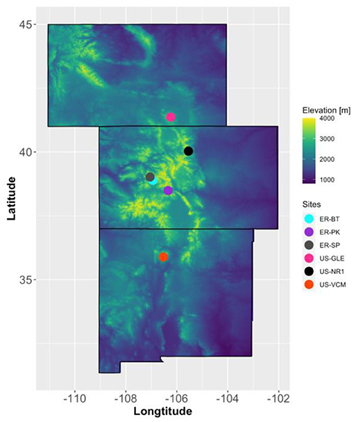
Figure 1. Geographical locations of the six sites selected in this study. ER-BT, ER-PK, and ER-SP represent Butte, Porphyry Creek, and Scofield Pass SNOTEL stations. US-GLE, US-NR1, and US-VCM are the three FLUXNET sites considered in this study.
In order to understand the influence of hydroclimate on ET dynamics over multiple years, we focused on data collected between 2005 and 2016, which captures the general temporal variability of ET dynamics at these sites. At the three FLUXNET sites (FLUXNET2015 Dataset), eddy covariance towers provided half-hourly direct measurements of meteorological forcing data, including air temperature, precipitation, and solar radiation, which were aggregated into daily scales. At the three SNOTEL sites in the East River Watershed, high quality meteorological forcing data were obtained from https://wcc.sc.egov.usda.gov/, including temperature and precipitation. We followed approaches proposed by Oyler et al. (2015) to filter potential systematic artifacts in air temperature data. Since solar radiation data are not available at these three SNOTEL sites, we integrated incident solar radiation from the DAYMET database (Thornton et al., 2017). DAYMET data was also used to replace any missing data. At US-VCM, meteorological forcing data from 2005 and 2007 and after the fire period were obtained from DAYMET. Table 1 provides a statistical summary of meteorological forcing attributes and climate Koeppen classification (Arnfield, 2017) at these six sites. The six sites considered in this study are representative of the Upper Colorado River Basin temperature and precipitation variability.

Table 1. Summary characteristics of the six sites selected in this study.
At the FLUXNET sites, ET data were calculated from the latent heat fluxes measured from eddy covariance towers. Community land models (CLM) were developed for calculating ET at both FLUXNET sites and SNOTEL sites in the East River Watershed (Tran et al., 2019). A comparison between ET estimated from CLM and direct measurements from the three FLUXNET sites is provided in the Supplementary Materials (Supplementary Figure 1, R2 >0.8, k > 0.94, p < 2.2e−10, MAE < 0.25 mm for all three sites), and supports the use of CLM ET estimates and their integration with direct flux measurements. Community land model simulated results were also used to append ET data at FLUXNET sites when data availability became limited. At US-VCM, we used the ET estimation from CLM to replace the post-fire dynamics after May 2013. Time series of ET after 2013 do not consider the effects caused by fire at US-VCM. CLM ET estimates were used for ER-BT, ER-SP, and ER-PK. Despite the high estimation accuracy of CLM models observed at FLUXNET sites, augmented ET data for FLUXNET sites and ET estimation from SNOTEL sites are subject to any conceptual model and parameter uncertainties inherited in CLM, however the use of CLM estimates does not restrict the applicability of our approaches.
The Palmer drought severity index (PDSI) estimates relative dryness of watersheds using temperature and precipitation data. Palmer drought severity index values have been reasonably successful in capturing long-term drought conditions. We obtained PDSI time series (monthly scale) at the six watersheds from Abatzoglou et al. (2018), which enabled us to quantify drought influence over subseasonal ET dynamics. We selected June-PDSI values to quantify fore-summer drought conditions; then classified droughts into the following categories, based on U.S. Drought Monitor classifications:
In this section, we start with introducing the concept of subseasonal regimes. The crux of subseasonal regime approach—Hidden Markov Model—is explained in section Hidden Markov Models. Hypothesis testing [e.g., analysis of variance (ANOVA) and Tukey's tests] is used to estimate the heterogeneity of meteorological forcing attributes and ET in both space and time and is presented in section ANOVA and Tukey's Test.
Subseasonal regimes represent the period of time that has distinguishable combinations of statistical characteristics—meteorological forcing attributes and ET-values—compared to other subseasonal regimes, which physically represent the duration and occurrence of subseasonal events, such as snow accumulation, snowmelt, growing season, monsoon season, and defoliation periods. The concept of subseasonal regime is developed to capture subseasonal variability in meteorological forcing variables and ET dynamics. Subseasonal regimes are determined statistically using the Hidden Markov Models (HMM) and the number of subseasonal regimes are optimized based on statistical metrics (e.g., Akaike information criterion and Bayesian information criterion). Figure 2 summarizes the steps to identify subseasonal regimes and use subseasonal regimes to analyze inter- and intra-annual variability of ET. The subseasonal regime approach depends on input data quality. Thus, the first step is to clean FLUXNET datasets and SNOTEL datasets and prepare necessary input parameters. Data QA/QC steps are necessary to ensure the input data quality and reduce errors in regime identifications and further analysis. Hidden Markov Model is the applied to statistically identify the subseasonal regimes for each site and each year. The number of subseasonal regimes is optimized statistically. In this study, five regimes were selected as it has the smallest Akaike information criterion and Bayesian information criterion.
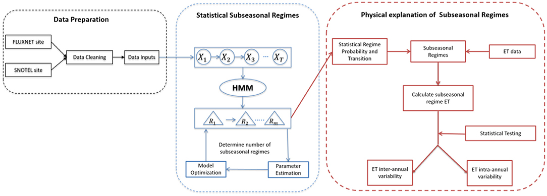
Figure 2. Schematic steps for the subseasonal regime approach.
Statistical regime probability and transition are then used to physically explain the impact of subseasonal events on ET dynamics. With subseasonal regimes being determined from the HMM, we define subseasonal cumulative ET (Ri ET) that represents the contribution of ET from each individual subseasonal regime to annual cumulative ET, as indicated in Equation (1), where ETRi is the regime-mean ET (mm/d) and durationRi represents the duration of subseasonal regime Ri in m unique subseasonal regimes.
Hypothesis testing methods, such as ANOVA and Tukey's test, are applied to further delineate the impacts of droughts on inter- and intra-annual variability of ET dynamics. The overall subseasonal regime approach holistically incorporates the onsets of multiple watershed dynamics and assess the impacts of fore-summer drought on the subseasonal variability of ET.
Hidden Markov Models is a statistical model in which the system being modeled is assumed to be a Markov process with unobserved (i.e., hidden) states. Among many other studies, HMM has been used to characterize mechanistic reaction networks of uranium transport in a contaminated aquifer (Chen et al., 2013), reconstruct streamflow (Bracken et al., 2014, 2016), and predict spatiotemporal variability in precipitation (Foufoula-Georgiou and Lettenmaier, 1987; Zucchini and Guttorp, 1991). Here we follow notations employed in Chen et al. (2013) and Zucchini and MacDonald (2009) to present a brief summary of HMM. For observed time series of hydroclimate attributes (Xt, t = 1, 2, …, T, i.e., air temperature, precipitation, and radiation), we define a subseasonal regime variable Rt, t = 1, 2, …, T, where Rt takes values from 1, 2, …, m, which represents m unique subseasonal regimes. The emission (output) probabilities are used to relate “subseasonal regimes” with the observed measurements (i.e., meteorological forcing attributes), and are modeled by state-dependent probability distributions:
A first-order Markov process has been assumed to represent the time series behavior of measurements and subseasonal regimes, which are presented as follows.
The transitional probability matrix denotes the probabilities of transitions between subseasonal regime i to subseasonal regime j, and are expressed as:
where R denotes a subseasonal regime determined from HMM. If k = j, then no transition of the subseasonal regimes occurs in the time domain. In order to estimate the unknown parameters, the likelihood function is derived, which is the joint conditional probability distribution of all the data given unknown parameters with the initial probability of unknown subseasonal regime. The unknown parameters (including subseasonal regimes) can be determined using the Expectation-Maximization algorithm. More details about deriving the likelihood function and the E-M algorithm can be found in Dempster et al. (1977) and Zucchini and Guttorp (1991). Additional resources on HMM can be found at Zucchini and MacDonald (2009). We used the package “depmixS4” in R developed by Visser and Speekenbrink (2010) for implementation.
In this study, we used air temperature, soil temperature, and radiation as inputs to HMM. In addition, a categorical variable (sn) that represents hydrological dynamics is also included as an input. The variable sn is determined based on the time series of air and soil temperature, as well as precipitation data. It provides a proxy for peak snow day, bareground day, and effective monsoon day, which represent the day with maximum snow depth, the first day of snow disappearance, and the first day that has monsoon precipitation >10 mm, respectively. sn provides indirect information about infiltration, vegetation growth, snowmelt timing, and start of monsoon season.
We assumed a Gaussian distribution for the emission probability for air temperature, soil temperature, and radiation inputs. Figure 3 displays hypothesized seasonal events, wherein we characterize any year into regimes of snow accumulation, snowmelt, growing season, monsoon season, and defoliation season. The onset of subseasonal events depicted by subseasonal regimes are selected based upon the mode of 1,000-HMM simulations with the optimal information criterion (Akaike, 1974; Schwarz, 1978).
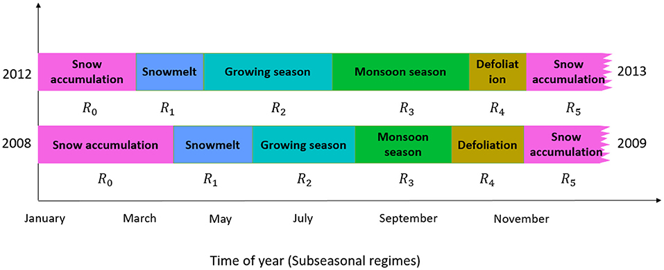
Figure 3. Example subseasonal regimes (Ri) within a year, which could include snow accumulation, snow melt, growing season, monsoon, and defoliation. Xi represents the data used to determine subseasonal regimes and follow a statistical distribution denoted by . are the mean and variance of Xi under specific subseasonal regimes, respectively.
We applied ANOVA to test the null hypothesis that the mean values of meteorological forcing attributes and ET from the six sites do not vary significantly. A test statistic (e.g., F-statistics) is calculated and used to calculate a p-value, which is compared to a preset significance level (0.05 in this study). When the p-value is smaller than the significance level, the null hypothesis is rejected. Rejecting the null hypothesis indicates that the differences in hydroclimate attributes and ET across different sites are unlikely to be random. Analysis of variance is not capable of identifying which location or which year is statistically different from the other locations or years when the null hypothesis is rejected. Hence, Tukey's test (Tukey, 1949) is also used to further determine pairwise differences across the six sites. This test is based on a studentized range distribution to determine whether or not to reject the null hypothesis. Failing to reject the null hypothesis indicates that the mean of the two pairs are not significantly different from each other. We also applied linear regression to determine the trends of meteorological forcing and ET over time under climate change. The slope coefficient represents the rate of change in attributes over years. A goodness of fit test is usually performed, together with linear regression, to determine if such a slope coefficient is statistically significant, which indicates whether the trend of meteorological forcing or ET dynamics is statistically significant under climate change.
In this section, we first present the spatial heterogeneity and temporal variability observed in meteorological forcing attributes and ET data across the sites selected in this study (section Non-linear Interactions Between Meteorological Forcing and ET Dynamics). Then we explore the characteristics of each subseasonal regime (section Characteristics of Subseasonal Regimes), including the underlying dominant processes in each subseasonal regime (section Intra-Annual Variability of ET). In section Timing and Duration of Subseasonal Regime as the key Controls for Subseasonal Cumulative ET and Annual ET, we provide an analysis of the subseasonal variability in ET through subseasonal cumulative ET based on subseasonal regimes. Section Linking Subseasonal Regimes With Dynamics Observed in the Physical Environment explains the linkage between subseasonal regimes and watershed dynamics observed in the physical environment. In section Assessing ET Inter-Annual Variability Through Identifying Regime-Based Contributions, the last section, we document how determination of subseasonal regimes can improve our understanding of subseasonal ET variability.
The six sites selected in this study cover a wide range of annual mean air temperatures, annual rain precipitation, annual snow precipitation, annual mean solar radiation, annual ET, and annual P-ET (Figure 4). We observed approximately a 5°C difference in the annual mean temperatures between US-VCM and US-GLE; a 500 mm difference in snow precipitation between US-VCM and US-GLE; and a 100 mm difference in rain precipitation between US-NR1 and ER-PK. Meteorological forcing attributes (e.g., precipitation, temperature, and radiation) across the sites exhibited much larger variability than did annual ET. Analysis of variance with annual ET data rejected the null hypothesis, which suggested that at least the mean of annual ET in one of the six sites was statistically different from the others. Tukey's test further indicated, with a 95% family-wise confidence level, that there were no statistical differences in annual ET between the following pairs: ER-SP and ER-BT, US-NR1 and ER-BT, US-VCM and ER-BT, US-NR1 and ER-SP, US-VCM and ER-SP, US-GLE and ER-PK, and US-VCM and US-NR1. Table 2 displays the results from the Tukey test on annual ET.
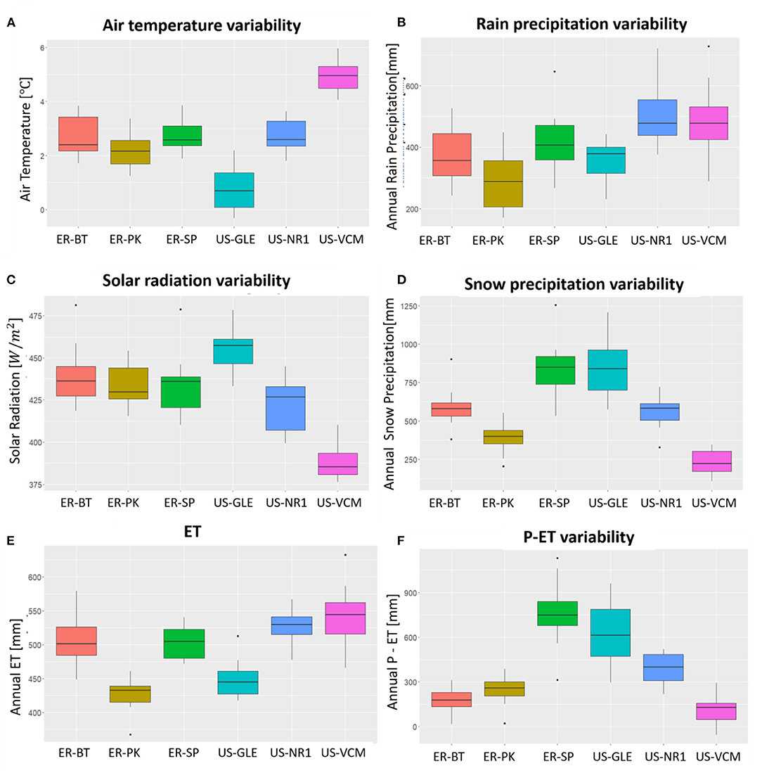
Figure 4. Spatial variability in attributes air temperature (A), rain precipitation (B), solar radiation (C), and snow precipitation (D) as well as ET (E) and P-ET (F) across the six sites.
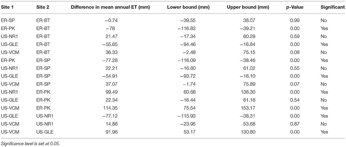
Table 2. Tukey's test result indicates differences in annual ET for certain pairs at family-wise 95% level.
The variability in meteorological forcing at tributes across these sites is influenced by their latitudes, elevation, and other local-scale factors. For example, we observed highest air temperature at US-VCM, followed by the three SNOTEL sites and US-NR1, with US-GLE having the lowest air temperature. On the other hand, maximum annual solar radiation was observed for US-GLE, followed by SNOTEL sites and US-NR1, with US-VCM as the lowest. Rain precipitation and snow precipitation across these six sites are complex. We observed greater rain precipitation at US-NR1 and US-VCM, whereas ER-PK had the relatively smallest annual rain precipitation. Largest snow precipitation was observed at US-GLE and ER-SP, whereas lowest snow precipitation generally occurred at US-VCM. Although these six sites are all located in the Colorado River Basin region, they span a wide range of latitudes, leading to significant differences in their energy inputs, as well as their precipitation inputs. Spatial variability in snow precipitation and total precipitation minus ET (P – ET) is also linked with energy inputs and latitudes, whereas we observed the greatest snow precipitation and P – ET at US-GLE, followed by US-NR1, with US-VCM having the lowest snow precipitation and P – ET. However, this relationship became much more complex when we further considered the three SNOTEL sites that have similar latitude. We observed similar annual snow precipitation between ER-SP and US-GLE; ER-BT and US-NR1; however, annual P – ET of ER-BT was closer to US-VCM. Despite significant differences in energy and precipitation patterns among these sites, we observed some similarity in the temporal distribution of annual ET between US-NR1 and US-VCM; ER-BT and ER-SP; and ER-PK and US-GLE. These findings emphasize the importance of exploring subseasonal variability when investigating controls on ET dynamics.
In this section, we present the statistical summary of meteorological forcing attributes determined for each subseasonal regime, and demonstrate the physical representation of each determined subseasonal regime and how dynamic changes in hydroclimate govern ET dynamics. With the proposed framework, six subseasonal regimes (R0–R5) that have distinct statistical characteristics in meteorological forcing attributes and ET were determined. Figure 5 presents the subseasonal regime-based distribution of air temperature (Figure 5A), solar radiation (Figure 5B), rain precipitation (Figure 5C), snow precipitation (Figure 5D), ET (Figure 5E), and net precipitation minus ET (Figure 5F) across all six sites and years considered.
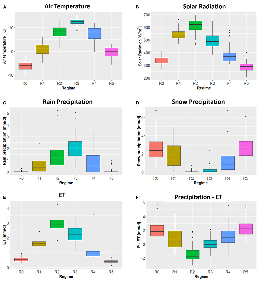
Figure 5. Summary of subseasonal regime-based characteristics of daily air temperature (A), solar radiation (B), rain precipitation (C), snow precipitation (D), ET (E), and precipitation minus ET (F) at all six sites in this study.
Starting in January, subseasonal R0 usually represents the snow accumulation period when the watershed is covered by snow, which has minimum temperature, minimum solar radiation, and minimum ET. The duration of R0 is largely controlled by snow precipitation and the effective accumulation of snow during the winter time. During R0, positive P – ET is observed. Because plants are lacking adequate light, temperature, and moisture conditions to grow, most of the snow precipitation is consumed by other processes rather than supporting plant growth and evapotranspiration. Toward the end of R0, as temperature reaches above the freezing point and solar radiation increases, R0 and R1 transition happens following the start of snowmelt. During R1, soil moisture supplied from melted snow supports nutrient transport in the subsurface (Sorensen et al., 2020). However, due to limited energy conditions (e.g., low air temperature), R1-based ET is still very small (~1.6 mm/d). Compared to R0 and R5, we observe a decrease in P – ET due to higher potential evaporation, resulting from increasing radiation inputs. Snow disappearance usually occurs at the end of R1; the bareground date is highly correlated with the day of R1-R2 transition. Duration of R1 is important, for it controls the amount of soil moisture from snowmelt that can be potentially used to support vegetation growth during the subsequent growing season. During R1, snowmelt water also contributes to groundwater and stream recharge. R2 and R3 correspond to the growing season, and experience greater variability in ET. R2 represents the period of time during which the watershed experiences maximum radiation, supporting vegetation growth. At the beginning of R2, the rate of vegetation growth is very high, owing to ambient soil moisture from snowmelt and radiation, where we observed an increase in ET. We observed the largest ET but the smallest P – ET in R2. With combinations of earlier snowmelt and later monsoon, decreases in R2-mean that ET occurs, which could lead to drought conditions (as described in section Assessing ET Inter-Annual Variability Through Identifying Regime-Based Contributions). The decreases in R2-mean that ET has been associated with fore-summer droughts (Sloat et al., 2015; Wainwright et al., 2020). Correspondingly, earlier R1–R2 transition (earlier snowmelt) is usually associated with small R2-mean ET. R2–R3 transition is controlled by the first effective monsoon, which greatly reduces the potential for drought conditions posed in R2. Compared to R2, R3 has the highest rain precipitation inputs, and these monsoon precipitation events provide additional water supply for ET that supports both plant transpiration and soil evaporation. With the increasing precipitation inputs, we observed that R3 P – ET fluctuates around 0, compared to −2 in R2. This result indicates that monsoon precipitation during R3 is necessary for plants to survive potential droughts.
The R3 and R4 transitions usually take place in late autumn and correspond to the defoliation period, when temperature and radiation is low. During this period, most plants are adapting to winter dynamics, and ET declines. Though rainfall precipitation still occurs in R4, this moisture input does not contribute to ET because of energy limiting conditions and limited plant productivity. During this period, we observed net positive P – ET, indicating the additional precipitation inputs do not entirely contribute to ET, as energy becomes the limiting factor. R4-R5 transition is triggered when temperature decreases to the freezing point. R5 marks the start of winter, when the ecosystem has minimum ET and extends to R0 in the following year until snowmelt initiates the transition to R1. Due to the limited plant functionality and evaporative demands, the overall contributions of ET from R4, R5, and R0 are very small compared to snowmelt, growing season, and monsoon subseasonal regime.
Within-regime cumulative ET, calculated based on subseasonal regimes, provides a quantitative approach for assessing intra-annual variability in ET dynamics under different subseasonal regimes over space and time. Figure 6 displays the within-regime cumulative ET based on the corresponding subseasonal regimes across the six sites determined in this study. Comparing within-regime cumulative ET enables the quantification of the contributions from each subseasonal regime to annual ET, while distinguishing the unique roles of these dynamics in controlling the intra-annual variability of ET. For example, at a 95% confidence interval for within-R2, cumulative ET at US-NR1 and US-VCM are 146 ± 18 and 120 ± 27 mm, which account for 29.8% ± 5% and 22.5% ± 5% of the total annual ET, respectively. Within R3, cumulative ET at US-NR1 and US-VCM are 172 ± 28 and 243 ± 44 mm, which accounts for 30.1% ± 5.5% and 41.0% ± 6% of the total annual ET, respectively. We also observed significant fluctuations in annual ET, within-regime ET, and regime durations across the six watersheds. For example, at US-NR1 and US-GLE, we have identified stronger contributions in annual ET from within-R0 and within-R1 ET, whereas within-R3 ET is significantly stronger at US-VCM than US-NR1 and US-GLE. Correspondingly, the longest duration of R3 was observed at US-VCM, whereas the longest duration of R1 occurs at US-GLE and US-NR1 (Supplementary Figure 2). These comparisons further distinguish the effects of regimes in regulating intra-annual variability of ET across these Rocky Mountain watersheds.
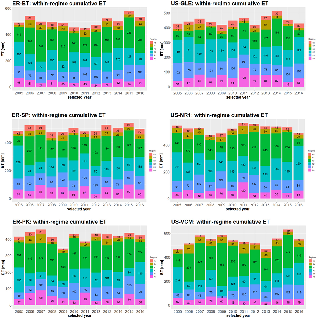
Figure 6. Subseasonal regime dependent partitioning of ET. Numbers within each column represents the amount of within-cumulative ET.
The dynamics of meteorological forcing attributes extend or shorten the duration of subseasonal regimes, and thus re-partition the annual cumulative ET into different subseasonal regimes. At ER-BT, within-R1 cumulative ET varies from 64 to 126 mm, and within-R2 cumulative ET varies from 77 to 187 mm where annual ET ranges from 446 mm (year 2011) to 579 mm (year 2015), during the years considered in this study. Through comparing the within-regime cumulative ET between 2011 and 2015, we determined that the differences in annual ET mainly resulted from within-R3 cumulative ET (124 vs. 233 mm). This indicates that adequate precipitation events and radiation inputs during the prolonged monsoon season in 2015 were the major drivers that led to the discrepancy in annual ET between 2011 and 2015, whereas ET dynamics during snowmelt periods, growing season, and other regimes are similar in these two years. These results indicate that differences in annual ET result from significant changes in sub-annual variability, whereas regime duration and transitions control the cumulative within-regime ET.
The magnitude of each subseasonal cumulative ET contributes to annual ET. Duration of subseasonal regimes and regime-mean ET control subseasonal cumulative ET, and thus influence the inter-annual variability of annual ET. Figure 7 presents the correlation between subseasonal regime duration and subseasonal cumulative ET. At each subseasonal regime, ET fluctuates around its regime-mean ET, which is relatively constant across various years and sites (k in Figure 7). Thus, the duration of subseasonal regimes is an important factor that leads to spatiotemporal variability in annual ET. Earlier snowmelt and extended fore-summer drought reshape the duration of subseasonal regimes, which further influences annual ET. Considering all years and sites, high correlations between regime durations and subseasonal cumulative ET were observed for R0–R5, which suggested an overall similarity in within-regime ET across the various sites. Regime-mean ET for R0–R5 is at 1.1, 1.5, 2.4, 2.7, 0.96 and 0.55 mm/d respectively. The prolonged durations of R2 and R3 increase the annual ET due to high regime-mean ET in R2 and R3. Adequately prolonged duration of R0 and R5, caused by higher snow precipitation and colder winter, increases R0 and R5 duration and delays R1-R2 transition and snowmelt, which provide sufficient water supply during high solar radiation, leading to an overall increase in annual ET. However, if the duration of R0 and R5 becomes excessive, it significantly decreases R2 and R3 duration and reduces annual cumulative ET. Further, ET dynamics also experience compensatory effects from these two subseasonal regimes (i.e., extended R2 and shortened R3 vs. shortened R2 and extended R3), leading to minor differences in annual ET (further explored in section Assessing ET Inter-Annual Variability Through Identifying Regime-Based Contributions). Finally, it can be noted that although the inferred k values (regime-mean ET) from regression between subseasonal cumulative ET and regime durations provide a statistical baseline for ET level, we observed a larger spread around the regression line, especially for R2 and R3. This spread indicates stronger site dependency linked to unique energy and moisture availability. Thus, characterizing the ET dynamics individually at each site is particularly needed during R2 and R3.
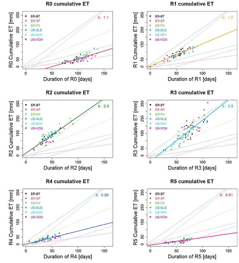
Figure 7. Correlation between subseasonal regime duration and regime cumulative ET. Colored points represent different sites. Colored lines are regression lines for each subseasonal regime between regime cumulative ET and subseasonal regime duration. k-values measure regime-mean ET [mm/day].
The regime-based approach is advantageous, because it holistically incorporates multiple watershed dynamics (e.g., the onset of snowmelt and monsoon, air temperature) to determine the intra-annual variability dynamics. Figure 8A presents the inter-annual variability of data-based indices, including bareground date, day of minimum net ecosystem exchange (NEE), day of maximum gradient in soil temperature, day of maximum soil moisture at US-NR1 supported by FLUXNET data, where R0–R1 and R1–R2 transition date were also used for comparison. In Figure 8B, we observed a high correlation between R0–R1, R1–R2 transition date and process-based indices, including bareground date, day of minimum NEE, day of maximum gradient in soil temperature, and day of maximum soil moisture. Though regime transition dates were identified statistically, they provided proxies for processes that are difficult to quantify over space and time. For example, date of R0–R1 transition is related to the start of snowmelt processes and infiltration into the subsurface. The R1–R2 transition date provides an integrated proxy of bareground date and start of vegetation growth with maximum soil moisture.

Figure 8. Coherence between hydrological indices, R0–R1, and R1–R2 transitions at US-NR1: (A) presents the annual series of bareground date (Bg_date), day of minimum net ecosystem exchange (NEE), day of maximum gradient in soil temperature (SoilT), day of maximum soil moisture (VWC), R0_R1 transition, and R1_R2 transition; (B) depicts the correlation plot among these variables.
We used the data at US-NR1 as an example to further illustrate the coherence between various observations in the physical environment and assessed how they're related to the timing of subseasonal regimes based on statistics. Supplementary Figure 3 presents the time series of snow water equivalent (SWE), ET, soil temperature, and soil water content of 2008 and 2012 at US-NR1. Significant consistency in all these processes was observed, including date of maximum snow depth, first day of snow disappearance (bareground date), and day of air and soil temperature above 0°C. This result indicates that changes in snow dynamics are correlated with changes in other dynamics, such as soil temperature and ET. Correlations in watershed dynamics have been reported in other studies. For example, (1) soil moisture dynamics and the timing of snowmelt are highly correlated (Harpold and Molotch, 2015); (2) dynamic changes in meteorological forcing also lead to temporal variations in ecosystem respiration and gross primary production (Knowles et al., 2016; Berryman et al., 2018); and (3) fore-summer drought occurrences are also highly linked with the timing of snowmelt and shifts in energy inputs (Sloat et al., 2015; Wainwright et al., 2020). Thus, regime-based approaches provide avenues for quantitatively unifying various influential processes to better evaluate ET dynamics.
Regime-based consideration of intra-annual variability of ET explains the seasonal driver of inter-annual variability of ET across sites. At ER-BT, earlier snowmelt led to approximately 3 weeks earlier R0–R1 transition in 2012 (75th day) compared to 2008 (99th day), where snowmelt did not start until April. R1–R2 transition is 2 weeks apart between 2008 (153th day) and 2012 (137th), due to different rates of snowmelt and the onset of snowmelt (Supplementary Figure 2). R2–R3 transition occurred at the 205th and 189th day in 2008 and 2012, respectively. The earlier R2–R3 transition in 2012 resulted from the earlier arrival of monsoon precipitation, which also relieved the effect of fore-summer drought. Correspondingly, significant differences in subseasonal cumulative ET between 2008 and 2012 were observed, including a +27 mm differences in R0 cumulative ET, −28 mm differences in R1 cumulative ET, +53 mm differences in R2 cumulative ET and a – 31 mm difference in R3 cumulative ET. These results showed that the intra-annual variability of ET can vary strongly between 2 years, while annual ET can remain quite similar. Annual ET in 2008 and 2012 was equal to 493 and 474 mm, respectively. This result indicates that annual ET differences are compensated by different subseasonal cumulative ET that is controlled by different seasonal drivers. Ambient moisture from later snowmelt contributed more ET during snowmelt and the growing season in 2008, whereas monsoon precipitation played a more essential role in sustaining ET and plant growth in 2012.
At the other Colorado sites (i.e., ER-SP, ER-PK, and US-NR1) and US-VCM, we observed a similarly early R0–R1 and R1–R2 transition in 2012 compared to 2008. However, at US-GLE, R0–R1 and R1–R2 transitions were not the same as observed at the Colorado sites. US-GLE had longer R0 and R1 durations, likely due to its higher latitude and more accumulation of snow during winter, which also caused later R0–R1 and R1–R2 transitions compared to lower latitude sites. At US-GLE, the annual ET was 439 mm for 2008 and 417 mm for 2012. Though the R0–R1 transition between 2008 and 2012 was not as different as at the Colorado sites, different contributions from within-R2 and within-R3 ET resulted in overall differences in annual ET. Similarly, at US-VCM, differences in annual ET between 2008 and 2012 were largely caused by R2 cumulative ET (145 mm in 2008 vs. 95 mm in 2012).
Regime-based approaches further delineate fore-drought impacts on inter- and intra-annual variability of ET dynamics. Considering all sites and years, we observed no significant relationships between annual ET and fore-summer drought occurrence. For example, annual ET differences between severe drought years and normal/wet years across all sites range from−89 to 63 mm (Supplementary Table 1; Supplementary Figure 4). However, significant differences in annual P – ET between normal/wet years and extreme/exceptional drought years across all sites were observed and expected (Supplementary Table 2; Supplementary Figure 4). In addition, Supplementary Figure 4 presents the distribution of regime-mean P – ET across different drought levels. During R1, excessive snow precipitation distinguished normal/wet years from other dry years in P – ET; however, R1 ET is not significantly different in normal/wet and dry years, as moisture is not yet the limiting factor. Snowmelt water is the major contributor for R2 ET. We found slightly greater R2 ET in normal/wet years compared to other dry years that experience fore-summer droughts, and a significant decline in R2 ET was observed for exceptional drought years. During the exceptional dry years, both P and ET were very small, and P – ET is closer to 0. In R3, P – ET across drought conditions fluctuates around 0, indicating the relative balance between monsoon precipitation and ET. These results indicate that excessive snow precipitation during normal/wet years is not effectively contributing to ET and is more important for other hydrological pathways (e.g., streamflow). During drought years, additional precipitation (especially monsoon) plays a vital role in restoring ET and compensating for the loss of ET during the preceding dry periods. Carroll et al. (2020) found that drought conditions modify monsoon precipitation's contributions to ET and streamflow. Their study suggested that monsoon precipitation is mainly effective in moistening dry soil and sustaining ET at lower subalpine forests during dry years, while being the primary contributor to streamflow generation under normal/wet year conditions. Timing and location of monsoon water input with respect to energy and water availability remain as the key factors for ET and streamflow generation during these periods. At the Sierra Nevada critical zone, Bales et al. (2018) also discovered that trees can access groundwater during drought conditions, leading to minor fluctuations in ET compared to normal/wet years. Though annual ET may remain similar across different drought conditions, contributions to ET from different regimes can change significantly, indicating shifts in the dominant drivers for subseasonal ET dynamics. With the projected earlier snowmelt (Barnhart et al., 2016) and increasing uncertainties in North American monsoon (Notaro and Zarrin, 2011) in the Rocky Mountain regions, we believe regime-based approaches can better quantify these changes in meteorological conditions, as well as provide us with informative insights to better quantify climate change's influence on ET dynamics.
In this study, we developed the framework of subseasonal regimes to better characterize the intra-annual variability of ET dynamics at mountainous watersheds. With this method, we were able to delineate subseasonal regimes associated with snow, snowmelt, growing season, monsoon, and defoliation. Our proposed framework of subseasonal regimes has the advantage of being able to quantitatively distinguish the distinct contribution from intra-annual dynamics to inter-annual variability, as well as assess the contribution of seasonal events important for water and energy resources management. Our approach provides a unique perspective, delineating how watershed processes (including droughts) control the intra-annual variability of ET.
Regime-mean ET is relatively constant across all years and the six watersheds. Subseasonal regime duration and occurrences of regime transition are the pivotal factors that lead to the magnitude of annual cumulative ET. Our study also suggests that the subseasonal variability of ET indicated by subseasonal regimes is as significant as or even greater than the inter-site and inter-annual variability of ET along the Colorado River Basin regions. Quantifying subseasonal variability enables insights regarding the cause and effect between long-term climate change trends and ET dynamics.
We also investigated how drought conditions affect both the inter-annual and intra-annual variability of ET dynamics. Our results suggest annual ET variability remains small considering all six watersheds across different drought levels, whereas annual P – ET differs significantly between normal/wet years and severe drought years. Snowmelt water is necessary for ET dynamics during R2 for both normal/wet and dry years, but earlier snowmelt and occurrence of exceptional fore-summer drought can lead to significant decline in R2 ET. The role of monsoon precipitation also changes between normal/wet years and dry years. In relatively dry years, monsoon precipitation is effectively sustaining ET (especially R3 ET), whereas excessive precipitation is less influential for ET during energy-limiting conditions. These results suggest the necessity and value of regime-based approaches to better evaluate how watershed processes and dynamic changes in drought conditions influence the inter-annual and intra-annual variability of ET dynamics.
The subseasonal-regimes construct described here is mainly based on certain meteorological forcing attributes. We note that incorporation of additional informative parameters, along with the right choice of statistical distribution for the emission probability (such as NDVI as a proxy for plant status or soil moisture as a proxy for subsurface moisture stress), could further help to delineate subseasonal regimes that cover additional aspects of watershed processes. Though not assessed in this current study, we believe that the subseasonal regime approach is sufficiently general and extendable to quantify the subseasonal variability of other hydrological and ecological processes at other sites.
The datasets presented in this study can be found in online repositories. The names of the repository/repositories and accession number(s) can be found in the article/Supplementary Material.
All authors listed have made a substantial, direct, and intellectual contribution to the work and approved it for publication.
We acknowledge support from the Jane Lewis Fellowship of University of California, Berkeley and the U.S. Department of Energy, Office of Science, Office of Biological and Environmental Research, Watershed Function SFA under Contract No. DE-AC02-05CH11231 to Lawrence Berkeley National Laboratory.
The authors declare that the research was conducted in the absence of any commercial or financial relationships that could be construed as a potential conflict of interest.
All claims expressed in this article are solely those of the authors and do not necessarily represent those of their affiliated organizations, or those of the publisher, the editors and the reviewers. Any product that may be evaluated in this article, or claim that may be made by its manufacturer, is not guaranteed or endorsed by the publisher.
The Supplementary Material for this article can be found online at: https://www.frontiersin.org/articles/10.3389/frwa.2021.739131/full#supplementary-material
Abatzoglou, J. T., Dobrowski, S. Z., Parks, S. A., and Hegewisch, K. C. (2018). TerraClimate, a high-resolution global dataset of monthly climate and climatic water balance from 1958–2015. Sci. Data 5, 1–12. doi: 10.1038/sdata.2017.191
Akaike, H. (1974). A new look at the statistical model identification. IEEE Trans. Automat. Contr. 19, 716–723. doi: 10.1109/TAC.1974.1100705
Arnfield, J. (2017). Köppen climate classification climatology. Encyclopedia Britannica (accessed August 04, 2017).
Bales, R. C., Goulden, M. L., Hunsaker, C. T., Conklin, M. H., Hartsough, P. C., O'Geen, A. T., et al. (2018). Mechanisms controlling the impact of multi-year drought on mountain hydrology. Sci. Rep. 8, 1–8. doi: 10.1038/s41598-017-19007-0
Barnhart, T. B., Molotch, N. P., Livneh, B., Harpold, A. A., Knowles, J. F., and Schneider, D. (2016). Snowmelt rate dictates streamflow. Geophys. Res. Lett. 43, 8006–8016. doi: 10.1002/2016GL069690
Berryman, E. M., Vanderhoof, M. K., Bradford, J. B., Hawbaker, T. J., Henne, P. D., Burns, S. P., et al. (2018). Estimating soil respiration in a subalpine landscape using point, terrain, climate, and greenness data. J. Geophys. Res. Biogeosci. 123, 3231–3249. doi: 10.1029/2018JG004613
Blankinship, J. (2014). Snowmelt timing alters shallow but not deep soil moisture in the Sierra Nevada. Water Resour. Res. 50, 1448–1456. doi: 10.1002/2013WR014541
Bracken, C., Rajagopalan, B., and Woodhouse, C. (2016). A Bayesian hierarchical nonhomogeneous hidden Markov model for multisite streamflow reconstructions. Water Resour. Res. 52, 7837–7850. doi: 10.1002/2016WR018887
Bracken, C., Rajagopalan, B., and Zagona, E. (2014). A hidden Markov model combined with climate indices formultidecadal streamflow simulation. Water Resour. Res. 50, 1–11. doi: 10.1002/2014WR015567
Budyko, M. I. (1961). The heat balance of the earth's surface. Sov. Geogr. 2, 3–13. doi: 10.1080/00385417.1961.10770761
Carroll, R. W., Gochis, D., and Williams, K. H. (2020). Efficiency of the summer monsoon in generating streamflow within a snow-dominated headwater basin of the Colorado River. Geophys. Res. Lett. 47:e2020GL090856. doi: 10.1029/2020GL090856
Chen, J., Hubbard, S. S., and Williams, K. H. (2013). Data-driven approach to identify field-scale biogeochemical transitions using geochemical and geophysical data and hidden Markov models: development and application at a uranium-contaminated aquifer. Water Resour. Res. 49, 6412–6424. doi: 10.1002/wrcr.20524
Condon, L. E., and Maxwell, R. M. (2019). Simulating the sensitivity of evapotranspiration and streamflow to large-scale groundwater depletion. Sci. Adv. 5, eaav4574. doi: 10.1126/sciadv.aav4574
Dempster, A. P., Laird, N. M., and Rubin, D. B. (1977). Maximum likelihood from incomplete data via the EM algorithm. J. R. Stat. Soc. B 39, 1–38. doi: 10.2307/2984875
Ernakovich, J. G., Hopping, K. A., Berdanier, A. B., Simpson, R. T., Kachergis, E. J., Steltzer, H., et al. (2014). Predicted responses of arctic and alpine ecosystems to altered seasonality under climate change. Glob. Chang. Biol. 20, 3256–3269. doi: 10.1111/gcb.12568
Fatichi, S., and Ivanov, V. Y. (2014). Interannual variability of evapotranspiration and vegetation productivity. Water Resour. Res. 50, 3275–3294. doi: 10.1002/2013WR015044
Foster, L. M., Bearup, L. A., Molotch, N. P., Brooks, P. D., and Maxwell, R. M. (2016). Energy budget increases reduce mean streamflow more than snow-rain transitions: using integrated modeling to isolate climate change impacts on Rocky Mountain hydrology. Environ. Res. Lett. 11, 044015. doi: 10.1088/1748-9326/11/4/044015
Foufoula-Georgiou, E., and Lettenmaier, D. P. (1987). A Markov renewal model for rainfall occurrences. Water Resour. Res. 23, 875–884. doi: 10.1029/WR023i005p00875
Frank, J. M., Massman, W. J., Ewers, B. E., Huckaby, L. S., and Negrón, J. F. (2014). Tree mortality from spruce bark beetles. J. Geophys. Res. Biogeosci. 119, 1195–1215. doi: 10.1002/2013JG002597
Harpold, A., and Molotch, N. P. (2015). Sensitivity of soil water availability to changing. Geophys. Res. Lett. 42, 8011–8020. doi: 10.1002/2015GL065855
Hubbard, S. S., Williams, K. H., Agarwal, D., Banfield, J., Beller, H., Bouskill, N., et al. (2018). The East River, Colorado, Watershed: a mountainous community testbed for improving predictive understanding of multiscale hydrological–biogeochemical dynamics. Vadose Zone J. 17. doi: 10.2136/vzj2018.03.0061
Immerzeel, W. W., Lutz, A. F., Andrade, M., Bahl, A., Biemans, H., Bolch, T., et al. (2019). Importance and vulnerability of the world' s water towers. Nature 577, 1–43. doi: 10.1038/s41586-019-1822-y
Knowles, J. F., Blanken, P. D., and Williams, M. W. (2016). Wet meadow ecosystems contribute the majority of overwinter soil respiration from snow-scoured alpine tundra. J. Geophys. Res. G Biogeosci. 121, 1118–1130. doi: 10.1002/2015J. G.003081
Litvak, M. (2016). AmeriFlux BASE US-Vcm Valles Caldera Mixed Conifer, Ver. 18-5. AmeriFlux AMP. doi: 10.17190/AMF/1246121
Monson, R. K., Turnipseed, A. A., Sparks, J. P., Harley, P., Scott-denton, L. E., Sparks, K., et al. (2002). Carbon sequestration in a high-elevation, subalpine forest. Glob. Chang. Biol. 8, 459–478. doi: 10.1046/j.1365-2486.2002.00480.x
Notaro, M., and Zarrin, A. (2011). Sensitivity of the North American monsoon to antecedent Rocky Mountain snowpack. Geophys. Res. Lett. 38, 17403. doi: 10.1029/2011GL048803
Oyler, J. W., Dobrowski, S. Z., Ballantyne, A. P., Klene, A. E., and Running, S. W. (2015). Artificila amplification of warming trends across the mountains of the western United States. Geophys. Res. Lett. 42, 153–161. doi: 10.1002/2014GL062803
Rauscher, S. A., Pal, J. S., Diffenbaugh, N. S., and Benedetti, M. M. (2008). Future changes in snowmelt-driven runoff timing over the western US. Geophys. Res. Lett. 35, L16703. doi: 10.1029/2008GL034424
Schwarz, G. (1978). Estimating the dimension of a model. Ann. Stat. 6, 461–464. doi: 10.1214/aos/1176344136
Sloat, L. L., Henderson, A. N., Lamanna, C., and Enquist, B. J. (2015). The effect of the foresummer drought on carbon exchange in subalpine meadows. Ecosystems 18, 533–545. doi: 10.1007/s10021-015-9845-1
Sorensen, P. O., Beller, H. R., Bill, M., Bouskill, N. J., Hubbard, S. S., Karaoz, U., et al. (2020). The snowmelt niche differentiates three microbial life strategies that influence soil nitrogen availability during and after winter. Front. Microbiol. 11, 871. doi: 10.3389/fmicb.2020.00871
Stocker, T. F., Qin, D., Plattner, G. K., Tignor, M. M. B., Allen, S. K., Boschung, J., et al. (2013). Climate Change 2013 The Physical Science Basis. Contribution of Working Group I to the Fifth Assessment Report of the Intergovernmental Panel on Climate Change [Stocker, T.F., D. Qin, G.-K. Plattner, M. Tignor, S.K. Allen, J. Boschung, A. Nauels, Y. Xia, V. Bex and P.M. Midgley (eds.)]. (Cambridge; United Kingdom; New York, NY: Cambridge University Press), p. 1535.
Thornton, P. E., Thornton, M. M., Mayer, B. W., Wei, Y., Devarakonda, R., Vose, R. S., et al. (2017). Daymet: Daily Surface Weather Data on a 1-km Grid for North America, Version 3. Oak Ridge, TN: DAAC.
Tran, A. P., Rungee, J., Faybishenko, B., Dafflon, B., and Hubbard, S. S. (2019). Assessment of spatiotemporal variability of evapotranspiration and its governing factors in a mountainous watershed. Water 11, 243. doi: 10.3390/w11020243
Tukey, J. W. (1949). Comparing individual means in the analysis of variance. Biometrics 5, 99–114. doi: 10.2307/3001913
Visser, I., and Speekenbrink, M. (2010). depmixS4: an R package for Hidden Markov models. J. Stat. Softw. 36, 1–21. doi: 10.18637/jss.v036.i07
Viviroli, D., Dürr, H. H., Messerli, B., Meybeck, M., and Weingartner, R. (2007). Mountains of the world, water towers for humanity: typology, mapping, and global significance. Water Resour. Res. 43, 1–13. doi: 10.1029/2006WR005653
Wainwright, H. M., Steefel, C., Trutner, S. D., Henderson, A. N., Nikolopoulos, E. I., Wilmer, C. F., et al. (2020). Satellite-derived foresummer drought sensitivity of plant productivity in Rocky Mountain headwater catchments: spatial heterogeneity and geological-geomorphological control. Environ. Res. Lett. 15, 084018. doi: 10.1088/1748-9326/ab8fd0
Zeng, R., and Cai, X. (2015). Assessing the temporal variance of evapotranspiration considering climate and catchment storage factors. Adv. Water Resour. 79, 51–60. doi: 10.1016/j.advwatres.2015.02.008
Zeng, R., and Cai, X. (2016). Climatic and terrestrial storage control on evapotranspiration temporal variability: analysis of river basins around the world. Geophys. Res. Lett. 43, 185–195. doi: 10.1002/2015GL066470
Zhang, D., Liu, X., Zhang, Q., Liang, K., and Liu, C. (2016). Investigation of factors affecting intra-annual variability of evapotranspiration and streamflow under different climate conditions. J. Hydrol. 543, 759–769. doi: 10.1016/j.jhydrol.2016.10.047
Zhang, L., Potter, N., Hickel, K., Zhang, Y., and Shao, Q. (2008). Water balance modeling over variable time scales based on the Budyko framework - model development and testing. J. Hydrol. 360, 117–131. doi: 10.1016/j.jhydrol.2008.07.021
Zucchini, W., and Guttorp, P. (1991). A Hidden Markov model for space-time precipitation. Water Resour. Res. 27, 1917–1923. doi: 10.1029/91WR01403
Keywords: evapotranspiration, intra-annual variability, climate change, statistics, Colorado River Basin
Citation: Chen J, Dafflon B, Wainwright HM, Tran AP and Hubbard SS (2022) A Subseasonal Regime Approach for Assessing Intra-annual Variability of Evapotranspiration and Application to the Upper Colorado River Basin. Front. Water 3:739131. doi: 10.3389/frwa.2021.739131
Received: 10 July 2021; Accepted: 21 December 2021;
Published: 13 January 2022.
Edited by:
Subimal Ghosh, Indian Institute of Technology Bombay, IndiaReviewed by:
Eswar Rajasekaran, Indian Institute of Technology Bombay, IndiaCopyright © 2022 Chen, Dafflon, Wainwright, Tran and Hubbard. This is an open-access article distributed under the terms of the Creative Commons Attribution License (CC BY). The use, distribution or reproduction in other forums is permitted, provided the original author(s) and the copyright owner(s) are credited and that the original publication in this journal is cited, in accordance with accepted academic practice. No use, distribution or reproduction is permitted which does not comply with these terms.
*Correspondence: Jiancong Chen, bmlnZWxfY2hlbjE5OTNAYmVya2VsZXkuZWR1
Disclaimer: All claims expressed in this article are solely those of the authors and do not necessarily represent those of their affiliated organizations, or those of the publisher, the editors and the reviewers. Any product that may be evaluated in this article or claim that may be made by its manufacturer is not guaranteed or endorsed by the publisher.
Research integrity at Frontiers
Learn more about the work of our research integrity team to safeguard the quality of each article we publish.