 Amin Ganjidoost
 Mark A. Knight1
- 1Department of Civil and Environmental Engineering, University of Waterloo, Waterloo, ON, Canada
- 2Department of Earth and Environmental Sciences, University of Waterloo, Waterloo, ON, Canada
This study develops an implementation framework for asset management strategic planning of water distribution networks to meet sustainable infrastructure, socio-political, and financial targets over the life cycle of the infrastructure. The proposed framework is comprised of three decision-making layers: (1) Visions and Values, (2) Function, and (3) Performance. The asset management strategy framework is implemented and validated by demonstrating functionality and value by using data from three water utilities in Canada. The Visions and Values layer is set to meet the needs of the water utilities' stakeholders. The Function layer uses an advanced system dynamics model to simulate and forecast the system's future behavior. The Performance layer benchmarks, compares, and graphically illustrates the situation and performance of water utilities against each other regardless of their size. Benchmarking results indicate that all three water utilities can sustainably meet the strategic targets established in the Visions and Values layer of the asset management strategy over the benchmarking period. The impact of the desired cash reserve on infrastructure and financial benchmarking performance indicators is also investigated to explore the “optimal” combination of allowable fee-hike and rehabilitation rates using the contour plots developed over the benchmarking period. The results indicate that the optimal combinations of allowable fee-hike of ~8% per year and rehabilitation rate of 1.3% per year along with a 1–4% cash reserve, depends on the network condition, will allow water utilities to have sufficient funds to meet their strategic targets. The performance modeling and simulation approach presented in this study represents a powerful tool for other utilities to develop optimal strategic and operational plans for their networks and thus better service to their stakeholders.
Introduction
Asset Management is the “coordinated activity of an organization to realize value from assets” (British Standard Institution., 2014). Asset Management involves “the balancing of costs and benefits, and risks and opportunities against the desired performance of assets, to achieve the organizational objectives” (British Standard Institution., 2014). It is argued that businesses have been able to increase their performance through adopting a systematic asset management approach (Lloyd, 2010).
Three interconnected decision-making layers for asset management strategy are identified as: (1) the outer circle (to find out “Where do we want to go?”); (2) the inner circle (to find out “How do we get there?”); and (3) the core circle (to find out “How are we doing?”) (Lloyd, 2010). The outer circle is the strategic level of decision-making that looks at the Visions and Values of an organization; the inner circle looks at the organization itself to find out how it is structured and operates to achieve its Vision and Values (i.e., the outer circle); and finally, the focal point of the decision-making (i.e., the core circle) monitors the achievement of the organization's visions and reinforces its values (Lloyd, 2010).
Efforts have been made to develop decision-support tools using system dynamics (SD) for asset management of water distribution and wastewater collection networks (Rehan et al., 2013, 2014a). These SD models are implemented for water distribution network (Rehan et al., 2015) and wastewater collection network (Rehan et al., 2014b) to find out (1) “Where do we want to go?” and (2) “How do we get there?.” The Rehan et al. (2013, 2015). SD models for strategic asset management of water distribution networks had some limitations, as described in section Water Distribution System Dynamics Model, such as the incomplete specification of fixed vs. variable revenue streams, lack of scaling the model to create an independent model for other utilities and assuming a constant price elasticity of demand for the utility's customers.
Ganjidoost et al. (2018) developed a series of normalized and time-integrated water and wastewater benchmarking performance indicators (BPI's) that conform to the four themes of the strategic target, policy lever, sustainability, and life cycle. The proposed BPI's enable water utilities to find out “How they are/will be doing?,” and hence pursue the best decision-making policies and management practices for sustainable long-term solutions. BPI's were grouped into three categories of infrastructure, socio-political, and financial that will allow water utilities with different attributes, to compare their performance against one another, and their own strategic targets. Table 1 provides a detailed description of BPI's for water distribution networks developed by Ganjidoost et al. (2018). All variables are time-varying to facilitate forecasting the BPI's over the asset life cycle. Those denoted as x(t) track system behavior instantaneously at the time “t,” while those denoted as X(T) are time-integrated to capture aggregate system behavior over the benchmarking period “T.” Ganjidoost et al. (2018) demonstrated the application of four BPI's to three water distribution networks to benchmark and compare system behavior over a 100-year benchmarking period using the Rehan et al. (2013)'s system dynamics model. It is found that the analyzed BPI's can improve stakeholders' understanding, support operational decisions, and thus improve performance over time. However, the case study presented by Ganjidoost et al. (2018) was limited to only four BPI's.
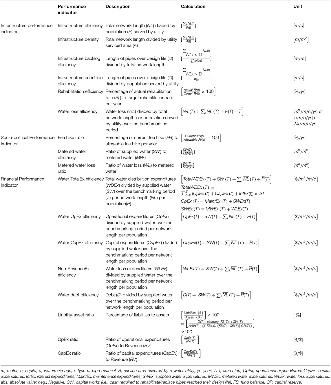
Table 1. Benchmarking performance indicators for water distribution networks—adopted from Ganjidoost et al. (2018).
This study develops an implementation framework for asset management strategic planning of water distribution networks by advancing Rehan et al. (2013)' SD model and implementing all water BPI's developed by Ganjidoost et al. (2018) to quantify the current and future performance of three water utilities in Southern Ontario, Canada.
Implementation Framework of Asset Management Strategy
An implementation framework is developed for the asset management strategy of water distribution networks comprised of three interconnected decision-making layers: “Visions and Values,” “Function,” and “Performance,” as shown in Figure 1. The Visions and Values layer conforms to the four themes: strategic target, policy lever, sustainability, and life cycle, as described by Ganjidoost et al. (2018). Function layer is advances made to Rehan et al. (2013, 2015) system dynamics model to fully answer the question of “How does the water utility achieve its Visions and Values?.” Then, the outputs of the advanced SD model are used to apply the entire set of BPI's developed by Ganjidoost et al. (2018) for the water distribution network to evaluate the total system's performance (i.e., the Performance layer). A good asset management practice involves the utility's stakeholders in its decision-making layers. Four key stakeholders for a water utility are (1) utility managers and employees, (2) customers (or community), (3) regulators, and (4) investors, as depicted in Figure 1. Utility managers and employees are involved in all three decision-making layers of asset management strategy. Customers and regulators are engaged in the Visions and Values layer of decision making, where the utility's strategic targets and policy levers controlling these targets are established. Investors desire to have access and evaluate the utility's outcomes (i.e., the Performance layer) to ensure an adequate return on their investments.
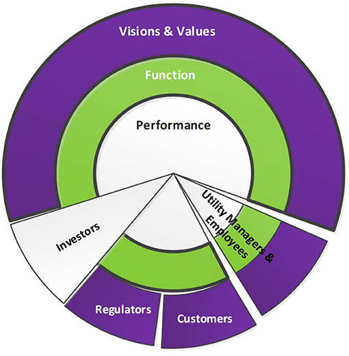
Figure 1. The utility key stakeholders' level of engagement in decision-making layers of asset management strategy: (1) Visions and Values, (2) Function, and (3) Performance.
The function and merit of the proposed implementation framework for the asset management strategy of water distribution networks are validated using data from three water utilities in Southern Ontario, Canada. The strategic targets and policy levers controlling these targets are established in the Visions and Values layer. The function layer uses an advanced system dynamics model to simulate and forecast each water utility's performance over their 100-year life cycle. The performance layer applies the entire set of water-related BPI's developed by Ganjidoost et al. (2018) to benchmark three independent water utilities' performance and demonstrate their use. This study is limited to linear water distribution pipelines.
Visions and Values Layer
The Visions and Values layer is set per the established concepts of strategic targets, policy levers, sustainability, and life cycle, as Ganjidoost et al. (2018) noted. Water utilities seeking to meet their Visions and Values should first set strategic targets, as indicated in Table 2, and then adjust policy levers, as noted in Table 3, to sustainably maintain these targets over the life cycle of the infrastructure. This layer of decision-making is intended to meet stakeholders' needs and comply with mandated legislation.
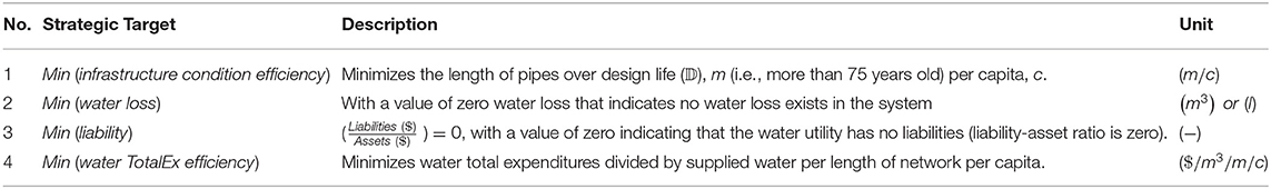
Table 2. Strategic targets for asset management strategy of water distribution network.
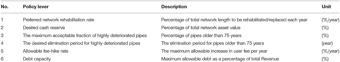
Table 3. Policy levers for asset management strategy of water distribution network.
Function Layer
The Function layer uses the advanced system dynamics model of this study, as presented in section Water Distribution System Dynamics Model, to achieve the stated Visions and Values of the water utility. The system dynamics model explicitly models the feedback mechanisms among various components of the water distribution network. The outputs of the advanced system dynamics model are used to simulate and forecast the future performance of the system.
Performance Layer
Ganjidoost et al. (2018) developed three groups of BPI for the water distribution network. These indicators are grouped into (1) infrastructure, (2) socio-political, and (3) financial. The BPI's are normalized to allow water utilities to benchmark themselves against each other locally, regionally and nationally, regardless of their size (see Table 1).
Water Distribution System Dynamics Model
A review of the Rehan et al. (2013, 2015) system dynamics models reveals some limitations associated with their model, such as the incomplete specification of fixed vs. variable revenue streams. To simulate and benchmark the three water utilities described in section Asset Management Strategy Implementation, the system dynamics model developed by Rehan et al. (2013) is further extended to achieve the stated Visions and Values of the water utility. The basic building blocks for SD models are stocks, flows (inflow/outflow), converters, and connectors, as depicted in Figure 2.
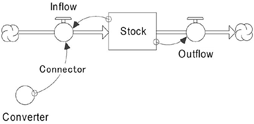
Figure 2. Building blocks of System Dynamics model.
Stocks represent accumulations, both physical and non-physical—for example, inventory of pipes and a customer's level of satisfaction. Flows represent activities or actions and are flow rates into, inflow, and out of, outflow, of a stock between the initial time t0 and the current time t. They transport quantities and can change instantaneously. The relationship between stocks and flows is represented as follow:
Connectors carry information to serve as inputs for decisions or actions. Converters are containers for performing algebra; they house graphical and built-in functions. The advanced system dynamics model for water distribution networks is comprised of three sectors: (1) infrastructure, (2) finance, and (3) socio-political.
Infrastructure Sector
The infrastructure sector represents the inventory of water distribution pipes. The American Water Works Association describes water distribution pipes as “pipelines that distribute water around a community” (AWWA, 2010). The physical condition of water distribution networks is simulated over a 100-year planning horizon, as shown in Figure 3. This study creates an infrastructure sector model for each independent water utility to represent each inventory of water mains. Due to the lack of condition assessment data obtained from the three case utilities, the degradation rate was assumed to exponentially increases as pipes aging (Ganjidoost et al., 2015a). This was only assumed to demonstrate the application of the model under identical assumptions for all three case utilities to benchmark their behavior over the simulation period. It should be noted that the forecasting feature of the SD model provides a good indication for utility stakeholders to collect more information on the actual structural health of assets and increase the accuracy of the long-term capital plans. Each stock in the infrastructure sector representing the length of pipes based on the material and age in each condition group (for example, Stock “CI 0 to 24”) can be updated and reconfigured upon the availability of actual condition assessment data.
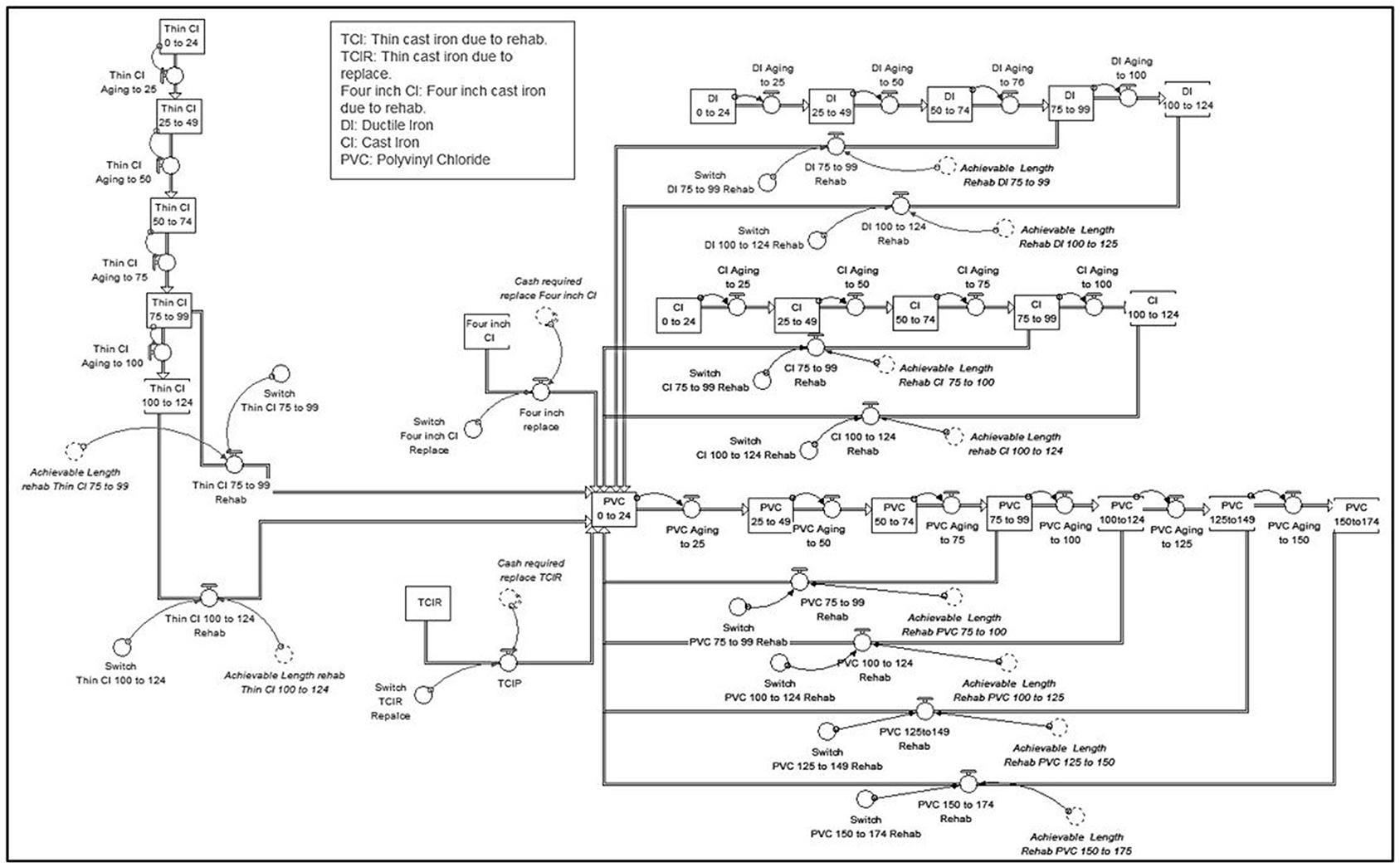
Figure 3. Infrastructure sector of the advanced system dynamic model in Stella®.
Finance Sector
The finance section describes the network's financial condition and includes Revenue, Expenditures, Fund Balance, Water Fee, etc., shown in Figure 4. The Revenue is the water utility's income that is measured in terms of variable and fixed fees. The Fund Balance is the difference between the total income and total expenditures of the network in dollars value. The Water Fee is the amount of currency ($/m3) that a water utility charges its customers to pay the expenses associated with the water services.

Figure 4. Finance sector of the advanced system dynamic model in Stella®.
The expenditures related to water utility services to provide potable water to customers are restricted to only “variable costs” in the Rehan et al. (2013) system dynamics model. However, the water utility customers are required to pay for the costs associated with the supplied water based on water consumption volume (Equation 2).
where WD Water Distribution; VC Variable Cost ($); Wf Water Fee ($/m3); MW Metered Water (m3); t time; cc classes of customers include residential, commercial and institutional.
They also need to pay a fixed cost for the services provided to them regardless of the amount of consumed water which is typically measured according to the size of service connections (pipe's diameter). The service connection delivers the treated water to each household (Equation 3).
where, FC Fixed Cost ($); d diameter of service connection for d = 15 mm, 19 mm, …, N; N maximum diameter of service connection; WSC Water Service Charges ($); NSC number of service connection.
This study incorporates fixed water service charges into the total revenue calculations from the customers (Equation 4). Therefore, the New Revenue (RV) in the advanced system dynamics model is measured as the sum of consumers' Variable and Fixed Costs as:
Developers are also required to pay one-time Development Chargers (DC) for the expenditures associated with extending water distribution networks to the newly developed areas. Development Charges can be considered as a source of income for a water utility. This study incorporates development charges into the finance sector as a source of total income for capital works. Therefore, the new Fund Balance (FB) is determined using Equation (5).
where, Inc Income ($); IE Interest Earnings ($) is a source of income accrued on water utility's positive fund balance (cash reserves); Sr Saving Rate (%/year); CapEx Capital Expenditures ($); OpEx Operational Expenditures ($); IntEx Interest Expenditures ($).
Socio-Political Sector
This sector represents customers' consumption behavior in response to water fee oscillations and the level of service delivered to them, as shown in Figure 5. It requires information such as Water Demand, Price Elasticity of Water Demand, Minimum Water Demand, Demand Adjustment Period, and Population. Price elasticity of Water Demand was modeled as a constant parameter in the system dynamics model developed by Rehan et al. (2013) for water distribution networks. In this study, the Price Elasticity of Water Demand is expanded to contain different customer classes: (1) residential, (2) commercial, and (3) institutional, as depicted in Figure 4. Subsequently, water demand and annual water consumption are measured and tracked based on different classes of customers.
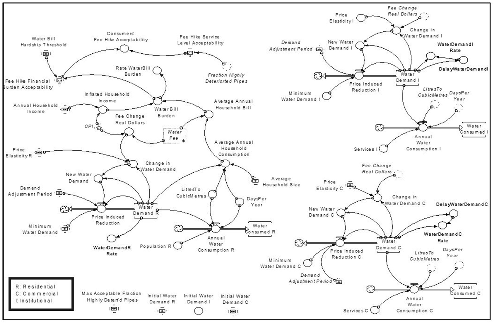
Figure 5. Socio-political sector of the advanced system dynamic model in Stella®.
Asset Management Strategy Implementation
The three decision-making layers developed for the asset management strategy of the water distribution network are validated using data from three water utilities in Southern Ontario, Canada, arbitrarily called X, Y, and Z.
Data and Parameters for Utilities X, Y, and Z
Strategic targets and policy levers controlling the strategic targets, as noted in Tables 2, 3, respectively, are made as identical as possible between each utility under the assumption that they will have similar preferences (due in part to their geographic proximity) for strategic targets, policy levers, sustainability, and life cycle. A capital reserve financing strategy is considered for all three utilities over a 100-year benchmarking period and is used to establish an annual capital reserve of 4% of the network replacement value.
The preferred network rehabilitation rate (Policy Lever 1) is set at 1.3% of the network per year to reflect desired utility practice and target rate recommended by The Canadian Infrastructure Report Card (2016). Policy Lever 2 allows water utilities to build up cash reserves of up to 4% of the replacement value of their network. Policy Lever 3 is set at 5%, indicating that the utility will allow up to 5% of its network pipes to be in the worst structural condition. If the 5% threshold is exceeded, a network rehabilitation rate higher than the preferred rate of 1.3% is required to eliminate deteriorated pipes in the network within the elimination period of 5 years (Policy Lever 4). Policy Lever 5 controls the peak fee hike rate and allows the water utilities to generate revenue to pay for capital and operational expenses and enable them to build up their target cash reserve. The optimal allowable water fee-hike rates (Policy Lever 5) for financially sustainable water distribution network management are 8.5% per annum for utility X, 9% per annum for utility Y, and 10.5% per annum for utility Z.
To simulate and run the advanced system dynamics model for the three water utilities, significant data have been collected on components/parameters of infrastructure, finance, and socio-political sectors. Demographic information of water utilities X, Y, and Z including population and water main length, are summarized in Table 4. Their networks are comprised of pipes made of Polyvinyl Chloride (PVC), Cast Iron (CI), Ductile Iron (DI), and Asbestos Cement (AC). Initially, 5.5, 8, and 8.5% of their respective network lengths are in the worst structural condition (i.e., more than 75 years old).
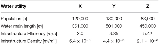
Table 4. Demographic information of water utilities.
The current water fees utilities charge their customers are CAD 1.55/m3, CAD 1.68/m3 and CAD 0.92/m3 for utilities X, Y, and Z, respectively. The current cost of water treatment is reported CAD 0.83/m3 for utilities X and Y and CAD 0.54/m3 for utility Z. Typical Average Daily Water Consumption in the local region are 280 l per capita per day (lpcd) for utilities X and Z and 322 lpcd for utility Y. The Minimum Water Demand for the three utilities is assumed to be 150 lpcd. Price Elasticity of Water Demand for the residential sector is assumed to be equal to −0.35, reported by Boland et al. (1984); Olmstead et al. (2007), and used by Rehan et al. (2011, 2014b, 2015); Ganjidoost et al. (2015b); Ganjidoost (2016).
The current unit cost for rehabilitating pipes 75–100 years old is reported CAD 600 per meter, and for pipes more than 100 years old, it is set at CAD 700 per meter for the three utilities. The unit operation and maintenance costs and leakage rate are calculated in a manner identical to Ganjidoost (2016). The 6.4% per annum inflation rate reported by Younis et al. (2016) for water main construction projects is used in this study to inflate the unit cost of pipe renewal ($/m), the unit cost of pipe maintenance ($/m/year), and the unit price of treated water ($/m3). The household income is inflated over the benchmarking period with the rate of 2.4% per annum reported by the Customer Price Index (CPI) of Canada (Statistics Canada, 2014).
Results and Discussions
This section presents the benchmarking results of the three interconnected decision-making layers for the asset management strategy of three water utilities over a 100-year benchmarking period, as illustrated in Figures 6–8.
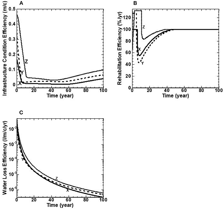
Figure 6. (A–C) Water infrastructure performance indicators over a 100-year benchmarking period for utilities X, Y, and Z.
Infrastructure Performance Indicators
This category measures the infrastructure performance of the water distribution network (see Table 1). The BPI of infrastructure efficiency and density for each utility are provided in Table 4. For this study, the water network length, population, and area serviced by the utility are assumed to be constant over the benchmarking period (all under the same assumptions). Therefore, the infrastructure efficiency and density with values noted in Table 4 are constant over the benchmarking period for the three utilities. However, the model can quantify development charges, network expansion and population growth/decline. These assumptions were made with respect to the three utilities inputs/insights to the model. The other three BPI's are presented for the three utilities to demonstrate (a) infrastructure condition efficiency (m/c), (b) rehabilitation efficiency (%/yr), and (c) water loss efficiency (l/m/c/yr). The performance indicators of this category are illustrated with water utilities X, Y, and Z in Figure 6.
The results of this category show that the three utilities achieve the stated strategic target of Min (infrastructure condition efficiency), with the controlling Policy Lever 1 (i.e., preferred rehab rate of 1.3% of the network per year), Policy Lever 3 (i.e., no more than 5% of pipes in the worst structural condition), and Policy Lever 4 (i.e., eliminating period of 5 years for pipes in the worst structural condition). In addition, the strategic target of Min (water loss) is achieved for the three utilities, as illustrated in Figure 6C. Therefore, the three water utilities sustainably maintain these targets over the life cycle of the infrastructure. It should be noted that all pipes are assumed to be replaced by PVC.
Figure 6A shows the BPI of infrastructure condition efficiency that measures an infrastructure system's efficiency in terms of a fraction of highly deteriorated pipes (+75 years) per capita (m/c). In general, the benchmarking results show the same trend for the three utilities. For water utility X, the infrastructure condition efficiency starts with a value of 0.17 m/c, decreases to 0.02 m/c at 6 years, then decreases linearly to the age of 60 years, followed by linear increases to the end of the benchmarking period to reach the value of 0.04 m/c (Figure 6A). For water utility Y, the infrastructure condition efficiency starts at a value of 0.34 m/c, declines to 0.02 m/c at 5 years, then increases linearly to the age of 42 years, followed by a decline to 58 years, and a continuous climb linearly to the end of the benchmarking period to reach a final value of 0.63 m/c (Figure 6A). For water utility Z, the infrastructure condition efficiency starts with a value of 0.47 m/c, decreases to 0.06 m/c at 10 years, continues to decline linearly to the age of 42 years, and then is followed by a continues increase linearly to the end of the benchmarking period to reach a final value of 0.1 m/c (Figure 6A).
Water utility Z has the highest fraction of highly deteriorated pipes (m/c) beyond 10 years. This is due to the allowable fee-hike rate for utility Z being set too low such that insufficient revenues exist to replace the fraction of highly deteriorated pipes at given times. However, all utilities eventually comply with Policy lever 4, such that no more than five percent of the network is in a deteriorated condition. This suggests that rehabilitating 1.3% of the network length per year (i.e., Policy Lever 1) appears to be achieved over the life-cycle of the infrastructure for all three water utilities.
Figure 6B shows the BPI of rehabilitation efficiency (%/yr). Water utility Z starts this benchmarking exercise with the oldest inventory of pipes and the highest fraction of deteriorated pipes (see Figure 6A). Consequently, it has the highest value of rehabilitation efficiency for the first 45 years of the benchmarking period, as shown in Figure 6B. Rehabilitation efficiency BPI measures the percentage of actual rehabilitation/replacement to the stated rehabilitation/replacement target. As this percentage approaches unity (i.e., 100%), the policy lever of rehabilitating/replacing 1.3% of the network length per year appears to be achieved over the life cycle of the infrastructure for all three water utilities.
For water utility X, the rehabilitation efficiency starts with a value of 100 percent, remains constant for 6 years, followed by a sudden decline to reach the minimum value of 52% at 10 years, and then is followed by a continuous increase to the age of 45 years to reach the value of 100 percent and remains constant to the end of benchmarking period (Figure 6B). For water utility Y, the rehabilitation efficiency starts with a value of 100%, climbs to 127% at 5 years, followed by a sudden decline to 42% at 7 years, and a continuous climb to 100 percent at 45 years and remains constant to the end of the benchmarking period (Figure 6B). For water utility Z, the rehabilitation efficiency starts with a value of 100 percent, followed by a continuous increase in the first 2.5 years to reach its maximum value of 132% at 2.5 years and remains constant to the age of 10 years, followed by a sudden decline to 85% at 15 years, and then followed by a continues climb to 100% at 45 years and remains constant to the end of the benchmarking period (Figure 6B).
Figure 6C depicts water loss efficiency BPI by measuring water loss per meter length of network per capita over the benchmarking period (l/m/c/yr). The water loss efficiency BPI starts with values of 0.036, 0.015 and 0.06 l/m/c/yr for water utilities X, Y and Z, respectively. This performance indicator declines for the three utilities implying that they all achieve the stated target of minimizing water loss over the benchmarking period. Utility Z has the highest water loss given as water loss divided by network length, population, and the benchmarking period (l/m/c/yr). This is a function of utility Z initially having the oldest inventory of pipes. In contrast, utility X has the lowest water losses, given its youngest inventory of pipes (Figure 6A).
Kleiner (1998) indicated that water loss from a pipe is a function of its structural condition. Utility Z starts this benchmarking exercise with the oldest inventory of pipes and the highest fraction of deteriorated pipes, whereas utility X starts with the youngest inventory of pipes and the lowest fraction of deteriorated pipes, as shown in Figure 6A. Therefore, more capital works are required for utility Z compare to the other two utilities, as shown in Figure 8D to reduce water loss and the associated expenditures, as shown in Figures 6C, 8B, respectively over the benchmarking period. Utilities X and Y show the same behavior as utility Z on water loss efficiency, as shown in Figure 6C.
Socio-Political Performance Indicators
This category measures the socio-political performance of three water utilities in terms of (a) fee hike ratio (%), (b) metered water efficiency (m3/m3), and (c) metered water loss ratio (m3/m3) (see Table 1). The results of this category show that the three utilities maintain the stated strategic targets of Min (Water Losses), as shown in Figures 7B,C.
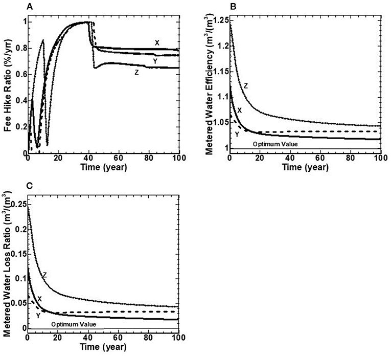
Figure 7. (A–C) Water socio-political indicators over a 100-year benchmarking period for utilities X, Y, and Z.
Figure 7A shows the fee-hike ratio BPI for the three water utilities. This performance indicator is measured as the percentage of current fee-hike to allowable fee-hike over the benchmarking period. The value of one indicates that the current fee-hike rate equals the allowable fee-hike ratio. The fee-hike ratio shows some oscillations in the first 30 years for all three water utilities (Figure 7A). The results show that this ratio hits the maximum value of unity at 30 years and remains constant between 4 and 5 years, followed by a sudden decline and continues to decrease linearly to the end of the benchmarking period to reach final values of 0.8, 0.75, and 0.65% for utilities X, Y, and Z, respectively (Figure 7A).
The BPI of metered water efficiency (m3/m3) as the ratio of supplied to metered water is illustrated in Figure 7B. The difference between supplied and metered water is water loss. The optimum value for this performance indicator is obtained with the value of unity, indicating no water loss exists in the water distribution network. The BPI of metered water efficiency starts with initial values of 1.12, 1.06, and1.25 for water utilities X, Y, and Z, respectively, followed by a decline to their minimum values of 1.02, 1.03, and 1.04, respectively, at the end of the benchmarking period. Figure 7B indicates that water utility Z has the highest metered water efficiency than the other two utilities due to its highest infrastructure condition efficiency, as shown in Figure 6A.
Figure 7C shows the metered water loss ratio BPI (m3/m3) as the ratio of water loss to metered water. It shows the initial values of 0.115, 0.07, and 0.24 for water utilities X, Y, and Z, respectively, followed by a decline to their minimum values of 0.02, 0.03, and 0.045, respectively at the end of the benchmarking period. A zero value represents the optimum value for the BPI of the metered water loss ratio, which means no water loss exists in the system or supplied water is equal to the metered water. Similar to the BPI of metered water efficiency, as depicted in Figure 7B, water utility Z has the highest water loss over the benchmarking period (Figure 7C).
Financial Performance Indicators
This category measures the financial performance of three water utilities in terms of (1) Water TotalEx Efficiency, (2) Water OpEx Efficiency, (3) Water CapEx Efficiency, (4) Non-RevenueEx Efficiency, (5) Water Debt Efficiency, (6) Liability-Asset Ratio, (7) OpEx Ratio and (8) CapEx Ratio (see Table 1). The water utility is not required to issue debt under the capital reserving scenario; thus, the BPI of water debt efficiency is over the benchmarking period for all three water utilities. The benchmarking results for the remaining seven financial performance indicators are illustrated in Figure 8. The results indicate that the three utilities meet the strategic targets of (1) Min (waterTotalExefficiency) by minimizing non-RevenueEx efficiency (Figure 8B), (2) Min (water loss); and (3) Min (liability).
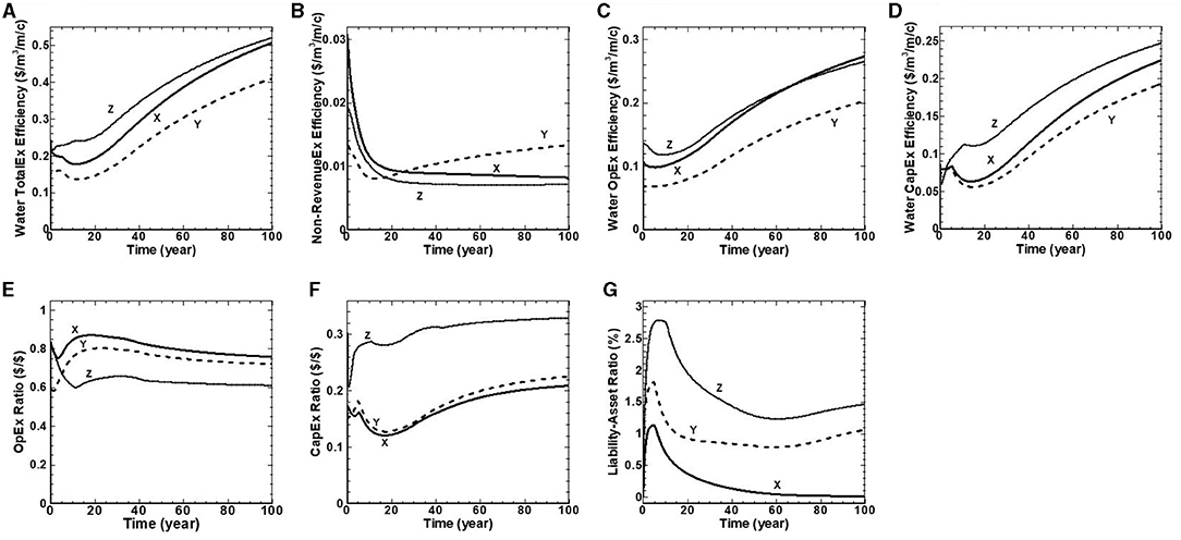
Figure 8. (A–G) Water financial performance indicators over a 100-year benchmarking period for utilities X, Y, and Z.
Figure 8A shows water TotalEx efficiency BPI for the three water utilities. In general, the results show a linear trend with some curvature. The water TotalEx efficiency BPI starts with a value of CAD 0.22/m3/m/c for water utilities X and Z, and CAD 0.16/m3/m/c for water utility Y, in the first 20 years followed by some oscillations, and continues to increase to the end of the benchmarking period to reach the value of CAD 0.5, CAD 0.41, and CAD 0.52/m3/m/c for utilities X, Y and Z, respectively (Figure 8A). Residents of utility Z spend more dollars per cubic meter of supplied water per meter of network length per capita compared to the other water utilities. In contrast, residents of utility Y spend the least dollars per cubic meter of supplied water per meter of network length per capita with the presumption that their water distribution system is the most efficient. This expense is essentially the ratio of total water distribution expenditures divided by supplied water ($/m3); and infrastructure efficiency (m/c). In summary, the three utilities ultimately achieve similar behavior over the entire benchmarking period, with the spread in their water TotalEx efficiency never separating by more than approximately CAD 0.11 m3/m/c. The spread persists due to the assumption of constant population and network length combined with the peak fee hikes rate that permits each water utility to have sufficient Revenue to meet expenses over the benchmarking period.
The non-RevenueEx efficiency BPI is illustrated in Figure 8B. This BPI is measured in terms of water loss expenditures per cubic meter of supplied water per meter of network length per capita. The non-RevenueEx efficiency starts with the initial values of $0.03, $0.01, and $0.02/m3/m/c for water utilities X, Y and Z, respectively. The results show the same declining trend for utilities X and Z to the end of the benchmarking period to reach their minimum values of CAD 0.008 and CAD 0.007/m3/m/c. For water utility Y, it starts with a value CAD 0.05/m3, declines for 10 years, and then is followed by a continuous increase to the end of benchmarking period to reach the value CAD 0.01 /m3/m/c (Figure 8B).
Figure 8C shows water OpEx efficiency BPI for the three water utilities. The results show the same trend for all three water utilities. The water OpEx efficiency BPI starts with initial values of CAD 0.11, CAD 0.07, and CAD 0.14/m3/m/c for water utilities X, Y and Z, respectively, in the first 20 years followed by some oscillations, and continues to increase to the end of the benchmarking period to reach the value of CAD 0.27, CAD 0.20, and CAD 0.26/m3/m/c for utilities X, Y, and Z, respectively (Figure 8C). All utilities achieve similar behavior over the entire benchmarking period, with the spread in their water OpEx efficiency never separating by more than approximately CAD 0.07 m3/m/c. In summary, the three utilities comply with the policy lever that no more than 5% of the network is in a deteriorated condition.
Figure 8D shows water CapEx efficiency BPI that is measured in terms of capital expenditures over the supplied water per meter of network length per capita. The water CapEx efficiency BPI starts with the initial values of CAD 0.08, CAD 0.06, and CAD 0.07/m3/m/c for water utilities X, Y, and Z, respectively. In general, the results show some oscillations in the first 20 years, followed by a linear increase to the end of the benchmarking period to reach the value of CAD 0.22, CAD 0.18, and CAD 0.25/m3/m/c for utilities X, Y, and Z, respectively (Figure 8D). All three utilities show the same behavior over the 100 years, with the spread in their water CapEx efficiency never separating by no more than CAD 0.07 m3/m/c, respectively. In summary, the three utilities comply with the policy lever that no more than 5% of the network is in a deteriorated condition.
Figure 8E shows OpEx ratio BPI for the three water utilities. The OpEx ratio BPI determines whether a water utility achieves its operational program targets by measuring the ratio of operational expenditures over the Revenue. Generally, the results show the same declining trend beyond 20 years. The OpEx ratio BPI starts with a value of 0.83, 0.69, and 0.80 for water utilities X, Y, and Z, respectively, and follows with some oscillations in the first 20 years, followed by a decline to the end of the benchmarking period to reach the values of 0.76, 0.72, and 0.61% for water utilities X, Y, and Z, respectively.
The CapEx ratio BPI for the three water utilities is illustrated in Figure 8F. The CapEx ratio BPI determines whether a water utility achieves its capital works targets by measuring the ratio of capital expenditures over the Revenue. In general, the results show a linear trend with some curvature. The CapEx ratio BPI starts with a value of 0.17, 0.12, and 0.20 for water utilities X, Y, and Z, respectively. In the first 15 years, it is followed by some oscillations and continues to increase to the end of the benchmarking period to reach the value of 0.21, 0.23, and 0.33% for utilities X, Y, and Z, respectively (Figure 8E). Water utility Z has the highest value of CapEx ratio BPI over the benchmarking period due to its oldest inventory of pipes and the highest infrastructure condition efficiency value (Figure 6A). Therefore, it requires spending more funds on capital works to comply with the policy lever that no more than 5% of the network in a deteriorated condition. Water utility X has the lowest value of CapEx ratio due to its lowest value of infrastructure condition efficiency (Figure 6A) beyond 5 years in the benchmarking period, as depicted in Figure 6C.
The BPI of liability-asset (L/A) ratio, as shown in Figure 8G is measured as a percentage of total liabilities relative to total assets for a water utility. The benchmarking result indicates that applying a capital reserving management strategy enables water utilities to reserve cash and have enough funds to accelerate capital works projects with no or minimal liability over the benchmarking period. The L/A BPI starts with the initial value of 0% for all three water utilities indicating no liability at time zero, followed by an increase to reach its maximum value of 1.1, 1.8, and 2.8% for utilities X, Y, and Z, respectively, and declines to the end of the benchmarking period to reach the value of 0, 1.1, and 1.5% for utilities X, Y, and Z, respectively, at the end of benchmarking period.
Effect of Desired Cash Reserve on Infrastructure and Financial BPI's
The three water utilities' performance over the 100-year benchmarking period discussed in the previous section involved only a 4% desired cash reserve. Moreover, each water utility had a common set of allowable fee-hike with a 1.3% preferred network rehabilitation rate for the three utilities. To gain further insights regarding the impact of desired cash reserve on infrastructure and financial performance indicators, it is instructive to explore network management strategies over a broader range of two policy levers: (1) allowable fee-hike rate, and (2) network rehabilitation rate, as noted in section Data and Parameters for Utilities X, Y, and Z. This is accomplished by creating three scenario sets corresponding to desired cash reserve values of 1, 2.5, and 4%. Within each scenario set, the allowable fee-hike rate is varied over a range of 0 to 12% per annum, and the preferred network rehabilitation rate is varied over a range of 0–3% per annum. It is assumed that an allowable fee-hike rate in excess of 12% per annum is not a politically feasible strategy for the water utility to sustain over the long run. Similarly, a capital-works plan rehabilitating in excess of 3% of the network per year is assumed not feasible due to the availability of physical and financial resources. Policy levers for the three scenario sets are provided in Table 5. The effect of the desired cash reserve is presented on two selected BPI's that represent the infrastructure and financial performance of water utilities. The BPI of infrastructure condition efficiency (m/c) is selected for infrastructure performance, and the BPI of water TotalEx efficiency ($/m3/m/c) is selected for the financial performance of the utility over the benchmarking period.
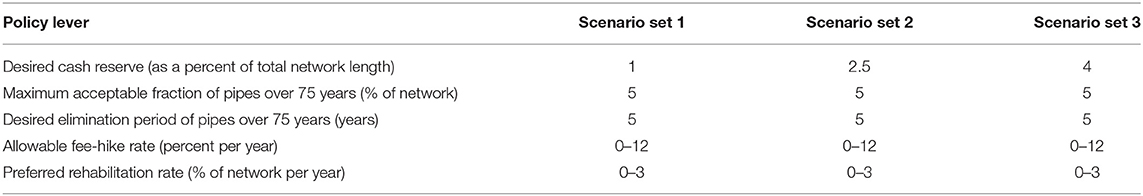
Table 5. Policy levers for three scenario sets.
Figures 9A–C present the contours of maximum BPI of infrastructure condition efficiency that is the length of pipes over 75 years per capita (m/c) for scenarios 1, 2, and 3 with 1, 2.5, and 4% desired cash reserve, respectively. These contours are the mean BPI values arising from the simulations (3,969 runs) for the three utilities. For comparative purposes, water utilities X, Y, and Z with the unique set of allowable fee hike and a 1.3% preferred network rehabilitation, as discussed in the previous section, are illustrated as white dots on Figures 9A–C, respectively. Figures 8E,F, 9D show contours of the water TotalEx efficiency, as measured in terms of total water distribution expenditures divided by supplied water per length of water network per capita ($/m3/m/c), at 100 years for scenarios with 1, 2.5, and 4% desired cash reserve, respectively. These contours are also the mean BPI values arising from the simulations (3,969 runs) for the three utilities. Once again, for comparative purposes, water utilities X, Y, and Z are depicted as white dots on Figures 8E,F, 9D, respectively.
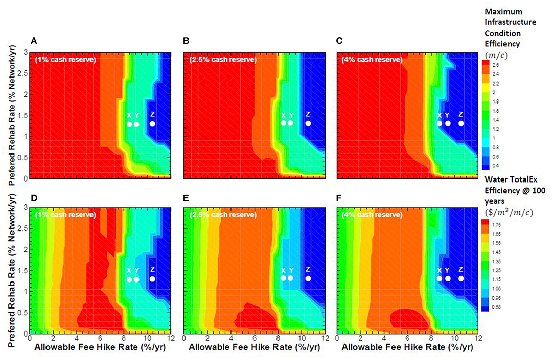
Figure 9. (A–F) Impact of allowable fee-hike and preferred rehabilitation rates on infrastructure condition efficiency and water TotalEx efficiency.
Figures 9A–C indicate that the value of infrastructure condition efficiency (m/c) decreases as the allowable fee-hike rate increases over the benchmarking period. The least (m/c) region is shown with a blue contour for desired cash reserve of 1, 2.5, and 4%. From a socio-political and administrative perspective, it is desirable for the water utility to operate on the boundary of the blue contour. The results of Figures 9A,B show that the desired cash reserve of 1 and 2.5% do not provide sufficient funds for the original scenarios of water utilities X and Y (section Data and Parameters for Utilities X, Y, and Z), as depicted with white dots on Figures 9A,B, respectively to be in or near the blue region. The desired cash reserve of 4% provides sufficient funds for utilities X and Y to move into the blue region, as illustrated in Figure 9C. For the original scenario of water utility Z (section Data and Parameters for Utilities X, Y, and Z), as shown with dots on Figures 9A–C, the value of infrastructure condition efficiency BPI shows the same behavior with desired cash reserve from 1 to 4% and remains in the blue region.
Figures 9D–F indicate that the water TotalEx efficiency, as a financial BPI, has a similar shape to the infrastructure condition efficiency and decreases as the allowable fee-hike rate increases over the benchmarking period. The least ($/m3/m/c) region is shown with blue contour for desired cash reserve of 1, 2.5, and 4%. The results of Figures 9D,E show that the desired cash reserve of 1 and 2.5% do not provide enough funds for the original scenarios of water utilities X and Y (section Data and Parameters for Utilities X, Y, and Z), as depicted with white dots on Figures 9D,E, respectively, to be in or near the blue region. The desired cash reserve of 4% provides utilities X and Y with sufficient funds to move into the blue region, as illustrated in Figure 9F. For the original scenario of water utility Z (section Data and Parameters for Utilities X, Y, and Z), as shown with dots on Figures 9D–F, the value of water TotalEx efficiency shows similar behavior with desired cash reserve from 1 to 4% and remains in the blue region.
Note that these contours are stable in the sense that the three utilities are used to create them. Hence, more data from additional utilities could be used to depict an optimal global solution for all utilities to conform to.
The most important observation is that contours representing the “optimal” combination of allowable fee-hike rate and preferred rehabilitation rate in terms of minimizing either the infrastructure condition efficiency, as infrastructure BPI or the water TotalEx efficiency, as financial BPI have the same shape. In other words, both indicators can be optimized simultaneously by adjusting the two policy levers: (1) allowable fee-hike rate, and (2) preferred network rehabilitation rate for a given cash reserve. In summary, water utilities should select the optimal combinations of allowable fee hike and preferred rehabilitation rates that are on the boundary of the blue-contour region which enables them to sustainably achieve the stated targets over the life-cycle of water mains.
Conclusions
This study demonstrates a unified implementation framework for the asset management strategy of water utilities to meet sustainable infrastructure, socio-political, and financial targets over the life cycle of the infrastructure. The advanced system dynamics model enables three customized models for each independent utility to represent their infrastructure, financial and socio-political characteristics. The advanced system dynamics model (i.e., Function layer) enables water utilities to plan future actions required to meet stakeholders' objectives. Also, the water utility can benchmark and compare success at achieving their strategic targets established in the Visions and Values layer across utilities regardless of the utility size. The application of the entire BPI's demonstrates the complexity of the water distribution system and allows a better understanding of the total system responses.
Based on this study, the following conclusions can be drawn:
1. An advanced system dynamics model is developed to forecast the future behavior of water distribution networks.
2. The output of the advanced system dynamics model is then used to demonstrate the first known application of the entire benchmarking performance indicators for water distribution networks developed by Ganjidoost et al. (2018).
3. An implementation framework for asset management strategy of water distribution networks is developed comprised of three decision-making layers: (1) Visions and Values, (2) Function, and (3) Performance.
4. Benchmarking results indicate that all three water utilities can sustainably meet the strategic targets established in the Visions and Values layer of the asset management strategy over the benchmarking period.
5. The “optimal” combinations of allowable fee-hike and rehabilitation rates along with a capital reserving management strategy (i.e., cash reserve) will allow water utilities to have sufficient funds to meet their strategic targets.
6. The performance modeling and simulation approach presented in this study represents a powerful tool for other utilities to develop optimal strategic and operational plans for their networks and thus better service to their stakeholders.
Future works are recommended to further refine and expand the scope of the presented framework for the asset management strategy of water distribution networks. The study presented in this paper was limited to the water distribution pipelines. Further works can be done to include other components of the water distribution network such as valves, pumps, and service connections, or use the underlying conceptual ideas of this framework to create specific and integrated frameworks for the asset management strategy of sewer, storm, and treatment plants.
Water utilities, consultants, researchers, and any entity interested in this subject matter are also encouraged to use the the BPI's presented in this study as a baseline/guideline to develop their own normalized and time-integrated BPI's such as fire flow availability, or pump energy efficiency to demonstrate their long-term sustainability over the life cycle of assets.
Due to the lack of data obtained from the three case utilities, the degradation rate was assumed to exponentially increases as pipes aging. This is only assumed to demonstrate the application of the model under identical assumptions for all three case utilities to benchmark their behavior over the simulation period. Further research can be done to support the advanced system dynamics model of this study with the actual structural health of water mains. The outputs of this study provide a good indication for the utility stakeholders of the need to conduct and collect condition assessment data of theirs water mains.
For this study, the water network length and population serviced by the utility were assumed to be constant over the benchmarking period with respect to the three utilities inputs/insights to the model. From the utility's financial perspective, population growth doesn't necessarily mean more fund balance because at the same time water demands increase and the water utility requires supplying more water. With more new vertical developments, many network expansions cannot be expected because the new needs could be satisfied with a pipe replacement to carry more flow to the new customers. The system dynamics model and framework presented in this study can be used by any utilities (regionally, nationally, or globally) with the combinations of different scenarios to provide a trend over the simulation period. However, future works can be done to explore the impacts of network expansion and population growth/decline on the utility's infrastructure, socio-political, and financial targets.
Data Availability Statement
The original contributions presented in the study are included in the article/supplementary material, further inquiries can be directed to the corresponding author/s.
Author Contributions
AG: main researcher and developer of this paper. MK, AU, and CH: research advisors and co-investigators of the research. All authors contributed to the article and approved the submitted version.
Conflict of Interest
AG was employed by the company Xylem Inc.
The remaining authors declare that the research was conducted in the absence of any commercial or financial relationships that could be construed as a potential conflict of interest.
Publisher's Note
All claims expressed in this article are solely those of the authors and do not necessarily represent those of their affiliated organizations, or those of the publisher, the editors and the reviewers. Any product that may be evaluated in this article, or claim that may be made by its manufacturer, is not guaranteed or endorsed by the publisher.
Acknowledgments
The authors gratefully acknowledge the financial support provided by the Natural Science and Engineering Council of Canada, the University of Waterloo, and the Center for Advancement of Trenchless Technologies located at the University of Waterloo. And also acknowledge the City of Waterloo, the City of Niagara Falls, and the City of Cambridge for their financial support, provision of data, and sharing of valuable insights on water utility management.
References
AWWA (2010). Water Transmission and Distribution. Principles and Practices of Water Supply Operations Series. Denver, CO: AWWA.
Boland, J. J., Dziegielewski, B., Baumann, D. D., and Optiz, E. M. (1984). Influence of Price and Rate Structures on Municipal and Industrial Water Use. Carbondale, IL: Planning and Management Consultants Ltd.
British Standard Institution. (2014). (BS ISO 55000:2014): Asset Management-Overview, Principles and Terminology, 1st Edn. BSI Standards.
Ganjidoost, A. (2016). Performance Modeling and Simulation for Water Distribution and Wastewater Collection Networks. UWSpace.
Ganjidoost, A., Haas, C., Knight, M., and Unger, A. (2015b). “A system dynamics model for integrated water infrastructure asset management,” in The Proceedings of the 33rd International Conference of the System Dynamics Society (Cambridge).
Ganjidoost, A., Knight, M. A., Unger, A. J. A., and Haas, C. T. (2018). Benchmark performance indicators for utility water and wastewater pipelines infrastructure. J. Water Resour. Plann. Manag. 144:04018003.G doi: 10.1061/(ASCE)WR.1943-5452.0000890
Ganjidoost, A., Younis, R., and Knight, M. (2015a). “Water mains degradation analysis using log-linear models,” in Pipelines (Maryland: ASCE), 1181–1194.
Kleiner, Y. (1998). Water Distribution Network Rehabilitation: Selection and Scheduling of Pipe Rehabilitation Alternatives. University of Toronto.
Lloyd, C., (ed.). (2010). Asset Management Whole-Life Management of Physical Assets. London: Thomas Telford Ltd.
Olmstead, S. M., Hanemann, W. M., and Stavins, R. N. (2007). Water demand under alternative price structures. J. Environ. Econ. Manag. 54, 181–198. doi: 10.3386/w13573
Rehan, R., Knight, M. A., Haas, C. T., and Unger, A. J. A. (2011). Application of system dynamics for developing financially self-sustaining management policies for water and wastewater systems. Water Res. 45, 4737–4750. doi: 10.1016/j.watres.2011.06.001
Rehan, R., Knight, M. A., Unger, A. J. A., and Haas, C. T. (2013). Development of a system dynamics model for financially sustainable management of municipal watermain networks. Water Res. 47, 7184–7205. doi: 10.1016/j.watres.2013.09.061
Rehan, R., Knight, M. A., Unger, A. J. A., and Haas, C. T. (2014a). Financially sustainable management strategies for urban wastewater collection infrastructure-development of a system dynamics model. Tunnell. Underground Space Technol. 39, 116–129. doi: 10.1016/j.tust.2012.12.003
Rehan, R., Unger, A. J. A., Knight, M. A., and Haas, C. T. (2014b). Financially sustainable management strategies for urban wastewater collection infrastructure-Implementation of a system dynamics model. Tunnell. Underground Space Technol. 39, 102–115. doi: 10.1016/j.tust.2012.12.004
Rehan, R., Unger, A. J. A., Knight, M. A., and Haas, C. T. (2015). Strategic water utility management and financial planning using a new system dynamics tool. J. AWWA 107:E22–E36. doi: 10.5942/jawwa.2015.107.0006
Statistics Canada (2014). Available online at: http://www.statcan.gc.ca/start-debut-eng.html (cited April 22, 2014).
Keywords: performance modeling, water distribution, benchmarking, asset management, strategic planning
Citation: Ganjidoost A, Knight MA, Unger AJA and Haas CT (2021) Performance Modeling and Simulation for Water Distribution Networks. Front. Water 3:718215. doi: 10.3389/frwa.2021.718215
Received: 31 May 2021; Accepted: 27 September 2021;
Published: 01 November 2021.
Edited by:
Elnaz Peyghaleh, Independent Researcher, Columbia, United StatesReviewed by:
Harshit Shukla, Texas A&M University, United StatesSomayeh Mohammadi, University of Maryland, United States
Copyright © 2021 Ganjidoost, Knight, Unger and Haas. This is an open-access article distributed under the terms of the Creative Commons Attribution License (CC BY). The use, distribution or reproduction in other forums is permitted, provided the original author(s) and the copyright owner(s) are credited and that the original publication in this journal is cited, in accordance with accepted academic practice. No use, distribution or reproduction is permitted which does not comply with these terms.
*Correspondence: Amin Ganjidoost, YW1pbi5nYW5qaWRvb3N0QHh5bGVtLmNvbQ==; YWdhbmppZG9AdXdhdGVybG9vLmNh